Ellipsoidal Oscillations Induced by Substellar Companions:
A Prospect for the Kepler Mission

Abstract

Hundreds of substellar companions to solar-type stars will be discovered with the Kepler satellite. Kepler’s extreme photometric precision gives access to low-amplitude stellar variability contributed by a variety of physical processes. We discuss in detail the periodic flux modulations arising from the tidal force on the star due to a substellar companion. An analytic expression for the variability is derived in the equilibrium-tide approximation. We demonstrate analytically and through numerical solutions of the linear, nonadiabatic stellar oscillation equations that the equilibrium-tide formula works extremely well for stars of mass $<$$1.4\,M_{\odot}$ with thick surface convection zones. More massive stars with largely radiative envelopes do not conform to the equilibrium-tide approximation and can exhibit flux variations $\gtrsim$10 times larger than naive estimates. Over the full range of stellar masses considered, we treat the oscillatory response of the convection zone by adapting a prescription that A. J. Brickhill developed for pulsating white dwarfs. Compared to other sources of periodic variability, the ellipsoidal lightcurve has a distinct dependence on time and system parameters. We suggest that ellipsoidal oscillations induced by giant planets may be detectable from as many as $\sim$100 of the $10^{5}$ Kepler target stars. For the subset of these stars that show transits and have radial-velocity measurements, all system parameters are well constrained, and measurement of ellipsoidal variation provides a consistency check, as well as a test of the theory of forced stellar oscillations in a challenging regime.

1. INTRODUCTION

The upcoming Kepler satellite will continuously monitor $\sim$$10^{5}$ main-sequence stars of mass $\simeq$0.5–$1.5\,M_{\odot}$ over 4–6 years with fractional photometric precisions of $\sim$$10^{-5}$. Such high sensitivity, which is unattainable from the ground, will allow for the robust detection of Earth-size planets that transit their host stars, and the measurement of asteroseismic oscillations as a probe of stellar structure (e.g., Borucki et al., 2004; Basri et al., 2005). These missions will also discover hundreds of “hot Jupiters” with orbital periods of $<$10 days, revealed by their transits or reflected starlight (e.g., Jenkins & Doyle, 2003). Continuous observations of these systems are likely to show a myriad of novel physical effects, including Doppler flux variability of the host stars (Loeb & Gaudi, 2003), photometric dips due to moons or rings around the planets (Sartoretti & Schneider, 1999; Brown et al., 2001), and the impact of additional perturbing planets on transit timing (Miralda-Escudé, 2002; Agol et al., 2005; Holman & Murray, 2005). The same ideas apply if the companion is a more massive brown dwarf, but these are rarely found in close orbits around solar-type stars (e.g., Grether & Lineweaver, 2006).

Here we scrutinize another mechanism for generating periodic variability of a star closely orbited by a giant planet or brown dwarf. A star subject to the tidal gravity of a binary companion has a nonspherical shape and surface-brightness distribution. In the simplest approximation, the stellar surface is a prolate ellipsoid with its long axis on the line connecting the two objects. As the tidal bulge tracks the orbital motion, differing amounts of light reach the observer. For a solar-type star orbited by a perturbing companion of mass $M_{p}$ with period $P_{\rm orb}$, the expected fractional amplitude of this ellipsoidal variability is $\sim$$10^{-2}(M_{p}/M_{\odot})(1\,{\rm day}/P_{\rm orb})^{2}$. This effect has a long history in the study of eclipsing binary stars (see the review by Wilson, 1994), but was mentioned only recently in the exoplanet context.

Udalski et al. (2002), Drake (2003), and Sirko & Paczyński (2003) noted that if ellipsoidal light variations are detected from the ground, where the fractional photometric precision is $\gtrsim$$10^{-3}$, then the perturber must be fairly massive (e.g., $\gtrsim$$0.1\,M_{\odot}$). They offered this idea as a test to distinguish between planetary transits and eclipses by low-mass stars. The superior sensitivity of Kepler offers the possibility of measuring ellipsoidal variability induced by giant planets ($M_{p}\sim 10^{-3}$–$10^{-2}\,M_{\odot}$) with orbital periods of $\lesssim$10 days.

Loeb & Gaudi (2003) compare the ellipsoidal variability induced by a planetary companion to flux modulations arising from reflected starlight and the Doppler effect. The three amplitudes are similar when the companion has an orbital period of $\lesssim$3 days and an optical albedo of $\lesssim$0.1. In a sufficiently long observation it should be possible to separately extract each of the signals, since their Fourier decompositions are distinct. Precise physical modeling of the ellipsoidal lightcurve could provide an independent constraint on the mass of the companion, as well as important clues regarding stellar tidal interactions.

Ellipsoidal variability is typically modeled under the assumption that the distorted star maintains hydrostatic balance and precisely fills a level surface of an appropriate potential (e.g., the Roche potential). The measured flux is then just an integral of the intensity over the visible stellar surface, where the intensity includes the effects of limb darkening and gravity darkening (e.g., Kopal, 1942). This approach is strictly valid only when the orbit is circular and the star rotates at the orbital frequency, so that a stationary configuration exists in the coorbital frame. These conditions may not be satisfied when the companion has a low mass or long period, because of the weak tidal interaction. In fact, a state of tidal equilibrium may not be attainable in the case of a planetary companion (e.g., Rasio et al., 1996). Equilibrium models of ellipsoidal lightcurves do have a realm of validity for noncircular orbits and asynchronously rototating stars, and have been applied successfully to somewhat eccentric binaries (e.g., Soszynski et al., 2004). However, by construction, such models ignore fluid inertia and the possibility exciting normal modes of oscillation, effects that may be of critical importance in a wide range of observationally relevant circumstances. Here we apply the machinery of linear stellar oscillation theory to the weak tidal forcing of stars by substellar companions. Conceptually, our investigation bridges Kepler’s planetary and astroseismology programs.

Section 2 describes the geometry of the problem, provides quantitative measures for the strength of the tidal interaction, discusses our simplifying assumptions, and presents the mathematical framework for calculating ellipsoidal variability. In § 3, we consider the equilibrium-tide approximation and derive an analytic expression for the ellipsoidal lightcurve. A brief review of von Zeipel’s theorem and its limitations is given in § 4. Tidally forced, nonadiabatic stellar oscillations are addressed in § 5, where we argue for a simple treatment of perturbed surface convection zones, use this prescription to calculate the ellipsoidal variability of deeply convective stars, estimate analytically the surface flux perturbation in mainly radiative stars, and show select numerical results. Our main conclusions are summarized in § 6. We conclude in § 7 with remarks on the measurement of ellipsoidal oscillations in the presence of other sources of periodic variability.

2. PRELIMINARIES

Consider a star of mass $M$ and radius $R$ is orbited by a substellar companion of mass $M_{p}$ and radius $R_{p}$. We work in spherical coordinates $(r,\theta,\phi)$ with the origin at the star’s center and the pole direction ($\theta=0$) parallel to the orbital angular momentum vector. The orbit is then described by $(d,\pi/2,\phi_{p})$, where $d$ and $\phi_{p}$ are, respectively, the time-dependent orbital separation and true anomaly; $\phi_{p}=0$ marks the phase of periastron. We assume that the orbit is strictly Keplerian with fixed semimajor axis $a$ and eccentricity $e$, such that $d=a(1-e^{2})/(1+e\cos\phi_{p})$. The direction to the observer from the center of the star is $(\theta_{o},\phi_{o})$, so that the conventional orbital inclination is $I=\pi-\theta_{o}$.

We imagine that the gravity of the companion raises nearly symmetrical tidal bulges on opposite sides of the star that rotate at the orbital frequency. A rough measure of both the height of the tides relative to the unperturbed stellar radius and the fractional amplitude of the ellipsoidal variability is given by the ratio of the tidal acceleration to the star’s surface gravity:

$$\varepsilon\equiv\frac{M_{p}}{M}\left(\frac{R}{a}\right)^{3}\sim 10^{-5}\,\frac{M_{p}}{M_{J}}\frac{M_{\odot}}{M}\left(\frac{P_{*}}{2.8\ {\rm hr}}\frac{1\ {\rm day}}{P_{\rm orb}}\right)^{2}~{},$$ (1)

where $M_{J}\simeq 10^{-3}\,M_{\odot}$ is the mass of Jupiter, $P_{*}=2\pi(R^{3}/GM)^{1/2}=2.8\,[(R/R_{\odot})^{3}(M_{\odot}/M)]^{1/2}\,{\rm hr}$ is the dynamical time of the star. For main-sequence stars with $R/R_{\odot}\simeq M/M_{\odot}$, we see that $\varepsilon\propto M_{p}MP_{\rm orb}^{-2}$. The maximum value of $\varepsilon$ is attained when the companion fills its Roche lobe at an orbital separation of $a\simeq 2R_{p}(M/M_{p})^{1/3}$, which gives

$$\varepsilon_{\rm max} \simeq \left(\frac{M_{p}}{M}\right)^{2}\left(\frac{R}{2R_{p}}\right)^{3}$$ (2)

$$\simeq 10^{-4}\,\left(\frac{M_{p}}{M_{J}}\right)^{2}\frac{M}{M_{\odot}}\left(\frac{0.1\,R_{\odot}}{R_{p}}\right)^{3}~{},$$

where we have applied a fixed value of $R_{p}=0.1\,R_{\odot}$, appropriate for both giant planets and old brown dwarfs. Note that $\varepsilon_{\rm max}\sim 1$ for massive brown dwarfs ($M_{p}/M_{J}\sim 80$). Hereafter, we consider only cases with $\varepsilon\ll 1$.

For orbital periods as short as $\simeq$1 day, tidal torques on the star from a planetary companion are rather ineffective at altering the stellar rotation rate (e.g., Rasio et al., 1996). Therefore, as already mentioned in § 1, we should not generally expect the star to rotate synchronously with the orbit, and so there is no frame in which the star appears static. This holds when the orbit is circular, and is obviously true when the there is a finite eccentricity. In fact, $\simeq$30% of the known exoplanets with $P_{\rm orb}<10$ days have eccentricities of $>$0.1. Small variable distortions of the star from its equilibrium state, due to a combination of asynchronous rotation and orbital eccentricity, should be viewed as waves excited by the tidal force of the companion. Our task is to study such tidally forced stellar oscillations in the linear domain in order to understand the corresponding lightcurves.

In order to greatly simplify the mathematical description of the stellar oscillations, we assume that the star is nonrotating in the inertial frame. When the stellar rotation frequency is nonzero, but much smaller than the tidal forcing frequency, the effect of rotation is to introduce fine structure into the oscillation frequency spectrum, and cause the oscillation eigenfunctions to be slightly modified as a result of the Coriolis force (for a discussion, see Unno et al., 1989). Tidal pumping of a slowly rotating star by an orbiting companion has a dominant period of $P_{\rm orb}/2$—a few days in the cases of interest. By contrast, single solar-type stars with ages $>$1 Gyr tend to have rotation periods of $>$10 days (e.g., Skumanich, 1972; Pace & Pasquini, 2004); the Sun has an equatorial rotation period of $\simeq$25 days. Slowly rotating stars with masses of $\simeq$$1\,M_{\odot}$ are prime targets for Kepler, since they exhibit low intrinsic variability. Based on this selection effect, and the inability of tidal torques to spin up the star, our assumption of vanishing stellar rotation seems generally justified.

The general framework for calculating the measurable flux modulations associated with ellipsoidal stellar oscillations is as follows. We consider small perturbations to a spherical, nonrotating background stellar model, such that fluid elements at equilibrium position $\mathbf{x}$ are displaced in a Lagrangian fashion to position $\mathbf{x}+{\mbox{\boldmath$\xi$}}$. Variations in the measured flux from an oscillating star arise from two physically distinct contributions (e.g., Dziembowski, 1977): (1) changes in the shape of the star due to radial fluid displacements $\xi_{r}={\mbox{\boldmath$\xi$}}\cdot\mathbf{e}_{r}$, where $\mathbf{e}_{r}$ is the radial unit vector, and (2) hot and cold spots generated by local Lagrangian perturbations $\Delta F$ to the heat flux. Our main task in §§ 3 and 5 is to compute $\xi_{r}$ and $\Delta F$ according to the relevant physics.

Given the dependences of $\xi_{r}$ and $\Delta F$ on $(r,\theta,\phi)$, it is straightforward to compute the time varying component of the measured flux. The flux received from a star at distance $D$ is (e.g., Robinson et al., 1982)

$$\mathscr{F} = \frac{1}{D^{2}}\int dS\ \mathbf{n}\cdot\mathbf{n}_{o}\ F\ h(\mathbf{n}\cdot\mathbf{n}_{o})$$ (3)

where $dS$ is an area element at the stellar photosphere, $F$ is the net flux of radiation out of the surface element, $h$ is the limb-darkening function, $\mathbf{n}$ and $\mathbf{n}_{o}$ are unit vectors normal to the surface and toward the observer, respectively, and the integration is over the visible stellar disk. Vertical displacement at the surface yields changes in $\mathscr{F}$ through changes in surface area and $\mathbf{n}\cdot\mathbf{n}_{o}$. Following Dziembowski (1977), we expand $\xi_{r}$ and $\Delta F$ in spherical harmonics,

$$\xi_{r}(r,\theta,\phi,t) = \sum_{\ell=0}^{\infty}\sum_{m=-\ell}^{\ell}\xi_{r,\ell m}(r,t)Y_{\ell m}(\theta,\phi)~{},$$ (4)

$$\Delta F(r,\theta,\phi,t) = \sum_{\ell=0}^{\infty}\sum_{m=-\ell}^{\ell}\Delta F_{\ell m}(r,t)Y_{\ell m}(\theta,\phi)~{},$$ (5)

and carry out the appropriate linear expansions to obtain the fractional variability

$$\frac{\delta\mathscr{F}}{\mathscr{F}}=\sum_{\ell=0}^{\infty}\left[(2b_{\ell}-c_{\ell})\frac{\xi_{r,\ell}^{o}}{R}+b_{\ell}\frac{\Delta F_{\ell}^{o}}{F}\right]~{}.$$ (6)

Here $\xi_{r,\ell}^{o}$ and $\Delta F_{\ell}^{o}$ are components evaluated at the surface ($r=R$) and in the direction of the observer:

$$\frac{\xi_{r,\ell}^{o}}{R} = \sum_{m=-\ell}^{\ell}\frac{\xi_{r,\ell m}(R,t)}{R}Y_{\ell m}(\theta_{o},\phi_{o})~{},$$ (7)

$$\frac{\Delta F_{\ell}^{o}}{F} = \sum_{m=-\ell}^{\ell}\frac{\Delta F_{\ell m}(R,t)}{F}Y_{\ell m}(\theta_{o},\phi_{o})~{}.$$ (8)

The terms $b_{\ell}$ and $c_{\ell}$ are given by

$$b_{\ell}=\int_{0}^{1}d\mu\mu\,P_{\ell}\,h~{},~{}~{}c_{\ell}=\int_{0}^{1}d\mu(1-\mu^{2})\frac{dP_{\ell}}{d\mu}\left(h+\mu\frac{dh}{d\mu}\right)\ ,$$ (9)

where $\mu=\mathbf{n}\cdot\mathbf{n}_{o}$, the $P_{\ell}(\mu)$ are ordinary Legendre polynomials, and $h(\mu)$ is normalized such that $\int_{0}^{1}d\mu\mu\,h=1$. The linear limb-darkening function is

$$h(\mu)=\frac{6}{(3-\gamma)}\big{[}1-\gamma(1-\mu)\big{]}~{};$$ (10)

more general nonlinear functions of $\mu$ (e.g., Claret, 2000) will not be considered here. The classical Eddington limb-darkening function is $h=1+3\mu/2$ ($\gamma=3/5$; e.g., Mihalas, 1970). Table 1 shows shows functional forms and particular values of $b_{\ell}$ and $c_{\ell}$ for $\ell=2$ and 3.

3. EQUILIBRIUM TIDE

Vertical displacement of the stellar surface is often accurately modeled by assuming that the tidally perturbed fluid remains in hydrostatic balance. The cause and magnitude of the surface flux perturbation is a more complicated affair. In this section, we apply a simple parameterization of the flux perturbation and obtain a complete set of formulae for computing the ellipsoidal lightcurve. Subsequent sections provide more detailed calculations. In particular, we show in § 5.2 that stars with deep convective envelopes (the majority of Kepler targets) have surface flux variations that conform to the equilibrium-tide approximation.

Table 1Limb Darkening Parameters

		$b_{\ell}$			$c_{\ell}$
$\ell$		General $\gamma$	$\gamma=3/5$		General $\gamma$	$\gamma=3/5$
2		$(1+\gamma)/[20(3-\gamma)]$	13/40		$3(1+3\gamma)[10(3-\gamma)]$	39/20
3		$\gamma/[4(3-\gamma)]$	1/16		$3\gamma/(3-\gamma)$	3/4

When the tidal forces on the stellar fluid change sufficiently slowly, the star can stay very nearly in hydrostatic equilibrium. If the net acceleration required to balance the pressure gradient is derivable from a potential, then equilibrium implies that a fluid element remains on an equipotential surface. Since we neglect stellar rotation, there is no centrifugal force, and the total potential is the sum of the gravitational potential $\varphi$ from the spherical background stellar model and the perturbing tidal potential $U\sim\varepsilon\varphi\ll\varphi$. For our analytic work, we neglect the modification of $\varphi$ due to the tide. In general, the Eulerian variation $\delta\varphi$ should be added to $U$, as we do in our numerical models (see § 5.4 and the Appendix); we find that $|\delta\varphi|/|U|\sim 10^{-2}$.

In the absence of tidal forces, a given fluid element sits at equilibrium position $\mathbf{x}$ with total potential $\varphi(\mathbf{x})$. Gentle inclusion of the tidal potential causes the fluid element to move to position $\mathbf{x}+{\mbox{\boldmath$\xi$}}$ while preserving the value of the total potential. This is expressed mathematically by

$$\varphi({\mathbf{x}}) = \varphi(\mathbf{x}+{\mbox{\boldmath$\xi$}})+U(\mathbf{x}+{\mbox{\boldmath$\xi$}},t)$$ (11)

$$= \varphi(\mathbf{x})+{\mbox{\boldmath$\xi$}}\cdot\boldsymbol{\nabla}\varphi+U(\mathbf{x},t)+{\cal O}(\xi^{2},\xi U)~{}.$$

We see that ${\mbox{\boldmath$\xi$}}\cdot\boldsymbol{\nabla}\varphi=\xi_{r}g$, where $g=GM_{r}/r^{2}$ is the background gravitational acceleration at mass coordinate $M_{r}$. To first order, the radial displacement of the equilibrium tide is (see also Goldreich & Nicholson, 1989)

$$\xi_{r}(\mathbf{x},t) \simeq -U(\mathbf{x},t)/g~{},$$ (12)

which tells us the geometry of the star as a function of time.

The tidal potential within the star can be expanded as

$$U(r,\theta,\phi,t)=-\frac{GM_{p}}{d}\sum_{\ell=2}^{\infty}\left(\frac{r}{d}\right)^{\ell}P_{\ell}(\cos\psi)~{},$$ (13)

where $\cos\psi=\sin\theta\cos(\phi_{p}-\phi)$. There is no $\ell=1$ term, since this would give the acceleration of the star’s center of mass, which is already incorporated into the orbital dynamics. The angular expansion of $\xi_{r}$ follows immediately from eq. (12):

$$\frac{\xi_{r}(r,\theta,\phi,t)}{r}=\frac{M_{p}}{M_{r}}\sum_{\ell=2}^{\infty}\left(\frac{r}{d}\right)^{\ell+1}P_{\ell}(\cos\psi)~{}.$$ (14)

In order to express $U$ and $\xi_{r}$ in spherical harmonics, we utilize the addition theorem,

$$P_{\ell}(\cos\psi)=\frac{4\pi}{2\ell+1}\sum_{m=-\ell}^{\ell}Y_{\ell m}^{*}(\pi/2,\phi_{p})\ Y_{\ell m}(\theta,\phi)~{},$$ (15)

where “$*$” denotes the complex conjugate. Note that $Y_{\ell m}(\pi/2,\phi_{p})$ is nonzero only when $\ell-m$ is even. For the dominant $\ell=2$ components of $U$ and $\xi_{r}$, the surface values of $U/\varphi$ and $\xi_{r}/R$ are $\sim$$\varepsilon$, as expected.

From eqs. (7), (14), and (15), the components $\xi_{r,\ell}^{o}/R$ of the surface radial displacement toward the observer are immediately apparent. As we will see in § 5, the computation of $\Delta F/F$ is, in general, rather technical. However, in the special case where the stellar fluid responds adiabatically to a slowly varying tidal potential, $\Delta F_{\ell}/F$ varies in phase with and in proportion to $\xi_{r,\ell}/r$ in the linear approximation of the equilibrium tide. Making this assumption, we write $\Delta F_{\ell}/F=-\lambda_{\ell}\xi_{r,\ell}/R$ at the surface, where the $\lambda_{\ell}$ are real constants that depend on the stellar structure (see § 5.1). We will see in § 4 that $\lambda_{\ell}=\ell+2$ is a good first guess for radiative stars, and so we might generally expect $\lambda_{\ell}$ to be positive and ${\cal O}(\ell)$.

We now have the ingredients for the fractional variability (eq. [6]), and we obtain

$$\frac{\delta\mathscr{F}}{\mathscr{F}}=\varepsilon\sum_{\ell=2}^{\infty}\Bigg{(}\frac{R}{a}\Bigg{)}^{\ell-2}\Bigg{(}\frac{a}{d}\Bigg{)}^{\ell+1}f_{\ell}\ P_{\ell}(\cos\psi_{o})~{},$$ (16)

where $f_{\ell}=(2-\lambda_{\ell})b_{\ell}-c_{\ell}$, and $\cos\psi_{o}=\sin\theta_{o}\cos(\phi_{p}-\phi_{o})$. The $\ell=2$ and 3 Legendre polynomials can be expanded as

$$P_{2}(\cos\psi_{o})=\frac{1}{4}\big{[}-(3\cos^{2}I-1)\\ +3\sin^{2}I\ \cos 2(\phi_{p}-\phi_{o})\big{]}~{},$$ (17)

$$P_{3}(\cos\psi_{o})=\frac{1}{8}\sin I\big{[}-3(5\cos^{2}I-1)\cos(\phi_{p}-\phi_{o})\\ +5\sin^{2}I\ \cos 3(\phi_{p}-\phi_{o})\big{]}~{},$$ (18)

where we have substituted $\theta_{o}=\pi-I$. The Eddington limb-darkening formula gives (see Table 1)

$$f_{2}=-\frac{13}{10}\left(1+\frac{\lambda_{2}}{4}\right)~{},~{}~{}f_{3}=-\frac{5}{8}\left(1+\frac{\lambda_{3}}{10}\right)~{}.$$ (19)

It is important to note that $f_{2}<0$ when $\lambda_{2}\geq 0$ (see below).

In eq. (16), the orbital dynamics are described by the evolution of $d$ and $\phi_{p}$ (see § 2). For a circular orbit, we have $d=a$ and $\phi_{p}=\Omega t$, where $\Omega=2\pi/P_{\rm orb}$, and $t$ is the time since periastron (modulo $P_{\rm orb}$). Example lightcurves with $e=0$, $\gamma=3/5$, $\lambda_{\ell}=0$, and $I=\pi/2$ are shown in Fig. 1 for $a/R=\{2,4,8,16\}$. When $R/a\ll 1$, the $\ell=2$ piece of $\delta\mathscr{F}/\mathscr{F}$ is a good approximation, and the temporal flux variation approaches a pure cosine with angular frequency $2\Omega$ (see eq. [17]). Because $f_{2}<0$, the dominant $\ell=2$ component of the ellipsoidal variability has minimum light when tidal bulge is aligned with the direction to the observer. As $R/a$ increases, so does the importance of $\ell>2$ terms and their extra harmonic content, as seen in eq. (18) and Fig. 1.

Additional harmonics in $\delta\mathscr{F}/\mathscr{F}$ also result from a finite eccentricity. At the ${\cal O}(e)$ level, signals with frequencies $\Omega$ and $3\Omega$, and amplitudes of $\sim$$\varepsilon e$, are present in the $\ell=2$ component of $\delta\mathscr{F}/\mathscr{F}$, which compete with the $\ell=3$ piece when $e\sim R/a$. Notice that when $e>0$ the flux is variable even when the orbit is viewed face-on ($I=0$ or $\pi$), by virtue of changes in $d^{-3}=1+3e\cos\Omega t+{\cal O}(e^{2})$. For $I=0$, we see that $P_{3}(\cos\psi_{o})$ vanishes, leaving the largest contribution $\delta\mathscr{F}/\mathscr{F}\simeq-1.5\varepsilon ef_{2}\cos(\Omega t)$.

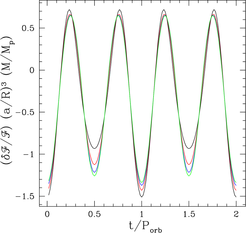
Figure 1.— Disk-averaged flux variation (eq. [16]) for an edge-on circular orbit under the equilibrium-tide approximation (eqs. [6] and [14]) with $\Delta F/F=0$ at the surface. The four curves correspond to $a/R=2$ (black), $4$ (red), $8$ (blue) and $16$ (green). In order to compare the shapes of the curves, $\delta\mathscr{F}/\mathscr{F}$ has been multiplied by $(a/R)^{3}(M/M_{p})$. As $a/R$ increases, higher harmonics decrease in strength and the lightcurve approaches a pure cosine with frequency $2/P_{\rm orb}$. The tidal bulge closest to the companion points toward the observer at integer values of $t/P_{\rm orb}$.

4. An Aside on von Zeipel’s Theorem

Our equilibrium calculation in the last section used the simple prescription $\Delta F_{\ell}/F=-\lambda_{\ell}\xi_{r,\ell}/R$. There remains the question of what physics determines $\Delta F/F$. A common practice in empirical studies of close eclipsing binaries—systems that tend to be nearly in tidal equilibrium—is to use some variant of the von Zeipel (1924) theorem, which was originally formulated for purely radiative, strictly hydrostatic stars. In equilibrium, all the thermodynamic variables depend only on the local value of the total potential $\Phi$. Thus, the radiative flux can be written as (e.g., Hansen & Kawaler, 1994)

$$\mathbf{F} \propto -\frac{1}{\kappa\rho}\frac{dT^{4}}{d\Phi}\boldsymbol{\nabla}\Phi~{},$$ (20)

where $\rho$ is the mass density, $T$ is the effective temperature, and $\kappa(\rho,T)$ is the opacity. Equation (20) is the essence of von Zeipel’s theorem, which says that the magnitude $F$ of the radiative flux is proportional to the magnitude of the net acceleration $A=|\boldsymbol{\nabla}\Phi|$. When $\Phi=\varphi+U$ (see § 3), we obtain $A=g+\partial U/\partial r+{\cal O}(\xi^{2})$, so that the Lagrangian flux perturbation about equilibrium is

$$\frac{\Delta F}{F}=\frac{\Delta A}{g}=\frac{\Delta g}{g}+\frac{1}{g}\frac{\partial U}{\partial r}~{},$$ (21)

where $\Delta g/g=-2\xi_{r}/r$, due to the change in radius at approximately constant enclosed mass. Substituting the equilibrium-tide result $U=-\xi_{r}g$ into eq. (21), we obtain the compact expression $\Delta F/F=-\partial\xi_{r}/\partial r$. Using eq. (14), we find

$$\frac{\Delta F_{\ell}}{F}=-(\ell+2)\frac{\xi_{r,\ell}}{r}~{},$$ (22)

from which we identify $\lambda_{\ell}=\ell+2$.

Although the application of von Zeipel’s theorem is instructive, the underlying physical assumptions are inaccurate for slowly rotating main-sequence stars of mass 1.0–$1.6\,M_{\odot}$ with tidal forcing periods of days. We are now led to investigate the general problem of forced nonadiabatic stellar oscillations.

5. FORCED NONADIABATIC OSCILLATIONS

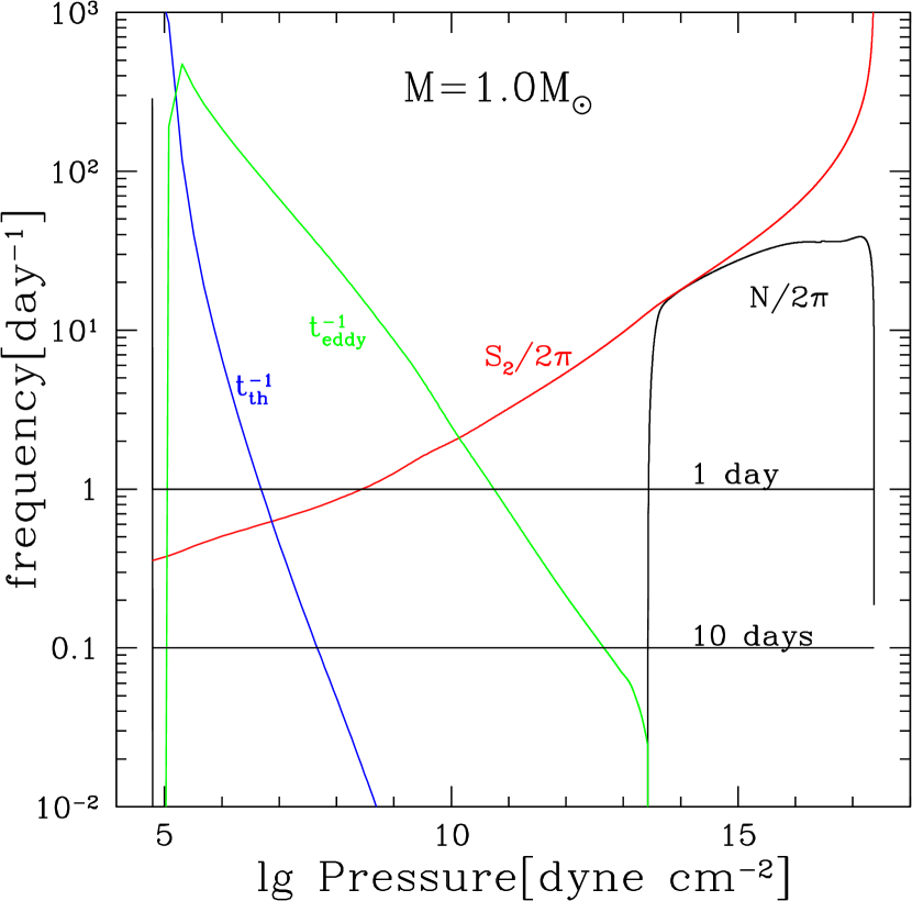
Figure 2.— Important oscillations frequencies and time scales as a function of pressure for a $1\,M_{\odot}$ main-sequence star. The four curves show the Brunt-Väisällä frequency $N$ (black), Lamb frequency $S_{l}$ (red; $\ell=2$ is shown), inverse thermal time $t_{\rm th}^{-1}$ (blue), and inverse eddy turnover time $t^{-1}_{\rm ed}$ (green). Large, real values of $N$ occur in the radiative core and very near the photosphere, while $N^{2}<0$ in the convective envelope. Gravity waves propagate only where the angular frequency is below both $N$ and $L_{\ell}$. The two horizontal lines delimit the range of tidal forcing frequencies of interest here.

The equilibrium analysis ignores fluid inertia and the excitation of the star’s natural oscillation modes. While this assumption may be valid near the surface of the star, it does not hold deeper in the interior. Gravity waves ($g$-modes; restored by buoyancy) can propagate in the radiative interiors of Sun-like stars with a range of oscillation periods that includes the tidal forcing periods of interest ($\lesssim$3 days). Tidal forcing of radiative regions may produce substantial deviations from hydrostatic balance, as well as large surface amplitudes of $\Delta F/F$, in particular if resonant oscillations are excited. This is especially relevant for main-sequence stars of mass $M\gtrsim 1.4$–$1.5\,M_{\odot}$ with mainly radiative envelopes. Less massive stars ($M\lesssim 1.3$–$1.4\,M_{\odot}$) have rather deep convective envelopes that can block information about the dynamic interior from being conveyed to the surface. Here we investigate each of these regimes with both analytic estimates and numerical models of oscillating stars.

Our calculations employ realistic models of 0.9–$1.6\,M_{\odot}$ main-sequence stars, constructed with the EZ stellar evolution code (Paxton, 2004), a distilled and rewritten version of the program originally created by Peter Eggleton. We adopt Solar metallicity and a convective mixing length of 1.6 times the pressure scale height. All stars are evolved to an age when the core hydrogen abundance has the Solar value of $X_{H}=0.35$. Models with 199 radial grid points are interpolated to yield $\gtrsim$$10^{4}$ points in which the $g$-mode radial wavelength is well resolved in the core.

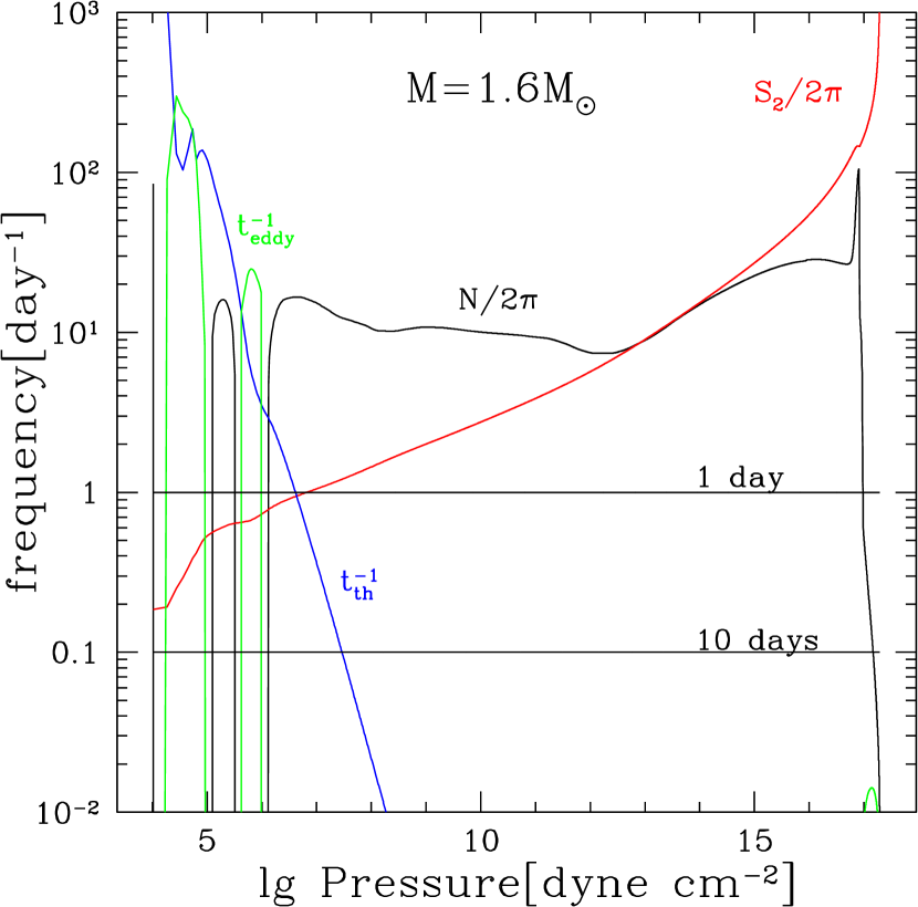
Figure 3.— Same as Fig. 2, but for a $1.6M_{\odot}$ main-sequence star. Note two geometrically thin, relatively inefficient ($t_{\rm th}\sim t_{\rm ed}$) convection zones near the surface. The spike in $N$ near the center is at the edge of the convective core, and signals a steep gradient in the mean molecular weight.

Figures 2 and 3 illustrate some of the differences between $1\,M_{\odot}$ and $1.6\,M_{\odot}$ stars, and serve to introduce several important physical quantities used in the remainder of this section. The Lamb frequency,

$$S_{\ell}=[\ell(\ell+1)]^{1/2}\frac{c_{s}}{r}~{},$$ (23)

is the inverse of the horizontal sound-crossing time scale, where $c_{s}$ is the sound speed, and $[\ell(\ell+1)]^{1/2}/r\equiv k_{h}$ is the horizontal wavenumber of the oscillation. For fixed chemical composition, the squared Brunt-Väisällä frequency is

$$N^{2}\simeq\frac{g}{H_{p}}(\nabla_{\rm ad}-\nabla)~{},$$ (24)

where $H_{p}=-(d\ln p/dr)^{-1}=p/(\rho g)$ is the pressure scale height, and $\nabla=d\ln T/d\ln p$ is the temperature gradient ($\nabla_{\rm ad}$ is the adiabatic value). Radiative regions have $\nabla_{\rm ad}-\nabla>0$ ($N^{2}>0$), and $N$ represents the frequency of buoyancy oscillations. In convection zones, $\nabla_{\rm ad}-\nabla<0$ and $N^{2}<0$, indicating that $g$-modes are evanescent. When $N^{2}<0$, the time scale

$$t_{\rm ed}\sim|N|^{-1}~{},$$ (25)

approximates the turnover time of convective motions (for details and modifications for radiative losses, see, e.g., Kippenhahn & Weigert 1990). A shell of radius $r$, thickness $H_{p}$ (size of the largest convective eddies), and radiative luminosity $L$ cools on the thermal time scale

$$t_{\rm th}=\frac{4\pi r^{2}H_{p}\rho C_{p}T}{L}~{},$$ (26)

where $C_{p}$ is the specific heat at constant pressure.

The $1\,M_{\odot}$ model (Fig. 2) has one deep convection zone with $t_{\rm ed}\ll t_{\rm th}$ over most of the region, indicating that convection very efficiently transports energy and causes the zone to be essentially isentropic. By consrast, the $1.6\,M_{\odot}$ star (Fig. 3) has two thin surface convection zones with $t_{\rm ed}\sim t_{\rm th}$, and thus the radiative and convective fluxes are comparable. Gravity waves with frequency $\omega$ propagate only in radiative regions where $\omega<N$ and $\omega<S_{\ell}$. For the $1\,M_{\odot}$ star, heat and entropy generated by $g$-modes in the radiative interior may be strongly mitigated owing to the long thermal time at the base of the deep convection zone. On the other hand, $g$-modes in a $1.6\,M_{\odot}$ star can propagate very near the surface, producing qualitatively different results.

We now go on to elucidate the physics of the flux perturbations. All the analytic and numerical work that follows assumes that the tidal potential has the generic form $U\propto r^{\ell}Y_{\ell m}(\theta,\phi)\exp(-i\omega t)$ with forcing frequency $\omega$.

Figure 4.— Eddy turnover time at base of the convective envelope versus stellar age for a range of stellar masses.

5.1. Heat Transfer in a Convective Envelope

Calculation of the perturbed convective flux in oscillating stars is a thorny issue. For the purposes of our study, we argue for an especially simple treatment that draws from previous work on this subject. Specifically, we modify the prescription of Brickhill (1983, 1990; see also Goldreich & Wu 1999a,b), which was originally applied to white-dwarf pulsations, into a form appropriate for the tidal flow problem.

In the mixing-length theory of convection, heat is transported by eddies with a spectrum of sizes $l\lesssim H_{p}$, speeds $v_{l}$, and turnover times $t_{\rm ed}(l)=l/v_{l}$. The Kolmogorov scalings for turbulent motions give $v_{l}\propto l^{1/3}$, $t_{\rm ed}\propto l^{2/3}$, and an energy density per unit mixing length interval $\propto$$l^{-1/3}$. We see that in the unperturbed star most of the convective energy flux ($\propto$$v_{l}^{3}$ at scale $l$) is carried by the largest eddies ($l\sim H_{p}$). Convection efficiently transports energy when the radiative thermal time scale associated with the dominant eddies is much longer than $t_{\rm ed}$. Alternatively, efficient convection implies that the gradient of the specific entropy $s$ is small; i.e., $d\ln s/d\ln p\ll 1$. If all the convective energy flux $F$ is carried by eddies with mixing length $l$, the flux and entropy gradient are related by (e.g., Kippenhahn & Weigert, 1990)

$$\frac{1}{C_{p}}\frac{ds}{d\ln p}(l) = \left(\nabla-\nabla_{\rm ad}\right)\sim\left[\frac{F}{pc_{s}}\left(\frac{H_{p}}{l}\right)^{2}\right]^{2/3}~{}.$$ (27)

Efficient convection enforces $\nabla-\nabla_{\rm ad}\ll 1$, which implies $d\ln s/d\ln p\ll 1$, since $s\gtrsim C_{p}$ in the convective regions of our background models.

Figure 5.— Thermal time at the base of the convection envelope versus stellar age for a range of stellar masses.

Gravity waves with the tidal forcing frequency $\omega$ are excited in the radiative region below the convection zone. Convective eddies can transport heat during a forcing period only if $t_{\rm ed}<2\pi/\omega$ (e.g., Brickhill, 1990; Goldreich & Wu, 1999b). Inspection of Fig.  2 shows that in the $1\,M_{\odot}$ model, the largest eddies have $t_{\rm ed}\simeq 20(p/p_{\rm bcz})^{0.5}$ days, where $p_{\rm bcz}\simeq 10^{13.5}\ {\rm dyne\ cm^{-2}}$ is the pressure at the base of convection zone. Using the Kolmogorov scaling, the “resonant” length $l_{\rm res}$ for which $\omega t_{\rm ed}/2\pi=1$ is

$$\frac{l_{\rm res}}{H_{p}} \sim 10^{-2}\ \left(\frac{2\pi/\omega}{1\ {\rm day}}\right)^{3/2}\left(\frac{p_{\rm bcz}}{p}\right)^{3/4}~{},$$ (28)

which is $>$1 for all periods $2\pi/\omega>1$ day when $p\lesssim 10^{12}\ {\rm dyne\ cm^{-2}}$, which still encompasses much of the convection zone. Now imagine the situation where all the convective flux is carried by eddies of size $\lesssim$$l_{\rm res}$. The entropy gradient for this range of mixing lengths is

$$\frac{1}{C_{p}}\frac{ds}{d\ln p}(l_{\rm res}) \sim 10^{-3}\left(\frac{2\pi/\omega}{1\ {\rm day}}\right)^{-1}\left(\frac{p}{p_{\rm bcz}}\right)~{},$$ (29)

where we have adopted $F/pc_{s}\sim 10^{-8}$ at the base of the convection zone, as indicated by our $1\,M_{\odot}$ stellar model.

These arguments suggest that convection is efficient in a $1\,M_{\odot}$ star at the forcing periods of interest even if small “resonant” eddies carry all the energy flux near the base of the convection zone. At larger radii, but not too near the photosphere, convection is both efficient and rapid ($\omega t_{\rm ed}/2\pi<1$) over the full spectrum of eddies. Rapid convection on all scales $l\lesssim H_{p}$ enforces isentropy in the convection zone, such that $s$ and its Lagrangian perturbation $\Delta s$ are nearly constant, as in the Brickhill (1983, 1990) picture. While convection at the base is rapid only on small scales, it is still highly efficient, which yields $s\simeq\textrm{constant}$ and further indicates that $\Delta s/C_{p}$ is small in magnitude, as we demonstrate in § 5.2.

As the stellar mass increases, the convection zone thins and $t_{\rm ed}$ at the base decreases (see Figs. 3 and 4). Rapid convection holds over the bulk of the convection zone for masses $\gtrsim$$1\,M_{\odot}$. However, the assumption that the convection is efficient starts to break down at 1.4–$1.5\,M_{\odot}$, since $t_{\rm th}\sim t_{\rm ed}$ at the base (see Figs. 3 and 5). For the full range of stellar masses considered here, we assume that $s$ and $\Delta s$ are constant in convection zones.

5.2. Analytic Result for Thick Convection Zones

In a fully convective star, the emergent luminosity is determined entirely by the surface boundary conditions. Under our assumption that $\Delta s$ is constant in the convection zone, the perturbed luminosity is likewise a function only of the boundary conditions. Stars of mass $\lesssim$1.3–$1.4\,M_{\odot}$ have long thermal times ($\omega t_{\rm th}\gg 1$) at the top of the interior radiative region (see Fig. 5), so that the flux perturbation $\Delta F$ is approximately the “quasi-adiabatic” value, derived by ignoring $\Delta s\propto(\omega t_{\rm th})^{-1}$ in eq. (A5). We assume efficient convection continues to just below the photosphere.

At the photosphere, we adopt the usual Stefan-Boltzmann relation, $F=\sigma T^{4}$, and the hydrostatic condition, $p\kappa/A=2/3$, where $A$ is the total acceleration defined in § 4, and 2/3 is the photospheric optical depth. Taking the photosphere to define the stellar surface, we compute the Lagrangian perturbations,

$$\frac{\Delta F}{F}=4\frac{\Delta T}{T}~{},$$ (30)

and

$$\frac{\Delta p}{p}-\frac{\Delta A}{g}+\frac{\Delta\kappa}{\kappa}=0~{}.$$ (31)

Using $s$ and $p$ as our independent thermodynamic variables, we write $\Delta\kappa/\kappa=\kappa_{\rm ad}\Delta p/p+\kappa_{s}\Delta s/C_{p}$ and $\Delta T/T=\Delta s/C_{p}+\nabla_{\rm ad}\Delta p/p$. In our numerical work (see § 5.4), we self-consistently compute the perturbation $\Delta A$ to the effective surface gravity, in order to follow resonant oscillations, where the equilibrium-tide result fails. However, we are now addressing non-resonant forcing, for which we use the equilibrium-tide approximation at the surface, giving $\Delta A/g=-\partial\xi_{r}/\partial r$ (see § 4). We now have

$$\frac{\Delta p}{p} = -\left(\frac{\kappa_{s}\Delta s/C_{p}+\partial\xi_{r}/\partial r}{1+\kappa_{\rm ad}}\right)~{},$$ (32)

and upon substitution,

$$\frac{\Delta F}{F}=4\left(\frac{1+\kappa_{\rm ad}-\nabla_{\rm ad}\kappa_{s}}{1+\kappa_{\rm ad}}\right)\frac{\Delta s}{C_{p}}-\frac{4\nabla_{\rm ad}}{1+\kappa_{\rm ad}}\frac{\partial\xi_{r}}{\partial r}~{}.$$ (33)

Equation (33) differs from Goldreich & Wu (1999a) in that we retain the gravity perturbation in eq. (31), whereas they consider a constant-gravity atmosphere (and no tidal perturbation). For $g$-modes in white dwarfs, the interesting region is near the surface and the motion is mainly horizontal, so that $\Delta A=\Delta g=0$ is a good approximation. Since the equilibrium tide has large vertical motions, the $\Delta A$ term must be retained.

The luminosity change across the convection zone is derived from the entropy equation (eq. [A6]). If we ignore horizontal flux perturbations (set $\ell=0$ in eq. [A6]) and energy generation, the equation for the luminosity perturbation $\Delta L/L=2\xi_{r}/r+\Delta F/F$ is

$$\frac{d(\Delta L/L)}{dM_{r}} = i\omega T\Delta s/L~{}.$$ (34)

Integrating over the convection zone with constant $\Delta s$, we obtain

$$\frac{\Delta L_{\rm ph}}{L}-\frac{\Delta L_{\rm bcz}}{L}=i\omega\Delta s\int_{\rm cz}dM_{r}T/L~{},$$ (35)

where the subscript “ph” refers to the photosphere. We define $t_{\rm cz}=C_{p,{\rm ph}}\int_{\rm cz}dM_{r}T/L$ to be the mean thermal time of the convection zone, so that the right-hand side of eq. (35) is $i\omega t_{\rm cz}\Delta s/C_{p,{\rm ph}}$.

Figure 5 shows that the thermal time at the base of the convection zone (of order $t_{\rm cz}$) for $M\lesssim 1.3\,M_{\odot}$ is orders of magnitude longer than the forcing periods of 1–10 days. Insofar as $|\Delta L|/L\sim|\xi_{r}|/r$ at any location in the star (i.e., if resonances are neglected), we see that $(|\xi_{r}|/r)^{-1}|\Delta s|/C_{p}\sim(\omega t_{\rm cz})^{-1}\ll 1$ in stars with deep convective envelopes. In this limit, eq. (33) becomes

$$\frac{\Delta F}{F}\simeq-\frac{4\nabla_{\rm ad}}{1+\kappa_{\rm ad}}\frac{\partial\xi_{r}}{\partial r}~{}.$$ (36)

If we had set $\Delta A=0$, the amplitude of the photospheric flux perturbation would have been $\sim$$|\Delta s|/C_{p}$ rather than the much larger value $\sim$$|\xi_{r}|/R$.

Photospheric flux perturbations in tidally forced solar-type stars with thick convective envelopes arise mainly from changes in the local effective gravity. This statement is reminiscent of, but physically distinct from, von Zeipel’s theorem (eqs. [21] and [22]). We have recovered our equilibrium-tide scaling, $\Delta F_{\ell}/F=-\lambda_{\ell}\xi_{r,\ell}/R$, where eq. (36) gives

$$\lambda_{\ell}=4(\ell+2)\frac{\nabla_{\rm ad}}{1+\kappa_{\rm ad}}~{}.$$ (37)

For $M=1.0$–$1.4\,M_{\odot}$, we find $\lambda_{2}\simeq 1.9$–1.1. These estimates neglect resonant excitation of $g$-modes, a point addressed in § 5.4.

5.3. Analytic Result for Radiative Envelopes

As the stellar mass increases beyond $1.4\,M_{\odot}$, the outer convective region thins and sits close to the surface, where $t_{\rm ed}\sim t_{\rm th}$. Figure 3 shows that the $1.6\,M_{\odot}$ model has two thin, inefficient surface convection zones, as well as a convective core. Radiative energy transport is important throughout the envelopes of these more massive stars. We now consider the idealized case of a completely radiative envelope, and obtain an analytic approximation for $\Delta L/L$ at the surface.

Near the surface of a radiative star, we have $H_{p}/r\ll 1$, $4\pi r^{3}\rho/M_{r}\ll 1$, and $\omega^{2}r/g\ll 1$ for $2\pi/\omega=1$–10 days. Under these conditions, the quasi-adiabatic luminosity perturbation becomes (e.g., Unno et al., 1989)

$$\frac{\Delta L_{\rm qad}}{L}\simeq-\zeta\frac{\Delta p}{p}+\frac{gk_{h}^{2}H_{p}}{\omega^{2}}\left(\frac{\nabla_{\rm ad}}{\nabla}-1\right)\left(\frac{\Delta p}{p}+\frac{\xi_{r}-\xi_{r,\rm eq}}{H_{p}}\right)$$

(38)

where

$$\zeta=\kappa_{\rm ad}-4\nabla_{\rm ad}+\frac{\nabla_{\rm ad}}{\nabla}-\frac{d\nabla_{\rm ad}}{d\ln T}~{},$$ (39)

and $\xi_{r,\rm eq}$ is the equilibrium-tide radial displacement (eq. [12]). Nonzero values of $\Delta p/p$ and $(\xi_{r}-\xi_{r,{\rm eq}})/H_{p}$ indicate deviations from hydrostatic equilibrium. Care must be taken with these terms, because the denominators $p$ and $H_{p}$ become very small close to the surface.

With the help of the Appendix, we define the variables

$$\alpha = y_{1}-y_{2}+y_{3}=-\frac{H_{p}}{r}\frac{\Delta p}{p}~{},$$ (40)

$$\beta = y_{2}+\frac{U}{gr}=\frac{H_{p}}{r}\frac{\Delta p}{p}+\frac{\xi_{r}-\xi_{r,\rm eq}}{r}~{},$$ (41)

which satisfy the differential equations

$$\frac{d\alpha}{dr} \simeq -\frac{d\ln\rho}{dr}\alpha+\frac{gk_{h}^{2}}{\omega^{2}}\beta+(\ell+4)\frac{U}{gr^{2}}~{},$$ (42)

$$\frac{d\beta}{dr} = -\frac{N^{2}}{g}\alpha+\frac{\beta}{r}~{}.$$ (43)

When $\omega^{2}\ll gk_{h}^{2}H_{p}$, these equations produce the $g$-mode dispersion relation $k_{r}^{2}=k_{h}^{2}N^{2}/\omega^{2}$ (in the limit $k_{r}^{2}/k_{h}^{2}\ll 1$) for radial wavenumber $k_{r}$. For these propagating waves, the surface amplitudes of $\alpha$ and $\beta$ are determined at the core radiative-convective boundary, where $g$-modes are driven (e.g., Goldreich & Nicholson, 1989). On the other hand, when $\omega^{2}\gg gk_{h}^{2}H_{p}$, the $g$-modes are evanescent (see Unno et al., 1989) and we neglect the term $gk_{h}^{2}\beta/\omega^{2}$ in eq. (42). This limit yields the approximate solution $\alpha\simeq-(\ell+4)(H_{p}U/gR^{2})$, or $\Delta p/p\simeq(4+\ell)U/gR$. In this case, $\Delta p/p$ is not small compared to the fractional fluid displacement, and thus the equilibrium-tide approximation loses validity.

From our stellar models, we find that the evanescent regime corresponds to forcing periods of $\lesssim$4–8 days for $M=1$–$1.6\,M_{\odot}$, most of the range of interest. The high-frequency limit of eq. (38) is

$$\frac{\Delta L_{\rm qad}}{L}\simeq-\zeta(\ell+4)\ \frac{U}{gR}~{}.$$ (44)

This relation should be evaluated at the layer where $\omega t_{\rm th}\simeq 1$, above which the luminosity effectively “freezes out.” Figure 6 shows the quasi-adiabic flux perturbation $\Delta F_{\rm qad}/F=\Delta L_{\rm qad}/L-2\xi_{r}/R$, evaluated where $\omega t_{\rm th}=1$, for a range of forcing periods and $M=1.5$–$1.7\,M_{\odot}$. Note that $|\Delta F/F|$ can be an order of magnitude larger than $|U|/gR$, because of the rather large values of $|\zeta|(\ell+4)$ for $\ell\geq 2$. Much larger perturbations are possible when $g$-modes are resonantly excited in a radiative star, as we discuss in the next section.

We must point out that the quasi-adiabatic approximation is technically inappropriate when $\omega t_{\rm th}\sim 1$. Equation (44) should be viewed as an estimate of the modulus of the luminosity perturbation at the surface. If, for instance, $|\Delta s|/C_{p}\gtrsim|U|/gR$ where $\omega t_{\rm th}\sim 1$, then $\Delta L/L$ at the surface will have a substantial imaginary part (see eq. [34]). This is what we find in the numerical calculations summarized in the next section.

Figure 6.— Ratio of surface Lagrangian flux perturbation $\Delta F/F$ to equilibrium-tide displacement $-U/gR$ for a range of forcing periods in the limit where surface $g$-modes are evanescent. The flux is evaluated at the location where $\omega t_{\rm th}=1$. Dashed, solid, and dotted curves correspond to $M=1.5$, 1.6, and $1.7\,M_{\odot}$, respectively.

5.4. Numerical Examples

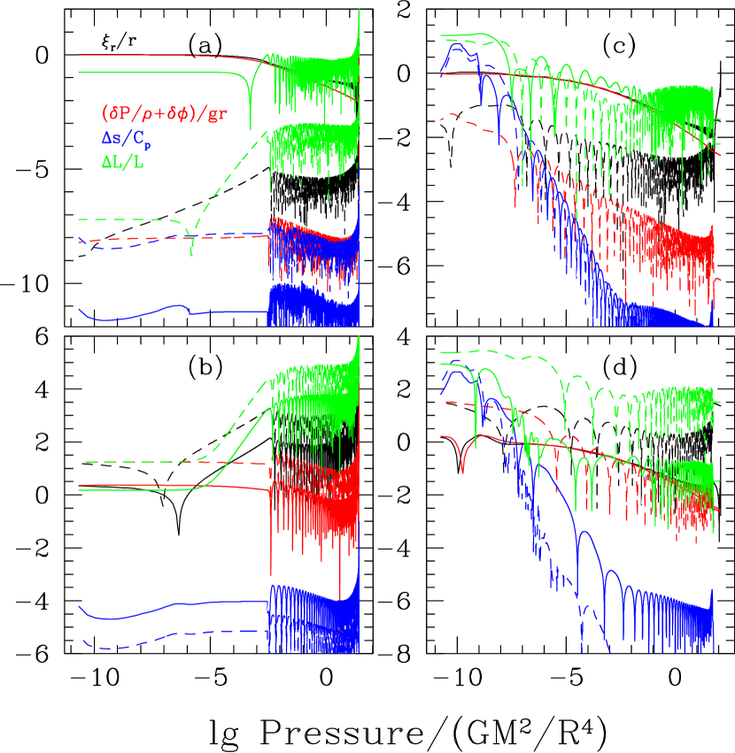
Figure 7.— Responses of tidally forced $1\,M_{\odot}$ and $1.6\,M_{\odot}$ main-sequence stars. Black, red, blue, and green curves denote, respectively, the logarithms of $\xi_{r}/r$, $(\delta p+\rho\delta\varphi)/\rho gr$, $\Delta s/C_{p}$, and $\Delta L/L$. Solid (dashed) curves show the real (imaginary) parts. The tidal potential has been scaled so that $\xi_{r}/R=1$ corresponds to the equilibrium-tide value. The four panels show the following: (a) non-resonant response of a $1\,M_{\odot}$ star tidally forced at a period of $2\pi/\omega\simeq 2.91\,{\rm day}$; (b) resonant response of a $1\,M_{\odot}$ star with $2\pi/\omega\simeq 1.00\,{\rm day}$; (c) non-resonant response of a $1.6\,M_{\odot}$ star with $2\pi/\omega\simeq 3.00\,{\rm day}$; (d) resonant response of a $1.6\,M_{\odot}$ star with $2\pi/\omega\simeq 1.02\,{\rm day}$

Here we show solutions of the perturbed mass, momentum, and energy equations that describe linear, nonadiabatic oscillations of a star subject to a varying tidal force. The equations listed in the Appendix are the same as in Unno et al. (1989) for radiative regions, but augmented to include the tidal acceleration. In convection zones, we apply the prescription $\Delta s=\textrm{constant}$ based on our conclusions in § 5.1. Figure 7 summarizes how the interiors of $1\,M_{\odot}$ and $1.6\,M_{\odot}$ stars respond to resonant and non-resonant tidal forcing. The tidal potential has been scaled so that $\xi_{r}/R=1$ corresponds to the equilibrium-tide surface displacement.

For our $1\,M_{\odot}$ model, the non-resonant response to a forcing period of $\simeq$3 days is shown in Fig. 7a. We see that $\xi_{r}/R$ matches the equilibrium-tide result at the surface; the imaginary piece is completely negligible. We also find that our approximation for $\Delta F/F$ at the surface (eq. [36]) works very well. A factor of $\sim$10 decay in $|\Delta L|/L$ occurred in order for $|\Delta F|/F\sim\xi_{r}/R$ at the surface. Variation of $\Delta s/C_{p}$ in the convection zone ($\log[p/(GM^{2}/R^{4})]>-2.5$) is due to changes in $C_{p}$. In the radiative interior, the oscillations are caused by most nearly resonant $g$-modes, whose amplitudes rise rapidly as the core is approached, due to conservation of wave luminosity. We have checked that the quasi-adiabatic approximation of $\Delta L/L$ is valid in the radiative region; the ratio of the real and imaginary parts is found to be roughly constant for the ingoing gravity-wave (see also Zahn, 1975).

In order to model the resonant response of a $1\,M_{\odot}$ star, we tuned the forcing period to $\simeq$1 day (see Figs. 7b and 8). At the surface, both $\xi_{r}$ and $\Delta L$ have dominant imaginary parts, due to the short radial wavelength of the $g$-mode compared to the equilibrium-tide fluid displacement. The entropy at the base of the convection zone is very strongly perturbed in comparison to the non-resonant case, but $\Delta L$ is still damped by orders of magnitude as the surface is approached.

Figure 8 shows the surface values of the complex modulus and phase of $\xi_{r}/R$ and $\Delta F/F$ versus forcing period. The phase is $\tan^{-1}(\textrm{Imaginary/Real})\in(-\pi,\pi)$. Solid lines connect points halfway between $g$-mode resonant periods. We find that the equilibrium-tide approximation given by eqs. (12) and (36) is excellent for non-resonant forcing. Dashed curves give the maximum and minimum values that occur on resonance. One example of a resonance is shown in the insets. Resonant forcing at periods of $<$2 days yields surface values of $\xi_{r}/R$ and $\Delta F/F$ that differ substantially from the equilibrium-tide results. However, the ratio of resonance width to the spacing between adjacent resonances is $\sim$$10^{-4}$, making resonant forcing very unlikely. It is noteworthy that at forcing periods of $>$2 days, the equilibrium-tide result holds extremely well even when precisely on a resonance. As explained by Zahn (1975), the resonant response can be considered as the sum of the equilibrium tide and the most nearly resonant wave. As the period increases, the $g$-mode radial wavelength decreases, resulting in a reduction of the overlap integral for the mode and the tidal force, which in turn gives a decreased amplitude of the wave component relative to the equilibrium tide.

The non-resonant response of the $1.6\,M_{\odot}$ star is shown in Fig. 7c. We see that the equilibrium-tide result provides a good match to $\xi_{r}/R$. Our estimate for the modulus of the radiative luminosity perturbation in the evanescent limit (eq. [44]) agrees reasonably well with what is in Fig. 7c. We also see that $\Delta L/L$ does roughly “freeze-out” when $\omega t_{\rm th}\simeq 1$, just below the base of the convection zone at $\log p/(GM^{2}/R^{4})\simeq-9$ (see Fig. 3). Our expectations in § 5.3 regarding the imaginary part of $\Delta L/L$ are borne out in Fig. 7c

A resonantly excited $1.6\,M_{\odot}$ star exhibits huge surface flux perturbations, radial displacements, and phase lags, as seen in Fig. 7d. In Fig. 9, surface values of $|\xi_{r}|/R$ and $|\Delta F|/F$ are plotted as a function of forcing period, where we have taken care to resolve resonances. Resonant amplitudes vary non-monotonically with period, in contrast to the smooth behavior of the $1\,M_{\odot}$ star (Fig. 8). Although we do not show the results here, similar plots for masses between $1\,M_{\odot}$ and $1.6\,M_{\odot}$ show progressively more structure as the mass increases. The cause of this irregularity is not clear, but may have to do with the two thin surface convection zones changing the overlap of successive $g$-modes with the tidal force.

Figure 8.— Surface radial displacement and Lagrangian flux perturbation versus forcing period for a $1.0M_{\odot}$ star. Solid lines connect points halfway between resonant $g$-mode periods, while dashed curves give the maximum and minimum values found on resonance. The equilibrium-tide approximation is extremely good, except when the forcing period is $<$2 days and resonant.

6. SUMMARY

We have investigated in detail the ellipsoidal oscillations of 0.9–$1.6\,M_{\odot}$ main-sequence stars induced by substellar companions. Classical models of ellipsoidal variability (e.g., Wilson, 1994) are built on the assumption of hydrostatic balance in a frame corotating with the binary orbit. This approach is justified in the context of short-period ($P_{\rm orb}\lesssim 10$ days) binaries containing two stars of comparable mass, where tidal dissipation circularizes the orbits and synchronizes the stellar spins with the orbital frequency. However, when the companion has a very low mass, we cannot assume that the binary is in complete tidal equilibrium; in fact, this state may be unattainable (see § 2). In this case, one must, in general, appeal to a dynamical description of the tidal interaction. A substellar companion with $P_{\rm orb}\gtrsim 1$ day raises tides on the star that are a small fraction of the stellar radius (see eq. [1]), permitting a linear analysis of the stellar oscillations.

While the root of our study is a dynamical treatment of stellar tidal perturbations, the equilibrium-tide approximation does have an important realm of validity (see below). For this reason, we derived in § 3 a general expression (eq. [16]) for the measurable flux variation of a star that remains in hydrostatic equilibrium under the influence of a small external tidal force. This formula (1) assumes that the local perturbation to the energy flux at the stellar surface is proportional to and in phase with the equilibrium-tide radial fluid displacement at each angular order $\ell$ (eq. [12]), (2) neglects stellar rotation, and (3) applies to inclined and eccentric orbits. As expected, the fractional amplitude of the modulation is $\sim$$\varepsilon\equiv(M_{p}/M)(R/a)^{3}$ for small eccentricities and $I=90^{\circ}$, or $\sim$$10^{-5}(M_{p}/M_{J})(P_{\rm orb}/1\,{\rm day})^{-2}$ for a star like the Sun (see § 2).

Figure 9.— Surface radial displacement and Lagrangian flux perturbation versus forcing period for a $1.6M_{\odot}$ star. Curves connect evenly spaced points away from resonances, with finer spacing near resonance periods.

A common practice is to use von Zeipel’s theorem when computing the surface radiative flux from a tidally distorted star (see § 4). The theorem assumes that the star is in hydrostatic equilibrium and that the energy transport in the outer layers is purely by radiative diffusion. As already mentioned, the hydrostatic assumption is technically unjustified for substellar perturbers. Moreover, the majority of Kepler targets will be main-sequence stars with masses of $<$$1.4\,M_{\odot}$, which have substantial surface convection zones. Evidently, von Zeipel’s theorem is an inappropriate starting point for the conditions of interest.

Section 5.1 discusses heat transport in perturbed stars with convective envelopes. Heuristic arguments are used to develop a simple treatment of the perturbed convection zone in main-sequence stars of mass $<$$1.6\,M_{\odot}$ with forcing periods of 1–10 days. We suggest that both the specific entropy $s$ and its Lagrangian perturbation $\Delta s$ are spatially constant in convective regions, a model partly inspired by the ideas of Brickhill (1983, 1990).

Table 2Periodic Flux Modulations

Variability		Dominant	Phase at
Source	Amplitude	Harmonic	Maximum/Minimum	References
Ellipsoidal	$2\times 10^{-5}m_{p}mP_{1}^{-2}\sin^{2}I$	$P_{\rm orb}/2$	0.25(0.75)/0.00(0.50)	$\cdots$
Doppler	$3\times 10^{-6}m_{p}m^{-2/3}P_{1}^{-1/2}\sin I$	$P_{\rm orb}$	0.25/0.75	1
Reflection	$6\times 10^{-5}(\alpha/0.1)m^{-2/3}P_{1}^{-4/3}\sin I$	$P_{\rm orb}$	0.50/0.00	2,3
Transit	$10^{-2}m^{-2}$	$P_{\rm orb}$	$\cdots$ /0.00	4

References. — (1) Loeb & Gaudi 2003; (2) Seager, Whitney, & Sasselov 2000; (3) Sudarsky, Burrows, & Pinto 2000; (4) Seager & Mallén-Ornelas 2003

Using this prescription, we analytically compute in § 5.2 the perturbed flux at the photosphere of deeply convective stars ($M\lesssim 1.4\,M_{\odot}$), where the thermal time scale at the base of the convection zone is much longer than the forcing period. We find that $\Delta s/C_{p}$ is negligible near the top of the convection zone, and that the photospheric flux perturbation is proportional to changes in the effective surface gravity. Thus, we recover the equilibrium-tide result, $\Delta F/F=-\lambda_{\ell}\xi_{r}/R$, at the surface, where $\lambda_{\ell}$ depends on the adiabatic derivatives of opacity and temperature with respect to pressure (see eq. [37]). Numerical solutions of the equations of linear, nonadiabatic stellar oscillations (see § 5.4 and Fig. 7a) corroborate our analytic estimates in the non-resonant regime. Resonant excitations of $g$-modes in the radiative stellar interior cause large departures from the equilibrium-tide approximation when the forcing period is $<$2 days (Figs. 7b and 8). However, the likelihood of being on a resonance is small, and at periods of $>$2 day the equilibrium-tide result holds for $M\simeq 1\,M_{\odot}$ even with resonant forcing.

Stars of mass $\gtrsim$$1.4\,M_{\odot}$ have thin, relatively inefficient surface convection zones. Thus, $g$-modes can propagate very close to the surface and produce large flux perturbations and fluid displacements. Analytic arguments in § 5.3 indicate that the surface flux perturbations in these stars have non-resonant amplitudes of $\sim$$10\varepsilon$ (eq. [44] and Fig. 6), in rough agreement with our numerical calculations (Fig. 7c). As seen in Figs. 7d and 9, a resonantly forced $1.6\,M_{\odot}$ star can exhibit flux perturbation amplitudes of $>$$100\varepsilon$ at forcing periods of $\simeq$1 day. While the amplitudes are not as extreme at longer periods, their dependence on period is rather erratic (Fig. 9), an issue that deserves further study. It will be difficult to derive physical interpretations from the ellipsoidal variability of these more massive stars.

7. DETECTION PROSPECTS

The dominant sources of periodic variability of a star with a substellar companion are transit occultations (when $|\cos I|<[R+R_{p}]/a$), Doppler flux modulations, reflection of starlight from the companion, and ellipsoidal oscillations. For each of these signals, Table  6 lists the characteristic amplitude, period with the largest power in the Fourier spectrum, and orbital phase(s) at which the light is a maximum or minimum. The transit contribution is included for completeness, but its duration is sufficiently short—a fraction $\simeq$$(R+R_{p})/(\pi a)$ of $P_{\rm orb}$—that it should often be possible to excise it from the data (see Sirko & Paczyński, 2003). Of the remaining signals, the Doppler variability is the simplest, being purely sinusoidal with period $P_{\rm orb}$ when the orbit is circular. The dominant $\ell=2$ piece of the equilibrium-tide approximation to the ellipsoidal variability (see eqs. [16] and [17]) is also sinusoidal when $e=0$, but with period $P_{\rm orb}/2$. Reflection is more problematic, as its time dependence is generally not sinusoidal and not known a priori.

If the companion scatters light as a Lambert sphere (e.g., Seager et al., 2000), the Fourier spectrum of the reflection variability has finite amplitude at all harmonics of the orbital frequency $\Omega$, but the amplitude at $2\Omega$ is roughly 1/5 of the amplitude at $\Omega$. Therefore, the reflection and ellipsoidal variability amplitudes may be similar at a frequency of $2\Omega$ when $\alpha=0.1$, $M_{p}\sim M_{J}$, and $P_{\rm orb}\simeq 1$ day. Also, the orbital phase at which the reflected light is a maximum is distinct from both the Doppler and ellipsoidal cases, further distinguishing the signals. However, Lambert scattering is probably never appropriate in real planetary atmospheres. Infrared reemission of absorbed optical light, multiple photon scattering, and anisotropic scattering typically conspire to narrow the peak in the reflection lightcurve and lower the albedo, decreasing the prominence of the reflection signal. These issues are sensitive to the atmospheric chemistry and the uncertain details in models of irradiated giant planets. For reasonable choices regarding the atmospheric composition, calculated optical albedos of Jovian planets range from $<$0.01 to $\simeq$0.5 (Seager et al., 2000; Sudarsky et al., 2000). Recent photometric observations of HD 209458, the star hosting the first-detected transiting giant planet ($P_{\rm orb}\simeq 3.5$ days), constrain the planetary albedo to be $<$0.25 (Rowe et al., 2006).

Detailed lightcurve simulations will be required to say how well the different periodic signals can be extracted from the data. This is beyond the scope of the current study. We now do the simpler exercise of isolating the ellipsoidal modulations and assessing when this effect alone should be detectable. For a star of apparent visual magnitude $V$ and an integration time of $T=6\,{\rm hr}$, Kepler’s photon shot noise is

$$\left(\frac{\delta\mathscr{F}}{\mathscr{F}}\right)_{\rm shot}\sim 10^{-5}10^{0.2(V-12)}\left(\frac{T}{6\,{\rm hr}}\right)^{-1/2}~{}.$$ (45)

Instrumental noise should contribute at a similar level (e.g., Koch et al., 2006). If the data is folded at the orbital period and binned in time intervals $T\ll P_{\rm orb}$, the shot noise is suppressed by a factor of $\sim$$n_{\rm orb}^{-1/2}$, where $n_{\rm orb}$ is the number of folded cycles. After folding 1 year of continuous photometric data using $T=6$ hr, a star with $V<12$ orbited by a giant planet with $P_{\rm orb}\lesssim 3$ days may have a fractional shot noise per time bin of $\lesssim$$10^{-6}$. This is less than the ellipsoidal amplitude, $(\delta\mathscr{F}/\mathscr{F})_{\rm ell}$, when $I$ is not too small.

The actual situation is not so simple when the data spans of weeks or months, because the intrinsic stochastic variability of the star will not have a white-noise power spectrum. Over times of $\lesssim$1 day, the Sun shows variability of $(\delta\mathscr{F}/\mathscr{F})_{\rm int}\sim 10^{-5}$, but the amplitude rises steeply between $\sim$1 and 10 days to $\sim$$10^{-3}$. Intrinsic variability tends to be large near the rotation period of the star, due mainly to starspots. Low-frequency variability may not too damaging for the study of ellipsoidal oscillations induced by planets with $P_{\rm orb}\lesssim 3$ days, but more study is needed.

Kepler’s target list will contain $\simeq$$10^{5}$ main-sequence FGK stars with $V=8$–14. The statistics of known exoplanets indicate that 1–2% of all such stars host a giant planet ($M_{p}\gtrsim M_{J}$) with $P_{\rm orb}<10$ days (e.g., Marcy et al., 2005). Of these “hot Jupiters,” $\simeq$30% have $P_{\rm orb}=1$–3 days. It seems that a maximum of $\sim$$10^{3}$ Kepler stars will have detectable ellipsoidal modulations. If we neglect intrinsic stellar variability and consider only shot noise, then many systems with $P_{\rm orb}\lesssim 3$ days and $V<14$ will have signal-to-noise $S/N>1$ after $\sim$100 cycles are monitored; this may amount to $>$100 stars. Obviously, the number drops when we place higher demands on $S/N$ and include the intrinsic variability. The results depend critically on the distributions of $M_{p}$ and $P_{\rm orb}$.

In order to better estimate the number of stars with potentially detectable ellipsoidal oscillation, we perform a simple population synthesis calculation. Denote the set of star-planet system parameters by $\mathbf{P}=\{M,M_{p},P_{\rm orb},I\}$, and let $f(\mathbf{P})d\mathbf{P}$ be the probability of having a system in the 4-dimensional volume $d\mathbf{P}$. We assume that the planetary orbits are circular and obtain $(\delta\mathscr{F}/\mathscr{F})_{\rm ell}$ from the equilibrium-tide estimate in Table 6. Given the mass of the star, we compute its absolute $V$ magnitude on the main-sequence using the approximation (see also Henry & McCarthy, 1993)

$$\mathscr{M}_{V}=4.8-10.3\log(M/M_{\odot})~{},$$ (46)

which is in accord with the usual mass-luminosity relation $\log(L/L_{\odot})\simeq 4\log(M/M_{\odot})$ for $M\simeq 1\,M_{\odot}$. With a maximum apparent magnitude of $V_{\rm max}=14$ for the Kepler targets, the maximum distance of the star is

$$D_{\rm max}=10^{1+0.2(14-\mathscr{M}_{V})}\,{\rm pc}~{}.$$ (47)

With a certain signal-to-noise threshold $(S/N)_{\rm min}$, there is a maximum distance $D_{d}<D_{\rm max}$ to which the ellipsoidal variability is detectable. For a spatially uniform population, the detectable fraction of systems is $(D_{d}/D_{\rm max})^{3}$. Thus, the net detectable fraction among all systems is

$$\mathscr{E}=\int d\mathbf{P}f(\mathbf{P})\left(\frac{D_{d}}{D_{\rm max}}\right)^{3}~{},$$ (48)

an integral over all relevant $\mathbf{P}$ space.

When the only noise is intrinsic to the star, $N=(\delta\mathscr{F}/\mathscr{F})_{\rm int}$ and $S/N$ is independent of distance, so that $D_{d,{\rm int}}=D_{\rm max}$ when $S/N>(S/N)_{\rm min}$, and $D_{d,{\rm int}}=0$ otherwise. In the case of pure shot noise, there is a maximum magnitude $V_{d}$ for which the ellipsoidal oscillations are detectable:

$$V_{d}=5\log\left[\frac{(\delta\mathscr{F}/\mathscr{F})_{\rm ell}}{\chi\ (S/N)_{\rm min}}\right]~{},$$ (49)

where $\chi\sim 10^{-8.4}(T_{6}n_{100})^{-1/2}$ is the value of $(\delta\mathscr{F}/\mathscr{F})_{\rm shot}$ for $V=0$, $T=6T_{6}\,{\rm hr}$, and $n_{\rm orb}=100n_{100}$. The corresponding distance is given by $\log[D_{d,{\rm shot}}/10\,{\rm pc}]=0.2(V_{d}-\mathscr{M}_{V})$ if $V_{d}<V_{\rm max}$, and is $D_{d,{\rm shot}}=D_{\rm max}$ when $V_{d}>V_{\rm max}$. We take the maximum detectable distance to be $D_{d}=\min\{D_{d,{\rm int}},D_{d,{\rm shot}}\}$.

Table 3Number of Kepler Stars with Detectable Ellipsoidal Oscillations

		$(S/N)_{\rm min}=1$			$(S/N)_{\rm min}=3$			$(S/N)_{\rm min}=5$
$y$		$x=1$	$2$		$x=1$	$2$		$x=1$	$2$
1		240	166		76	35		33	13
0		99	62		26	12		11	4
-1		33	19		7	3		2	1

At this point the simplest approach is to assume that the parameters $\{M,M_{p},P_{\rm orb},I\}$ are statistically independent and carry out a Monte Carlo integration to obtain $\mathscr{E}$. To this end, we draw $M$ from the Kroupa et al. (1993) initial mass function in the range of 0.5–$1.5\,M_{\odot}$. The planetary mass is chosen from the distribution $f(M_{p})\propto M_{p}^{-x}$ for $M_{p}=1$–$10M_{J}$. Marcy et al. (2005) find that $x\simeq 1$ when considering all detected planets; the shape of $f(M_{p})$ is not well constrained at $P_{\rm orb}<10$ days. We let $x=1$ and 2. We adopt $f(P_{\rm orb})\propto P_{\rm orb}^{-y}$ over 1–10 days. Multiplying the resulting value of $\mathscr{E}$ by 1000 provides a crude estimate of the actual number of Kepler targets with detectable ellipsoidal variability. No single value of $y$ is consistent with the data, and so we consider the reasonable range $y=-1$, 0, and $+1$. Inclinations are chosen under the assumption that the orbits are randomly oriented, such that $f(\cos I)=1/2$ for $I\in(0,\pi)$. Our calculations use fixed values of $(\delta\mathscr{F}/\mathscr{F})_{\rm int}=10^{-5}$ and $T_{6}=n_{100}=1$.

Results of our Monte Carlo integrations are shown in Table 3 as actual numbers of Kepler targets. The largest number of detectable systems is obtained when $x=y=1$, parameters that yield the largest proportions short periods and massive planets. We expect that $\sim$10–100 Kepler stars may exhibit ellipsoidal oscillations with $S/N\gtrsim 5$. A handful of systems might have $S/N\gtrsim 10$. Higher harmonics from the $\ell=3$ components of eq. (16) or modest eccentricities might be accessible for at most a few stars.

Our integrations also check for cases where the planet is transiting. As $(S/N)_{\rm min}$ increases from 1 to 5, the fraction of systems in Table 3 with $|\cos I|<(R+R_{p})/a$ runs from $\simeq$30% to $\simeq$50%, with a weak dependence on $x$ and $y$. Such significant fractions stand to reason, since systems with the shortest periods have the highest ellipsoidal amplitudes and transit probabilities. Transit measurements directly give $P_{\rm orb}$, $\sin I\gtrsim 0.95$ (for $P_{\rm orb}\gtrsim 1$ day), and $(R_{p}/R)^{2}$. The planet mass $M_{p}$ can be determined with the addition of spectroscopic radial velocity measurements, which should be possible for most of the Kepler targets with detectable ellipsoidal oscillations. The ellipsoidal amplitude then depends on the unmeasured stellar mass and radius via $\varepsilon\propto R^{3}/M^{2}$ (eq. [1]), as well as the stellar photospheric conditions (eq. [36]). If $M$ and $R$ are obtained from stellar models, ellipsoidal variability may provide an interesting consistency check on all the system parameters, as well as test the theory of forced stellar oscillations.

As a last point, we emphasize that stars of mass $\gtrsim$$1.4\,M_{\odot}$ may have typical ellipsoidal amplitudes of $\sim$$10\varepsilon$. However, such stars will also be younger than most Kepler targets and probably have intrinsic variability $\gg$$10^{-5}$. We carried out Monte Carlo integrations with $M=1.4$–$1.6\,M_{\odot}$, $(\delta\mathscr{F}/\mathscr{F})_{\rm ell}=10\varepsilon\sin^{2}I$, and $x=y=1$. As we vary $(\delta\mathscr{F}/\mathscr{F})_{\rm int}$ from $10^{-5}$ to $10^{-4}$, $\mathscr{E}$ decreases from large values of $\simeq$0.4 to a small fraction of $\simeq$0.03 for $(S/N)_{\rm min}=10$. Unfortunately, we do not know how many such stars will be included in the Kepler target list. Also, there has not yet been a discovery of a giant planet with $P_{\rm orb}<10$ days around a star of mass $\geq$$1.4\,M_{\odot}$, but exoplanet surveys tend to exclude these more massive stars.

Appendix A OSCILLATION EQUATIONS

Here we list the nonadiabatic, linearized fluid equations that we solve numerically. The reader is referred to Unno et al. (1989) for a complete discussion. Scalar and vector quantities are expanded in spherical harmonics $Y_{\ell m}$ and poloidal vector harmonics, respectively. The momentum, mass, and energy equations are written in terms of the dimensionless variables $y_{1}=\xi_{r}/r$, $y_{2}=(\delta p/\rho+\delta\varphi)/gr$, $y_{3}=\delta\varphi/gr$, $y_{4}=g^{-1}d\delta\varphi/dr$, $y_{5}=\Delta s/C_{p}$, and $y_{6}=\Delta L/L$. Here $L$ is the total (radiative plus convective) luminosity. The radial flux perturbation is $\Delta F/F=\Delta L/L-2\xi_{r}/r$. In radiative zones, the nonadiabatic equations are

$$\frac{dy_{1}}{d\ln r} = y_{1}\left(\frac{gr}{c_{s}^{2}}-3\right)+y_{2}\left(\frac{gk_{h}^{2}r}{\omega^{2}}-\frac{gr}{c_{s}^{2}}\right)+y_{3}\frac{gr}{c_{s}^{2}}-y_{5}\rho_{s}+\frac{k_{h}^{2}}{\omega^{2}}U~{},$$ (A1)

$$\frac{dy_{2}}{d\ln r} = y_{1}\left(\frac{\omega^{2}-N^{2}}{g/r}\right)+y_{2}\left(1-\eta+\frac{N^{2}}{g/r}\right)-y_{3}\frac{N^{2}}{g/r}-\rho_{s}y_{5}-\frac{1}{g}\frac{dU}{dr}~{},$$ (A2)

$$\frac{dy_{3}}{d\ln r} = y_{3}\left(1-\eta\right)+y_{4}~{},$$ (A3)

$$\frac{dy_{4}}{d\ln r} = y_{1}\eta\frac{N^{2}}{g/r}+y_{2}\eta\frac{gr}{c_{s}^{2}}+y_{3}\left[\ell(\ell+1)-\eta\frac{gr}{c_{s}^{2}}\right]-y_{4}\eta+y_{5}\rho_{s}\eta~{},$$ (A4)

$$\frac{dy_{5}}{d\ln r} = y_{1}\frac{r}{H_{p}}\left[\nabla_{\rm ad}\left(\eta-\frac{\omega^{2}}{g/r}\right)+4\left(\nabla-\nabla_{\rm ad}\right)+c_{2}\right]+y_{2}\frac{r}{H_{p}}\left[\left(\nabla_{\rm ad}-\nabla\right)\frac{gk_{h}^{2}r}{\omega^{2}}-c_{2}\right]$$ (A5)

$$+y_{3}\frac{r}{H_{p}}c_{2}+y_{4}\frac{r}{H_{p}}\nabla_{\rm ad}+y_{5}\frac{r}{H_{p}}\nabla\left(4-\kappa_{s}\right)-y_{6}\frac{r}{H_{p}}\nabla+\frac{r}{H_{p}}\left[\nabla_{\rm ad}\left(\frac{dU/dr}{g}+\frac{k_{h}^{2}}{\omega^{2}}U\right)-\nabla\frac{k_{h}^{2}}{\omega^{2}}U\right]~{},$$

$$\frac{dy_{6}}{d\ln r} = y_{1}\ell(\ell+1)\left(\frac{\nabla_{\rm ad}}{\nabla}-1\right)-y_{2}\ell(\ell+1)\frac{\nabla_{\rm ad}}{\nabla}+y_{3}\ell(\ell+1)\frac{\nabla_{\rm ad}}{\nabla}+y_{5}\left[i\omega\frac{4\pi r^{3}\rho C_{p}T}{L}-\frac{\ell(\ell+1)}{\nabla}\frac{H_{p}}{r}\right]~{},$$ (A6)

where $c_{s}$ is the sound speed, $\eta=d\ln M_{r}/d\ln r$, $c_{2}=(r/H_{p})\nabla(\kappa_{\rm ad}-4\nabla_{\rm ad})+\nabla_{\rm ad}(d\ln\nabla_{\rm ad}/d\ln r+r/H_{p})$, and we have ignored energy generation terms. Note that the tidal acceleration $-\boldsymbol{\nabla}U$ has been added to the momentum equations. In convection zones, we ignore turbulent viscosity effects and replace the radiative diffusion equation (eq. [A5]) with the prescription $\Delta s=\textrm{constant}$ (see § 5.1), or more precisely

$$\frac{d}{dr}\left(y_{5}C_{p}\right)=0~{}.$$ (A7)

Equation (A6) still involves the total (convective plus radiative) luminosity. We ignore energy generation and horizontal flux perturbation terms, i.e. we ignore all terms with spherical harmonic index $\ell$ in eq. (A6) in convection zones.

At the center of the star, we require the solutions to be finite, and also set $\Delta s=0$. At the surface, we set $\delta p=\rho g\xi_{r}$ and we require $\delta\varphi$ to decrease outward. This boundary condition is only approximate, as $g$-modes may propagate above the convection zone for wave periods of $\gtrsim$$4\,{\rm days}$ in our $1M_{\odot}$ model. The final surface boundary condition is given by eq. (31). Care must be used in the radiative zone just below the photosphere, since the entropy perturbation is far from the quasi-adiabatic value. If we solve the radiative diffusion equation in this region, we find that the entropy increases by $\sim$10 orders of magnitude in just a few grid points. However, we regard this behavior as unphysical, because the region at the top of the convection zone is optically thin. To eliminate this unphysical behavior, we set $\Delta s$ to a constant at such low optical depths.

References

- Agol et al. (2005) Agol, E., Steffen, J., Sari, R., & Clarkson, W. 2005, MNRAS, 359, 567
- Basri et al. (2005) Basri, G., Borucki, W. J., & Koch, D. 2005, New Astronomy Review, 49, 478
- Borucki et al. (2004) Borucki, W., et al. 2004, ESA SP-538: Stellar Structure and Habitable Planet Finding, 177
- Brickhill (1983) Brickhill, A. J. 1983, MNRAS, 204, 537
- Brickhill (1990) Brickhill, A. J. 1990, MNRAS, 246, 510
- Brown et al. (2001) Brown, T. M., Charbonneau, D., Gilliland, R. L., Noyes, R. W., & Burrows, A. 2001, ApJ, 552, 699
- Claret (2000) Claret, A. 2000, A&A, 363, 1081
- Drake (2003) Drake, A. J. 2003, ApJ, 589, 1020
- Dziembowski (1977) Dziembowski, W. 1977, Acta Astronomica, 27, 203
- Goldreich & Nicholson (1989) Goldreich, P., & Nicholson, P. D. 1989, ApJ, 342, 1079
- Goldreich & Wu (1999a) Goldreich, P., & Wu, Y. 1999, ApJ, 511, 904
- Goldreich & Wu (1999b) Goldreich, P., & Wu, Y. 1999, ApJ, 523, 805
- Grether & Lineweaver (2006) Grether, D., & Lineweaver, C. H. 2006, ApJ, 640, 1051
- Hansen & Kawaler (1994) Hansen, C. J., & Kawaler, S. D. 1994, Stellar Interiors: Principles, Structure, and Evolution, ( New York: Springer)
- Henry & McCarthy (1993) Henry, T. J., & McCarthy, D. W., Jr. 1993, AJ, 106, 773
- Holman & Murray (2005) Holman, M. J., & Murray, N. W. 2005, Science, 307, 1288
- Jenkins & Doyle (2003) Jenkins, J. M., & Doyle, L. R. 2003, ApJ, 595, 429
- Kippenhahn & Weigert (1990) Kippenhahn, R., & Weigert, A. 1990, Stellar Structure and Evolution (Berlin: Springer)
- Koch et al. (2006) Koch, D., et al. 2006, Ap&SS, 304, 391
- Kopal (1942) Kopal, Z. 1942, ApJ, 96, 20
- Kroupa et al. (1993) Kroupa, P., Tout, C. A., & Gilmore, G. 1993, MNRAS, 262, 545
- Loeb & Gaudi (2003) Loeb, A., & Gaudi, B. S. 2003, ApJ, 588, L117
- Marcy et al. (2005) Marcy, G., Butler, R. P., Fischer, D., Vogt, S., Wright, J. T., Tinney, C. G., & Jones, H. R. A. 2005, Prog. Theor. Phys. Supp., 158, 24
- Mihalas (1970) Mihalas, D. 1970, Stellar Atmospheres (San Francisco: Freeman)
- Miralda-Escudé (2002) Miralda-Escudé, J. 2002, ApJ, 564, 1019
- Pace & Pasquini (2004) Pace, G., & Pasquini, L. 2004, A&A, 426, 1021
- Paxton (2004) Paxton, B. 2004, PASP, 116, 699
- Rasio et al. (1996) Rasio, F. A., Tout, C. A., Lubow, S. H., & Livio, M. 1996, ApJ, 470, 1187
- Robinson et al. (1982) Robinson, E. L., Kepler, S. O., & Nather, R. E. 1982, ApJ, 259, 219
- Rowe et al. (2006) Rowe, J. F., et al. 2006, ApJ, 646, 1241
- Sartoretti & Schneider (1999) Sartoretti, P., & Schneider, J. 1999, A&AS, 134, 553
- Seager et al. (2000) Seager, S., Whitney, B. A., & Sasselov, D. D. 2000, ApJ, 540, 504
- Sirko & Paczyński (2003) Sirko, E., & Paczyński, B. 2003, ApJ, 592, 1217
- Skumanich (1972) Skumanich, A. 1972, ApJ,171, 565
- Soszynski et al. (2004) Soszynski, I., Udalski, A., Kubiak, M., Szymanski, M. K., Pietrzynski, G., Zebrun, K., Wyrzykowski, O. S. L., & Dziembowski, W. A. 2004, Acta Astronomica, 54, 347
- Sudarsky et al. (2000) Sudarsky, D., Burrows, A., & Pinto, P. 2000, ApJ, 538, 885
- Udalski et al. (2002) Udalski, A., et al. 2002, Acta Astron., 52, 1
- Unno et al. (1989) Unno, W., Osaki, Y., Ando, H., Saio, H., & Shibahashi, H. 1989, Nonradial Oscillations of Stars, Second Edition (Tokyo: Univ. Tokyo Press)
- von Zeipel (1924) von Zeipel, H. 1924, MNRAS, 84, 665
- Wilson (1994) Wilson, R. E. 1994, PASP, 106, 921
- Zahn (1975) Zahn, J.-P. 1975, A&A, 41, 329