Photoproduction of $\pi^{0}$ Mesons off Protons from the $\rm\Delta(1232)$ Region to $E_{\gamma}=3$ GeV

Abstract

Photoproduction of $\pi^{0}$ mesons was studied with the Crystal-Barrel detector at ELSA for incident energies from 300 MeV to 3 GeV. Differential cross sections d$\sigma$/d$\Omega$, d$\sigma$/d$t$, and the total cross section are presented. For $E_{\gamma}<3$ GeV, the angular distributions agree well with the SAID parametrization. At photon energies above 1.5 GeV, a strong forward peaking indicates $t$-channel exchange to be the dominant process. The rapid variations of the cross section with energy and angle indicate production of resonances. An interpretation of the data within the Bonn-Gatchina partial wave analysis is briefly discussed.
PACS: 13.30.-a Decays of baryons, 13.60.Le Meson production 14.20.Gk Baryon resonances with $S=0$

1 Introduction

Due to their substructure, nucleons exhibit a rich spectrum of excited states. A survey of the resonances observed so far can be found in Yao:2006px . In spite of considerable theoretical achievements, attempts to model the nucleon spectrum with three constituent quarks and their interactions still fail to reproduce experimental findings in important details. In most quark-model based calculations, more resonances are found than have been observed experimentally Capstick:bm ; Metsch . However, the quark model is only an approximation and may overpredict the number of states lichtenberg ; Klempt:2004yz . Alternatively, these missing resonances could as well have escaped experimental observation due to a weak coupling to N$\pi$ which makes them unobservable in elastic $\pi$N scattering.

Resonances with small $\rm N\pi$ couplings are predicted to have sizable photocouplings Capstick:bm . Thus, photoproduction of baryon resonances provides an alternative tool to study nucleon states. New facilities such as ELSA  at Bonn, Graal  at Grenoble, Jefferson Lab (Virginia), MAMI C  at Mainz, and SPring-8 (Hyogo) offer the opportunity to investigate photoproduction for $E_{\gamma}>1$ GeV and to study nucleon resonances above the first and second resonance region.

Good angular coverage is needed to be able to extract the resonant and non-resonant contributions in a partial wave analysis. The Crystal-Barrel detector at ELSA is thus an ideal tool for studying nucleon resonances.

Here, we present differential cross sections for the reaction

$$\rm\gamma p\rightarrow p\pi^{0}.$$ (1)

Nucleon resonances contributing to this reaction are not expected to belong to the class of missing resonances but when searching for these, identification of known resonances in photoproduction is an important step.

The results on $\pi^{0}$ and $\eta$ photoproduction using the CB-ELSA detector were communicated in two letters Bartholomy:2004uz ; Crede:2003ax . In this paper, we give full account of the experiment and of data analysis of the reaction $\rm\gamma p\to p\pi^{0}$. A publication covering all aspects related to $\eta$ photoproduction is in preparation Bartholomy:2007 .

This paper is organized as follows: In section 2, we give a survey on the data already published before the CB-ELSA experiment. The experiment itself is then described in section 3. Section 4 provides a detailed description of the data taken during the first data taking periods and of the methods used in the event reconstruction. The determination of the differential cross sections and the treatment of systematic errors are discussed in section 5. Section 6 contains a short description of the PWA method used to extract the contributing resonances from the data Anisovich:2004zz ; Anisovich:2005tf ; Sarantsev:2005tg . A summary is given in section 7.

2 Previous Results on $\pi^{0}$ Photoproduction

First data on photoproduction of neutral pions date back to the 1960’s. The older experiments were limited in angular coverage and energies. Fig. 1 shows the available differential cross section data for the energy range from 0.3 to 3 GeV. The data are from the SAID compilation SAID .

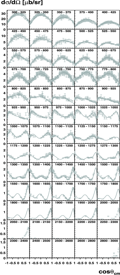
Figure 1: Differential cross sections $\rm d\sigma/d\Omega$ versus $\cos\Theta_{\rm cm}$ as measured by various experiments before CB-ELSA. The data stem from SAID . The SAID model for the respective energy interval is shown as solid line. The photon energy range in MeV is indicated in the subfigures.

In general, there is good coverage at lower energies. At beam energies above 2 GeV, there are only few data points measured by different experiments at discrete angles.

The description of the data using the SAID model is also shown in Fig. 1. The SAID model was fitted to these data points and thus, is only reliable up to an incoming photon energy of about 2 GeV.

In the following, a summary of the experiments performed and published after 1979 is given.

Yoshioka et al. Yoshioka:1980vu extracted differential cross sections for photon-beam energies between 390 and 975 MeV in energy bins of 20 to 25 MeV. They measured at 11 scattering angles covering a range in the center-of-mass system (cms) of $15^{\circ}<\Theta_{\rm cm}<130^{\circ}$ corresponding to $-0.64<\cos\Theta_{\rm cm}<0.97$.

At the Saskatchewan Accelerator Laboratory, differential cross sections were measured for 11 energies within 25 MeV above the $\pi^{0}$-photoproduction threshold Bergstrom:1997jc . The Igloo spectrometer was used, which was especially designed for an excellent $\pi^{0}$-detection efficiency. A full angular coverage from $0^{\circ}$ to $180^{\circ}$ was achieved.

Beck et al. measured differential cross sections at the electron accelerator MAMI for five energy bins from threshold at 144 MeV up to photon-beam energies of 157 MeV Beck:1990da and for six further bins between 270 MeV and 420 MeV Beck:1997ew . Both experiments used a linearly-polarized photon beam produced via coherent bremsstrahlung. In Beck:1997ew , the reaction was studied with the DAPHNE detector which covers $\sim$ 94 % of the solid angle.

Differential and total cross sections were determined with TAPS at MAMI Fuchs:1996ja . The TAPS collaboration measured at nine different energies between threshold and 280 MeV. The setup used five blocks of crystals resulting in coverage of the full angular range in $\Theta_{\rm cm}$, but only in partial coverage of the azimuthal angle. The experiment covered about 50% of the total solid angle. The published data are restricted to energies below 152.5 MeV. The contribution of the $E_{0+}$ multipole was extracted and compared to predictions from chiral perturbation theory and low-energy theorems.

Krusche et al. Krusche:1999tv extended the experiment to cover the energy range up to 792 MeV, which was the maximum possible energy at MAMI. A comparison was made between $\pi^{0}$ photoproduction off protons and off deuterons.

Schmidt et al. Schmidt:2001vg measured differential and total cross sections for $\pi^{0}$ photoproduction for incoming photon energies between threshold and 165 MeV. The measured data points were then also compared to predictions based on chiral perturbation theory and low-energy theorems.

Ahrens et al. Ahrens:2002gu measured differential cross sections for 12 energies in the photon-energy range between 550 and 790 MeV using the DAPHNE detector at MAMI. The availability of a polarized photon beam and a polarized target made it possible to measure the helicity difference $\sigma_{3/2}-\sigma_{1/2}$. The goal of the experiment was to test the GDH sum rule Gerasimov:1965et .

At BNL, photoproduction cross sections for $\pi^{0}$ mesons were measured using LEGS. Final-state particles were detected in an array of six NaI crystals. The data cover the beam-energy range from 213 MeV to 333 MeV. Unpolarized differential cross sections as well as beam asymmetries were determined Blanpied:2001ae .

This compilation shows that (almost) all data taken after 1979 cover only the lower photon-beam energy range up to 1 GeV. Data above 1 GeV stem from even older experiments; they are included in the SAID database SAID , too. The only recent publications comprising new experimental data on $\pi^{0}$ photoproduction originate from the GRAAL Collaboration Bartalini:2005wx and from this experiment Bartholomy:2004uz .

All available data (except Bartholomy:2004uz ; Bartalini:2005wx ) were reproduced well by the SAID model solution SM02 SAID . Data and fit results are shown in Fig. 1. The partial-wave analysis (PWA) also included $\pi$N-scattering data and determined masses, widths, and photocouplings of baryon resonances. The fit covered a photon-energy range up to 2 GeV. Contributions of the following resonances were extracted Arndt:2002 :
N(1440)P₁₁, N(1520)D₁₃, N(1535)S₁₁, N(1650)S₁₁,
N(1675)D₁₅, N(1680)F₁₅, $\Delta$(1232)P₃₃, $\Delta$(1620)S₃₁,
$\Delta$(1700)D₃₃, $\Delta$(1905)F₃₅, $\Delta$(1930) D₃₅, and $\Delta$(1950)F₃₇.
Recently, a new SAID model solution (SM05) has been released which, in addition, takes into account the data presented in this paper, our data on $\rm\gamma p\to p\eta$ Crede:2003ax and the new GRAAL data on $\rm\gamma p\rightarrow p\pi^{0}$ Bartalini:2005wx .

The Mainz unitary isobar model MAID concentrates on the photon-beam energy range below 1 GeV Drechsel:1999 . Extensions of MAID are in preparation Tiator:Trieste . Besides SAID and MAID there is a large number of other approaches to describe photon- and pion-induced production of mesons; a survey is given in the recent paper by Matsuyama, Sato and Lee Matsuyama:2006rp .

3 Experimental Setup

3.1 Overview

The CB-ELSA experiment was performed at the electron stretcher accelerator ELSA. The maximum achievable electron energy is 3.5 GeV.

The accelerator complex comprises three stages. A linear accelerator (LINAC) pre-accelerates electrons emitted by a thermionic electron gun to an energy of 20 MeV. These are transferred to a booster synchrotron, where they can be accelerated up to 1.6 GeV forming a pulsed beam ($f=50$ Hz). The electron bunches are injected into the stretcher ring over several cycles. The stretcher ring accumulates these bunches and accelerates the electrons up to the required energy. The electrons are made available for the CB-ELSA experiment via slow resonance extraction, with a duty factor of nearly 90%.

Figure 2: Experimental setup CB-ELSA, Bonn. The electron beam enters from the left side, hits the radiator, and produces bremsstrahlung. The photons are energy tagged and hit an LH₂ target in the center of the Crystal Barrel. Charged particles leaving the target are identified in the inner scintillating-fiber detector, photons are detected in the CsI(Tl) calorimeter. A photon counter for the flux determination is placed further downstream and is not shown in the figure.

The experimental setup is shown in Fig. 2. A first short overview of the different detector components is given below, which are then discussed in more detail in the following subsections.

The electrons hit a radiator target, where they produce bremsstrahlung. The energy of the photons, in the range between 25 % and 95 % of the primary electron energy, was determined via the detection of the corresponding scattered electrons in the tagging system. The primary electron beam of unscattered electrons was stopped in a beam dump situated upstream of the Crystal Barrel. The photon beam hit the liquid hydrogen (LH₂) target (length: $l=52.84$ mm, diameter: $d=30$ mm) placed in the center of the Crystal-Barrel detector.

The Crystal-Barrel detector forms the central component of the experiment. It consists of 1380 CsI(Tl) crystals and has an excellent photon-detection efficiency. The large solid-angle coverage and the high granularity allow for the reconstruction of multi-photon final states. A more detailed description of the Crystal-Barrel detector can be found in Aker:1992ny .

Charged particles leaving the target cannot be unambiguously identified by their energy depositions in the calorimeter. They were detected in a three-layer scintillating fiber detector surrounding the target Suft:2005inner . The first-level trigger of the experiment exploited detection of protons; it was provided by the tagging system in coincidence with the fiber detector. For the photon-senstitive second-level trigger a FAst Cluster Encoder (FACE), based on cellular logic, provided the number of clusters in the Crystal Barrel. A segmented total-absorption oil $\check{\rm C}$erenkov counter (not shown in Fig. 2) was placed further downstream to determine the total photon flux traversing the target.

3.2 Tagging System and $\gamma$-Counter

The photon beam was produced by bremsstrahlung off an amorphous copper foil of 3/1000 radiation length thickness. The total rate in the tagging system during the beamtime was 1-3$\cdot 10^{6}$ Hz. The unscattered electron beam, deflected by 7^∘, was annihilated in a beam dump consisting of heterogeneous materials including lead, boron-carbide, and polyethylene.

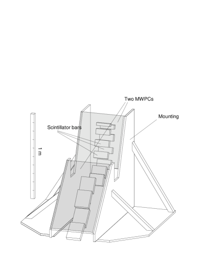
Figure 3: Layout of the tagging detector: The ladder of 14 scintillation bars and two proportional wire chambers are shown.

The tagging system is shown in Fig. 3. It serves to analyse the electron momentum spectrum behind the radiator. According to their energy loss, electrons are deflected in the dipole field of the tagging spectrometer; the field strength (1 - 2 T) was set according to the chosen beam energy. Assuming single photon radiation, the photon energy $E_{\gamma}$ is given by the beam energy $E_{\rm e,~{}ELSA}$ and the energy of the detected electron $E_{\rm e}^{\prime}$,

$$E_{\gamma}\,=\,E_{\rm e,~{}ELSA}\,-\,E_{\rm e}^{\prime}.$$ (2)

Tagged photons are assigned to hadronic events in the Crystal-Barrel setup by coincidences. Thus, the tagging system consists of two distinct parts, a 4 cm thick scintillator array to provide fast timing information, and two MWPCs with a total of 352 channels (with four channels overlap). Their spatial resolution translates into an energy interval per channel of 0.1 (0.5) MeV at the highest $E_{\gamma}$ and 10 (30) MeV at the lowest $E_{\gamma}$ for the beam energies of 1.4 (3.2) GeV, respectively, which were used for our measurements. The scintillator array was read out via photomultipliers. A logical OR of the left-right coincidences from all scintillators was required in the first-level trigger.

The tagging system was calibrated by direct injection of a very low intensity $e^{-}$-beam of 600 MeV or 800 MeV, after removing the radiator. Variation of the magnetic field of the tagging dipole enabled a scan of several spatial positions over the MWPCs. For a given wire, electron momentum and magnetic field strength are proportional. As long as saturation effects can be ignored, the magnetic current is proportional to the field.

The calibration was checked by Monte-Carlo trace simulations of the electron trajectories through the tagging magnet. Geometry of the setup, dimensions of the electron beam, angular divergences, multiple scattering and M$\o$ller scattering in the radiator foil and the air were taken into account. From these simulations, the energy of each of the MWPC wires was obtained by a polynomial fit. The uncertainty of the simulation was estimated to be of the same order of magnitude as the energy width of the respective wire. Deviations between the 600 MeV/800 MeV calibration could be attributed to effects of magnetic field saturation. Hence, the calibration of the highest photon energy points relied on an extrapolation of the simulated trajectories.

The hit-wire distribution of the MWPCs was measured with a minimum-bias trigger at a fixed rate of 1 Hz. This trigger required only a hit in the tagging system and was thus independent of hadronic cross sections. Accepted wire hits had to be isolated (one hit or cluster of hits); the small background was estimated from the time distribution of the associated tagger scintillator.

The absolute normalization was treated as a free parameter which was determined by fitting the measured angular distributions to the SAID cross sections. For the low-energy data ($E_{\rm e,~{}ELSA}=1.4$ GeV), the normalization constant was determined for each energy bin, and an error of $\pm 5\%$ was assigned to it. The $E_{\rm e,~{}ELSA}=3.2$-GeV data cover a region for which no SAID prediction is available. An energy-independent normalization constant was determined from a comparison of our differential cross sections with SAID for $0.8\leq E_{\gamma}\leq 1.7$ GeV. A systematic error of $\pm 15$% is estimated to account for possible variations of the background across the tagger.

Downstream of the tagger and behind the Crystal-Barrel detector a total absorption oil $\check{\rm C}$erenkov photon counter was mounted. It consists of three segments, each made of a hollow lead cylinder with 10 lead blades surrounded by mineral oil. The light produced by traversing particles was detected by two photomultipliers per segment.

3.3 Liquid H₂ Target

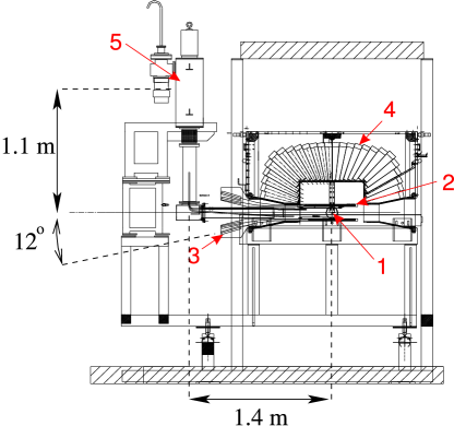
Figure 4: The liquid hydrogen target with target cell (1), inner SciFi detector (2) and photomultiplier readout (3) are situated in the center of the Crystal-Barrel calorimeter (4). Due to the geometry, there is a large distance between liquefier (5) and target.

Fig. 4 shows a side view of the assembly, the gas liquefier, one half of the Crystal-Barrel calorimeter, target cell, and inner scintillation fiber detector. The target cell cylinder is made of 125 $\mu$m Kapton foil; entrance and exit window have a thickness of 80 $\mu$m. The massive cold head of the H₂ refrigerator was mounted 2.5 m outside of the detector to avoid obstruction of the detector acceptance.

The Air Products (model CSA-208-L) refrigerator consists of a two-stage cooler head operating in a closed helium circuit according to the Gifford-McMahon principle. In the first stage, H₂ is liquefied. The second circuit consists of a large H₂ cold gas reservoir and the target cell connected via two Kapton pipes of 75 $\mu$m foil thickness serving as liquid H₂ supply and gaseous H₂ removal pipes.

3.4 Crystal Barrel

The Crystal-Barrel calorimeter is designed to provide high-efficiency photon detection with good energy and spatial resolution over an energy range from 20 MeV to 2 GeV. All crystal modules are arranged in a vertex-pointing geometry forming the shape of a barrel. The Crystal Barrel consists of 1380 CsI(Tl) crystals with a length of 30 cm corresponding to 16 radiation lengths and covering almost the complete solid angle. Each of the crystals is wrapped with a 0.1 mm titanium foil for mechanical stability and protection and a 2 mm support foil at the end (see Fig 6).

Fig. 6 shows a schematic diagram of the crystal arrangement. The special shape of the calorimeter requires 13 different types of crystals. They are arranged in 26 rings. Each ring has either 60 or 30 crystals, i.e. a single crystal covers $6^{\circ}$ (rings 1-10) or $12^{\circ}$ (rings 11-13) in azimuthal angle $\Phi$. In polar angle, a range from 12^∘ to 168^∘ is covered corresponding to a solid angle of 97.8% of 4$\pi$.

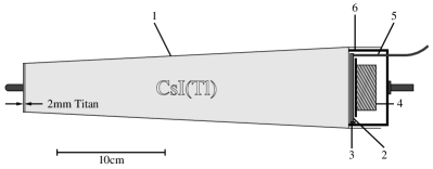
Figure 5: A crystal module: titanium case (1), wavelength shifter (2), photo-diode (3), preamplifier (4), optic fiber (5), case cover (6).

Figure 6: Mounting scheme of the Crystal-Barrel calorimeter. The numbers indicate the different crystal shapes.

The size of the crystal segments was adjusted to the Molière radius of CsI crystals, $r_{\rm M}=3.5$ cm. The 12^∘ opening on either side of the barrel is necessary for technical reasons. The segmentation limits the spatial resolution to 20 mrad ($\approx 1.1^{\circ}$) in $\Phi$ and $\Theta$. However, it allows the separation of two photons stemming from the decay of a $\pi^{0}$ meson with a maximum momentum of 1 GeV/$c$ corresponding to a minimum opening angle of 16.6^∘. The energy resolution of the calorimeter is empirically described by

$$\frac{\sigma_{E}}{E}\;=\;\frac{2.5\%}{\sqrt[4]{E\,[{\rm GeV}]}}\,.$$ (3)

For the readout of the scintillation light, silicon photodiodes are used. They are placed on a wavelength shifter (WLS) mounted on the rear end of the crystals and fulfilled two purposes. The WLS collect the light from the crystals over their full cross sectional area and transform the wavelength of the detected light to the sensitive range of the photodiode. CsI crystals emit light at wavelengths between 450 and 610 nm, with a maximum at 550 nm. The absorption profile of the WLS exhibits a maximum between 520 and 590 nm matching the range of emission of CsI. The light emitted by the WLS has a wavelength of 600 to 700 nm. For this wavelength, the WLS is practically transparent and the photodiode is most sensitive.

Preamplifiers are attached to the photodiodes on the crystal module to reduce the background noise. The overall gain stability of the CsI crystals is monitored by a light pulser system. For this purpose each WLS is connected via an optical fiber to a common Xenon flashlamp operating at a repetition rate of 5 Hz. The light is read out by the normal calorimeter electronics. Thus, crystal modules not working properly can easily be identified. In addition, the light pulser system is used to calibrate the high and the low range of the 12bit-dual range ADCs.

The Crystal Barrel was already used successfully for seven years at CERN (LEAR) before it was brought to Bonn. Changes of the photon yield in the crystals due to radiation damage were not observed. A detailed description of the CERN detector can be found in Aker:1992ny .

The calibration of the Crystal Barrel was carried out after data taking. For each crystal, the $\pi^{0}$ peak in the two-photon invariant mass was normalized iteratively to the nominal mass of $m_{\pi^{0}}=134.98$ MeV by taking the invariant masses of each pair of two photons. The mass resolution is $\sigma=8$ MeV at $m_{\pi^{0}}$ and $\sigma=15$ MeV at $m_{\eta}$ in their $2\gamma$ decays, and $\sigma=20$ MeV at $m_{\omega}$ (in its $\pi^{0}\gamma$ decay).

3.5 Inner Scintillating-Fiber Detector

The three-layer scintillating fiber detector identifies charged particles leaving the target and determines their intersection point with the detector Suft:2005inner . The 40 cm long detector is mounted on a 1.8 mm thick aluminum support structure. The fibers are 2 mm in diameter; they are positioned at mean radii of 5.81 cm, 6.17 cm and 6.45 cm, respectively. The innermost layer corresponds to a solid angle of 92.6% of 4$\pi$, thus covering almost the full solid angle of the barrel detector. The fibers of the outer layer were installed parallel to the z-axis, the fibers of the inner layer are bent clockwise, the remaining fibers are bent anti-clockwise, forming respectively, an angle of $-24.5^{\circ}$ or 25.7^∘ with the z-axis. Between each pair of layers, carbon cylinders hold the fibers in place. In total, the detector consists of 513 scintillating fibers read out via 16-channel-photomultipliers. Each scintillating fiber is coupled individually to an optical fiber guiding the signal through the backward opening of the barrel to the photomultipliers. The 3 layers had efficiencies of $94.8\pm 0.9$% (inner), $92.9\pm 0.9$% (middle), and $88.1\pm 0.8$% (outer), respectively. These values include the geometrical acceptance. The probability of two out of three layers having fired was $98.4\pm 0.2$% Suft:2005inner .

3.6 Trigger and Data Acquisition System

The first-level trigger demanded a coincidence of a hit in one of the tagger scintillators (related to an incoming photon) and of hits in two or three different layers of the inner scintillating-fiber detector (interpreted as detection of a proton in the final state). The tagger rate was of the order of 1-3$\cdot 10^{6}$ Hz; the coincidence with scintillating-fiber hits reduced this rate to 2000 Hz. The second level trigger defined the number of contiguous clusters of hit crystals. It used a fast cluster encoder (FACE) based on cellular logic. The decision time depended strongly on the complexity of the hit distribution in the Crystal Barrel and was typically 4 $\mu$s. In case of rejection of the event, a fast reset was generated, which cleared the readout electronics in 5 $\mu$s. Otherwise the readout of the full event was initiated; typical readout times were 5-10 ms. Along with an incoming trigger rate of 2000 Hz from the inner detector, this led to a dead time of 70% when two clusters were required by FACE. For three clusters in FACE, the dead time was negligible.

For the data presented here, events were only recorded if they had more than two clusters determined by FACE from the pattern of hit crystals. For part of the data the minimum number of clusters was set to three. The average overall data taking rate of the DAQ was 100 Hz or more, depending on whether empty channels were suppressed or not.

4 Data Analysis

The data presented here were taken from December 2000 until July 2001 in two run periods with different primary electron energies of 1.4 and 3.2 GeV. In the following, we refer to these data sets according to their incident electron energies. Cross sections were determined separately for the two different settings providing a total range of photon energies from 0.3 to 3 GeV. This corresponds to a range of $\gamma$p or p$\pi^{0}$ invariant masses from 1.2 to 2.6 GeV/$c^{2}$. The $\pi^{0}$ is reconstructed from its $\pi^{0}\to\gamma\gamma$ decay.

4.1 Photon Reconstruction in the Crystal Barrel

An electromagnetic shower will, in general, extend over several crystals. Such an area of contiguous calorimeter modules is called a “cluster”. In order to reduce the contributions of noise to the cluster energy, only crystals with an energy deposit above a threshold of 1 MeV are considered in the cluster finding algorithm. Within a cluster, a search was made for local energy maxima with an energy deposition above a minimum value of 20 MeV ($E_{\rm CLS}$). A crystal containing a local maximum of energy is referred to as a central crystal. Any local maximum is interpreted as evidence that a (charged or neutral) particle has hit the Crystal Barrel. Its energy deposit in the Barrel is called PED (particle energy deposit). If a cluster contains only one local maximum, the sum over all crystal energies in the cluster was then assigned to the energy of the PED ($E_{\rm PED}$). The center of gravity $\vec{x}=(\Theta,\Phi)$ of the energy distribution defines the spatial coordinates of the impact point on the Crystal-Barrel surface, and the momentum of a photon:

$$\vec{x}=\frac{\sum_{j}\left(P+\ln\left(\frac{E_{j}}{E_{\text{PED}}}\right)\right)\vec{x}_{j}}{\sum_{j}\left(P+\ln\frac{E_{j}}{E_{\text{PED}}}\right)}\quad$$ (4)

$$\text{ for }\quad\frac{E_{j}}{E_{\text{PED}}}\geq e^{-P}\,,$$ (5)

where $j$ runs over all crystals in the cluster and the cut-off parameter is $P=4.25$. A logarithmic weight has a stronger impact from small (and more distant) energy contributions leading to a better reconstruction accuracy of the photon direction. The weighting procedure was optimized performing extensive Monte-Carlo simulations. The PED is identified with a photon if it cannot be associated in space with the projection of a charged track (see below) extrapolated to the surface of the Crystal Barrel. Otherwise, it is identified as charged particle and here, by default, as proton.

If more than one local energy maximum is found inside a cluster, the energy of PED $i$ is determined from the energy deposit of the central crystals and the deposits of the up to eight neighbors, summed up to form $E_{9}^{i}$. The total energy of the cluster is then shared between the PEDs $j=1,2,\cdots$ according to the relative magnitude of their $E_{9}$-sums:

$$E^{i}_{\mbox{PED}}\;=\;\frac{E_{9}^{i}}{\sum_{j}E_{9}^{j}}\;E_{\mbox{cluster}}\quad{\mbox{and}}\quad E_{9}\;=\;\sum_{i=k}^{9}\;E_{k}\;,$$ (6)

where crystal energies in overlapping regions are split according to the relative energy deposits of the local maxima.

Monte Carlo simulations showed that the reconstructed photon energies differ from the initial values due to energy loss in insensitive parts of the detector. A PED-energy- and $\Theta$-dependent function derived from MC simulations was applied to the reconstructed energies.

Statistical shower fluctuations can generate additional maxima which are called split-offs and may be misidentified as photons. A single photon can create several split-offs, so that some good events are not considered in the analysis due to a wrong PED multiplicity in the barrel. About 5% of all photon showers create such split-offs. Split-offs can also be generated by charged particles, e.g. by nuclear reactions. The Monte Carlo simulation reproduces split-offs rather precisely. The error originating from split-offs is estimated to be less than 2% Amsler:1993kg .

4.2 Identification of Charged Particles

The event reconstruction in the Crystal Barrel provides direction and energy of a photon ($\Phi,~{}\Theta$, and $E~{}+$ with errors). High-energy charged particles like protons and pions can traverse the whole length of a crystal module without depositing all their kinetic energy in the CsI crystals. Pions originating in the target center and traversing the Crystal Barrel show a minimum ionizing peak at about 170 MeV. Their kinetic energy cannot be deduced from their energy deposit in the Crystal Barrel. The energy deposit of protons is larger and reaches a maximum for those stopping at the rear end of the Crystals. Protons stopping earlier and penetrating protons deposit less energy. A given PED energy of a proton corresponds therefore to two allowed values for the proton kinetic energy. In this analysis, the proton PED energy was not used.

Identification of charged PEDs was important to perform the analysis even though proton PEDs were ignored after identification. Charged particles produce usually single-crystal clusters, and the reconstructed angles $\Theta$ and $\Phi$ agree in most cases with a crystal center, leading to regular spikes in the proton angular distribution. Therefore, protons were treated as missing particles in a kinematic fit.

A charged particle traversing the fiber detector can fire one or two adjacent fibers in each layer forming a British-flag-like pattern which defines the impact point (see Fig. 7, left). A single charged particle may also fake three intersection points (see Fig. 7, middle). In order not to loose these events, up to three intersection points were accepted in the reconstruction. One inefficiency (one broken or missing fiber) leading to a pattern shown in Fig. 7, right, was accepted by the reconstruction routines.

The accuracy of the reconstruction of the impact point was studied using simulations and was determined to $\pm 0.5$ mm in the x- and y- coordinates (representing the resolution in $\Phi$). The error in the z coordinate was determined to be 1.6 mm. Trajectories were formed from the center of the hydrogen target to the impact point in the fiber detector as well as to all PEDs in the barrel. For all resulting combinations, the angle between the trajectories was calculated. A PED in the Crystal Barrel was identified as a charged particle if the angle between a trajectory starting in the target center and hitting the fiber impact point and the trajectory from target center to the Crystal-Barrel PED was smaller than $\approx 20^{\circ}(\,=0.35~{}{\rm rad})$. This procedure is called matching.

Figure 7: Charged particles crossing the inner fiber detector produce different hit patterns. A hit in three layers may result in one unique intersection point or in three intersection points (middle). One inefficiency still yields a defined intersection point (right).

In some cases, there was more than one hit per layer. If the hits belonged to adjacent fibers, the clusters were assigned to the central fiber (two wires give an effective fiber number $(2n+1)/2$); otherwise, more than one impact point was reconstructed. Each impact point was tested if it can be matched to a PED in the Crystal Barrel. Matched PEDs are identified as protons. Only one proton is allowed in the event reconstruction. Events with two matched PEDs, possibly due to $\rm p\pi^{+}\pi^{-}\pi^{0}$ with one undetected charged particle, were rejected.

Protons going backwards in the center-of-mass system have rather low momenta. The minimum momentum for a proton to traverse the target cell, wrappings, inner detector, and Crystal-Barrel support structure and to deposit 20 MeV in a crystal is 420 MeV/$c$. To reconstruct events with protons having smaller momenta, events with two PEDs in the Crystal Barrel were taken into account when they had a hit in the inner detector not matching one of the two PEDs. It was then assumed that the two PEDs were photons and that the proton got stuck in the inner detector or support structure between scintillation fiber detector and the barrel. Thus, proton momenta down to 260 MeV/$c$ were also accessible in the analysis.

4.3 Event Reconstruction

In the first step of data reduction, both photons from a $\pi^{0}$ decay were required to be detected in the Crystal Barrel, irrespective of the detection of the proton. Thus, events with 2 or 3 PEDs in the Crystal Barrel were selected. If a proton candidate was found in the fiber detector, and the fiber hit could be matched to a barrel hit, the corresponding PED was identified as proton and excluded from further analysis. The proton was thus treated as missing particle. Unmatched PEDs were considered to be photons. All events with two photons were kept for further analysis. In this way, consistency between the two data sets (with and without observed proton) was guaranteed.

In total, $\sim$45 million events were assigned to these two event classes and subsequently subjected to a kinematic fit as described in the following.

Kinematic fits minimize the deviation of measured quantities from constraints like energy and momentum conservation. The measured values $y_{i}$ are varied (by $\delta y_{i}$) within the estimated errors $\sigma_{i}$ until the constraints are fulfilled exactly. Further constraints are given by the known masses of particles like $\pi^{0}$ or $\eta$ which are reconstructed from the 4-momenta of photons. Kinematic fitting improves the accuracy by returning corrected quantities, which fulfill the constraints exactly. A $\chi^{2}$ value can be calculated from the minimization given by

$$\chi^{2}\;=\;\sum_{i}\>\left(\frac{\delta y_{i}}{\sigma_{i}}\right)^{2}\;.$$ (7)

In our experiment, the quantities $y_{i}$ are the measured values $(\Phi,\Theta,\sqrt{E})$. Since a fraction of the energy can be lost (but never created) in some material, the distribution of $E$ is asymmetric; therefore $\sqrt{E}$ is chosen as variable which exhibits a more Gaussian distribution than $E$.

If the $y_{i}$ measurement errors are correlated, then this becomes a matrix equation. Each constraint equation is linearized and added, via the Lagrange multiplier technique, to the $\chi^{2}$ equation:

$$\chi^{2}\;=\;(\delta\vec{y}\,)^{T}{\bf V}^{-1}(\delta\vec{y}\,)\>+\>2\vec{a}\,^{T}\vec{f}(\vec{y}+\delta\vec{y}\,)\;,$$ (8)

where ${\bf V}$ is the covariance matrix for the measurements $\vec{y}=(y_{i})$; $\vec{a}$ is the vector of Lagrange multipliers for the constraints $\vec{f}$, and $\delta\vec{y}$ denote the required variations. When the constraining equations are satisfied and the experimental error matrix correctly determined, then the difference between true values $y_{i}$ and the measurements $y_{i}+\delta y_{i}$ should be of the same magnitude as the errors. If the data are distributed according to a Gaussian function, a probability distribution for the $\chi^{2}$ with $n$ degrees of freedom can be defined by

$$P(\chi^{2};n)\;=\;\frac{2^{-n/2}}{\Gamma(n/2)}\>\chi^{n-2}\>{\mbox{e}}^{-\chi^{2}/2}\;,$$ (9)

which is called the $\chi^{2}$ probability. To make judgments and decisions about the quality of the fit, the relevant quantity is the integral

$$CL(\chi^{2})\;=\;\int_{\chi^{2}}^{\infty}P(\chi^{2};n)\>d\chi^{2}\;,$$ (10)

which is called the confidence level. The $\chi^{2}$ calculation depends directly on the errors of the measured values. In this case, the errors are the measurement errors of the calorimeter hits: the polar angle $\Theta$, the azimuthal angle $\Phi$ and the energy $E$ of a calorimeter cluster. If the errors and, hence, the covariance matrix are correctly determined, the confidence level distribution of the fits should be flat. A sharp rise near zero of the confidence level distribution can indicate contributions from background events. The kinematical fit is thus an ideal method to quantify the quality of different final-state hypotheses for an event.

Figure 8: Deviations between the measured values $\Phi$ (a), $\Theta$ (b), $\sqrt{E}$ (c) and $E_{\gamma}$ (d) as the results from a kinematic fit in units of the respective measurement errors (1.4 GeV data). After calibration, the mean values should be 0 and the variance 1. The experimental distributions are compatible with these numbers.

A pull is a measure of the displacement of the measured values to the fitted values normalized to the corresponding errors. The measured values $y_{i}$ with errors $\sigma_{i}$ are corrected by shifts $\delta y_{i}$ leading to new values $y_{i}+\delta y_{i}$ which fulfill exactly the constraints and have smaller errors ${\sigma^{\prime}}_{i}$. The quantity

$${\rm pull_{i}}=\frac{\delta y_{i}}{\sqrt{\sigma_{i}^{2}-{\sigma^{\prime}}_{i}^{2}}}$$ (11)

is called pull; it should be Gaussian with unit width and centered around zero. Fig. 8 shows the pulls for the Crystal Barrel quantities ($\Phi$, $\Theta$, $\sqrt{E}$) and the photon beam energy $E_{\gamma}$. Mean values are all compatible with zero, the variances are close to (but slightly above) 1.

A systematic offset in a measured quantity will move the center of its pull distribution away from zero. Using this information in addition to kinematic fits treating the z vertex as free parameter, an (unwanted) target displacement of 0.65 cm from the central position towards the tagging system was detected, in perfect agreement with a later position measurement.

In a preselection, the compatibility of events with the hypothesis

$$\rm\gamma p\rightarrow p2\gamma$$ (12)

was tested in a one-constraint (1C) kinematic fit imposing energy and momentum conservation but leaving the proton 3-momentum as adjustable quantity. The confidence level distribution of the fit is shown in Fig. 9. Above 20%, the confidence level distribution is

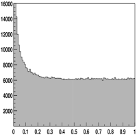
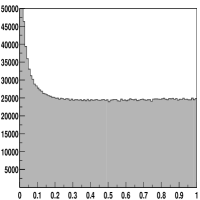
Figure 9: Confidence level distributions (number of events as a function of CL) for the one-constraint kinematic fit to the hypothesis $\rm\gamma p\rightarrow p2\gamma$ imposing energy and momentum conservation and treating the proton as unseen particle for 1.4-GeV data (left) and the corresponding Monte Carlo simulations (right).

flat in both data and Monte Carlo events. At small confidence level CL, the distribution increases when CL approaches zero in both distributions. In the data, this could indicate the influence of background events or of too small errors for a subclass of events. In the Monte Carlo simulation shown in Fig. 9, only p$\pi^{0}$ events were created and no background events. Hence the events with small confidence level must be true p$\pi^{0}$ events. Indeed, inspection of $\gamma\gamma$ invariant mass distribution shows that these events are $\rm p\pi^{0}$ events with larger errors. The assumption made in the kinematic fit that the errors do not depend on the kinematics of the event is obviously wrong. A cut at e.g. 10% confidence level entails therefore the risk that events with larger errors, preferentially events with $\pi^{0}$ in forward direction, have only a small detection efficiency. This would lead to a loss of statistics and, in case of differences between data and simulations, to wrong results.

Here, a cut on the confidence level at $10^{-4}$ was applied. This cut rejects all events where the kinematic fit fails (CL=0) and very badly measured events. It was checked that the rejected events have a $\gamma\gamma$ mass distribution with very few $\pi^{0}$ only.

Fig. 10 shows $\gamma\gamma$ invariant mass spectra after the confidence level cut: (a) for the low-energy run and (b) for the high-energy run. There are approximately $2.44\cdot 10^{6}$ ($1.32\cdot 10^{6}$) $\pi^{0}$ events in the low-energy and $572\cdot 10^{3}$ ($144\cdot 10^{3}$) $\pi^{0}$ events in the high-energy data set. The numbers in parentheses give the number of events with a proton seen by the Crystal-Barrel detector. This fraction is larger for the high-energy run where the tagged energy range started at higher energy, and more protons escaped through the forward hole. For a fraction of this data, a more restrictive trigger excluded events with only 2 detected particles.

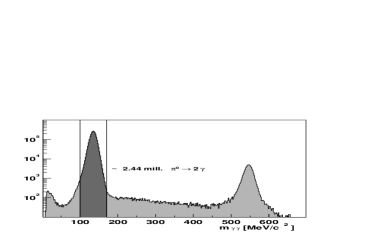
(a) 1.4 GeV data

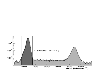
(b) 3.2 GeV data

Figure 10: Two-photon invariant mass spectra using events with two properly reconstructed photons. Note the logarithmic scale. A kinematic fit to the $\rm\gamma p\rightarrow p\gamma\gamma$ hypothesis was performed and a confidence level cut of $10^{-4}$ applied. The dark grey area, defined by an additional mass cut, corresponds to accepted events. The low-mass asymmetry of the $\pi^{0}$ peak is due to energy overflow in the ADCs for high-energetic photons. It is well reproduced by Monte Carlo simulations.

The $\pi^{0}$ meson is observed above an almost negligible background at a level of $10^{-3}$. The remaining background under the $\pi^{0}$ at high energies was subtracted using side bins, which contained typically a few events. Empty-target runs were used to determine additional background. After all cuts had been applied, very few events survived in empty-target runs. In LH₂ data, only $2\pm 2$ % were background events not stemming from LH₂.

Cuts in the invariant mass were applied in addition to the kinematic fits. The criterion for a $\pi^{0}$ meson was a $2\gamma$ mass in the ($135\pm$35) MeV/$c^{2}$ interval. At high photon energies, the cut was widened to the 75 – 175 MeV/$c^{2}$ region. For the low-energy run, a second kinematic fit was applied constraining the two-photon invariant mass to the $\pi^{0}$ mass (two-constraint fit).

4.4 Monte-Carlo Simulations

The detector was simulated by cb-geant, a Monte Carlo program based on the CERN program package geant3. The geometry of the barrel calorimeter was implemented accurately. Only the type-11 crystals (see fig. 6) had to be approximated since geant3 did not support their non-trapezoidal shape.

A number of small energy correction factors were applied to the simulated energy deposits in the CsI crystals. Photons of larger energy have a shower profile penetrating deeper into the crystals. The efficiency of light collection is higher by several per cent at the rear end of a crystal. In addition, the light collection efficiency is different for different crystal shapes. The mean energy loss due to shower leakage into support material was determined from the simulations. These effects required empirical corrections of the reconstructed photon energies.

(a) $\rm\gamma p\rightarrow p\pi^{0}$ ,1.4 GeV

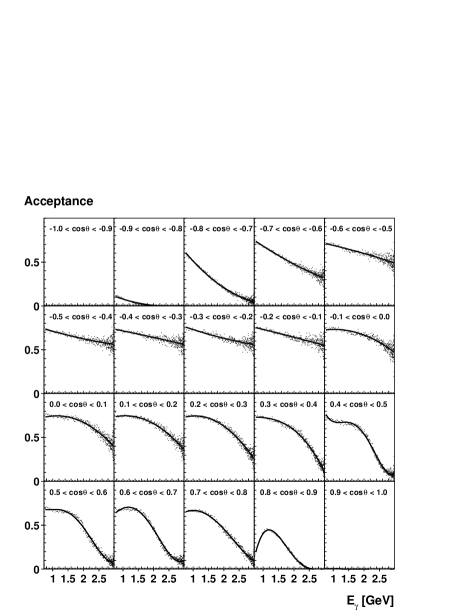
(b) $\rm\gamma p\rightarrow p\pi^{0}$ , 3.2 GeV

Figure 11: Acceptance as a function of tagger wire number for the 20 $\cos\Theta_{cms}$ bins from $[-1.0,0.9],\ldots,[0.9,1.0]$. The acceptances are plotted at the energy $E_{\gamma}$ of the corresponding wire. The acceptance is calculated using eq. (13). At large energies, the energy range covered by one wire is small, and the acceptances show statistical fluctuations due to limited Monte Carlo event numbers.

The fiber detector was implemented as a homogeneous cylindrical scintillation counter since simulating fibers with helix-shaped bending is not supported by geant3. Instead, the fiber number in each layer was calculated from the known impact point taking into account the real shape of the fibers. Single-fiber inefficiencies as derived from the data were taken into account to allow simulations of trigger efficiencies. The gaps between the cylinders were filled with a carbon-based support structure. The plastic-foil wrapping was simulated as described in (5.3.1).

The acceptance was determined from Monte-Carlo simulations as ratio of reconstructed and generated events:

$$A_{\pi^{0}\rightarrow 2\gamma}=\frac{N_{\rm rec,MC}}{N_{\rm gen,MC}}.$$ (13)

The acceptance is shown in Fig. 11 for the 20 $\cos\Theta_{\rm cm}$ bins and for both data sets as a function of the wire number. Instead of the wires number, the corresponding photon energy is plotted on the horizontal axis. $A_{\pi^{0}\rightarrow 2\gamma}$ reaches a maximum of 60% to 70% depending on the energy range. The acceptance is very small for $\cos\Theta_{\rm cm}>0.9$. The corresponding low-energetic protons hardly reach the fiber detector and thus the first-level trigger condition is not always met. For $\cos\Theta_{\rm cm}<-0.9$ (for backward $\pi^{0}$), protons simply escape through the forward hole not covered by the fiber detector. For high-energy $\pi^{0}$ mesons, the opening angle between the two decay photons is not large enough, and only a single PED is detected. Then the event is lost in the trigger and the detection efficiency is smaller at higher energies. To avoid biased results due to imperfections of the apparatus and/or the simulations, we required the detection efficiency to exceed a minimum of 5 %. For this reason, we rejected the last forward and backward data points.

5 Determination of Cross Sections

5.1 Basic Definitions

The unpolarized differential cross sections $\rm d\sigma/d\Omega$ can be calculated from the number of data events identified in the respective channel using

$$\frac{\rm d\sigma}{\rm d\Omega}=\frac{N_{{\rm\pi^{0}}\rightarrow 2\gamma}}{A_{{\rm\pi^{0}}\rightarrow 2\gamma}}\medspace\frac{1}{N_{\gamma}\rho_{\rm t}}\medspace\frac{1}{\Delta\Omega}\medspace\frac{\Gamma_{\rm total}}{\Gamma_{{\rm\pi^{0}}\rightarrow 2\gamma}},$$ (14)

where the quantities are:

$N_{\pi^{0}\rightarrow 2\gamma}$	: Number of events in ($E_{\gamma},\cos\Theta_{\rm cm}$) bin,
$A_{\pi^{0}\rightarrow 2\gamma}$	: Acceptance in ($E_{\gamma},\cos\Theta_{cm}$) bin,
$N_{\gamma}$	: Number of primary photons in $E$ bin,
$\rho_{\rm t}$	: Target area density,
$\Delta\Omega$	: Solid-angle interval $\Delta\Omega=2\pi\Delta(\cos\Theta_{\rm cm})$,
$\frac{\Gamma_{\pi^{0}\rightarrow 2\gamma}}{\Gamma_{\rm total}}$	: decay branching ratio.

The number of events in a $(E_{\gamma},\cos\Theta_{\rm cm})$ bin comprises events with two or three PEDs in which the proton was either undetected or detected in the Crystal Barrel. Summation of both contributions reduces the necessity of reproducing exactly the threshold behavior of low-energetic protons in the Crystal-Barrel detector. For part of the 3.2-GeV data run, three or more hits in the Crystal Barrel were already required by the hardware trigger (FACE). The most forward data point has thus a smaller number of events and a larger error.

The target area density is calculated from the density of liquid hydrogen $\rho({\rm LH}_{2})=0.0708\,$g/cm³ and its molar mass $M_{\rm mol}({\rm LH}_{2})=2.01588\,$g/mol to be

$$\rho_{\rm t}\ =\ \frac{2\rho({\rm LH}_{2})N_{\rm A}L}{M_{\rm mol}({\rm LH}_{2})}\ =\ 2.231\cdot 10^{-7}/\mu{\rm b},$$ (15)

where $N_{\rm A}=6.022\cdot 10^{23}\,$/mol is the Avogadro’s number, $l=52.75$ mm is the length of the active target cell, and the factor 2 accounts for the two atoms in ${\rm LH}_{2}$.

The $\pi^{0}$ was identified via its decay into $2\gamma$ which has a relative branching ratio of 98.798 %.

The solid-angle interval is

$$\Delta\Omega=2\pi\,\Delta(\cos\Theta_{\rm cm})\,,$$ (16)

where $\Delta(\cos\Theta_{\rm cm})=0.1$ gives the bin width of the angular distributions, subdividing $\cos\Theta_{\rm cm}$ into 20 bins. Photon-energy bins of about 25 MeV width were chosen for the 1.4 GeV data. The 3.2-GeV data are presented in bins of about 50 MeV, 100 MeV, and 200 MeV in the intervals $E_{\gamma}\in[750,2300],[2300,2600],[2600,3000]$, respectively.

5.2 Normalization

At $E_{\rm e,~{}ELSA}=1.4$ GeV, the SAID-SM02 model description of $\rm\gamma p\to p\pi^{0}$ was used for the absolute normalization of our measured angular distributions. We minimized the function

$$\sum_{i=0}^{n-1}\frac{(x\cdot N_{i}-S_{i})^{2}}{(\delta_{N_{i}})^{2}}$$ (17)

for each energy channel of the tagging system, where $i$ denotes a bin in $\cos\Theta_{\rm cm}$, $N_{i}$ are the acceptance-corrected number of data events, $\delta_{N_{i}}$ are the errors in $N_{i}$, and $S_{i}$ are the values of the SAID model integrated over the corresponding energy bins. Furthermore, $x$ stands for a normalization factor including all normalization constants of Eq. (14), it is used as free fit parameter. This method works well for the energy region between threshold and $E_{\gamma}\approx 2$ GeV, where the SAID model is reliable. The extracted photon flux leads also in the channel $\rm\gamma p\to p\eta$ to cross sections which are consistent with previous data. We estimate the error of the normalization to be $\pm 5$%. The error given by the statistical spread of all data on $\pi^{0}$ photoproduction used by SAID is not taken into account.

The method of normalizing to a known cross section was not applicable to our data at $E_{\rm e,~{}ELSA}=3.2$ GeV since our data extend the currently available world database substantially. Instead, we relied on the measured number of electrons in the tagger, which is proportional to the photon flux. A normalization factor was determined from a fit to SAID-SM02 in the energy range up to 1.7 GeV and applied to the full energy range. Some systematic deviations in the absolute cross section of the order of 10-15 % occur in the lowest bins, for 800 - 950 MeV. The deviations are not caused by uncertainties in detection efficiency. This follows from the perfect agreement of the $2\gamma$ and $3\pi^{0}$ decay channels of the $\eta$ in $\rm\gamma p\to p\eta$ Crede:2003ax . Thus, we believe that within a systematic error of 15 % we can trust this normalization, even above incoming photon energies of 2 GeV.

5.3 Systematic Uncertainties

Systematic errors were studied in Monte-Carlo simulations. The errors, with exception of the normalization error, were added quadratically for each point in the differential cross section. The total systematic error is then added quadratically to the statistical error. The systematic errors discussed in the following subsection are included in the shown error bars. The statistical errors are small, except for the most forward and most backward points in the angular distributions.

The following effects contribute to the systematic uncertainty of the measurements:

5.3.1 Reconstruction Efficiency

The reconstruction of neutral mesons and the identification of final states required a sequence of cuts including those on the results of kinematic fitting. An overall uncertainty of $\pm 5.7$% was assigned to the reconstruction efficiency as determined in Amsler:1993kg . This error includes uncertainties due to split-offs.

5.3.2 Target Position

The position of the target cell was determined by comparing results from kinematic fitting (off-zero displacement of pull distributions) to Monte-Carlo simulations. The target was found to be shifted upstream by 0.65 cm, i.e. into the direction of the tagger with respect to the center of the Crystal Barrel. The acceptances of the $\rm\gamma p\rightarrow p\pi^{0}$  reaction were re-determined for target shifts of $\pm 3$ mm compared to the real target position. The variations in the differential cross sections that resulted from these changes depend on energy and angle are as large as 5% for forward protons and $\pm 1$% on average.

5.3.3 Position of Beam Axis

The position of the photon beam measured by a beam profile monitor showed slight variations in time and even within an extraction cycle. Analyzing data from the inner detector, this shift was found to be less than 3 mm off axis at the target position. The acceptances were re-calculated assuming a shifted vertex distribution and the resulting cross section changes were included as systematic uncertainty. The errors due to beam shifts are, depending on energy and angle, 2% or smaller.

5.3.4 Material between Target and Crystal Barrel

All material between target and sensitive detector components was simulated carefully. However, black tape and foil was used to wrap the inner detector to get it light-tight; its thickness was not exactly known. Small changes in the thickness of this material had large effects on the resulting detection efficiency for low energy protons and on the trigger efficiency (which required at least two layers of the scintillation fiber detector to have fired). Assuming the worst case of 1 mm of additional or missing material, simulations were performed, new acceptances calculated and systematic uncertainties in the cross sections determined. This error was negligible.

5.3.5 Solid Angle

Events belonging to one bin in $\cos\Theta_{\rm cm}$ may be reconstructed in an adjacent bin. This migration effect was studied by unfolding the resolution in $\cos\Theta_{\rm cm}$ by Monte Carlo methods and found not to contribute significantly to the results.

5.3.6 Target Thickness

The target thickness does not contribute to the error since our cross sections are normalized to SAID.

5.3.7 Photon Flux

Our angular distributions are normalized to SAID, as outlined in section 5.2. We assign an error of $\pm 5$% ($\pm 15$%) to the normalization of the 1.4 GeV (3.2 GeV) data. These errors are not included in Figs. 12-14.

6 Experimental Results

Differential cross sections were calculated separately for the two different ELSA energies of 1.4 GeV and 3.2 GeV. The data sets published in Bartholomy:2004uz contained the complete 1.4-GeV data set covering the photon energy range from 0.8 to 1.3 GeV and the 1.3 to 3.0 GeV range from the 3.2-GeV data set.

6.1 Differential Cross Sections $\bf\rm d\sigma/d\Omega$ for $\boldsymbol{\gamma}\textbf{p}\boldsymbol{\rightarrow}\textbf{p}\boldsymbol{\pi}^{\textbf{0}}$  at an Electron-Beam Energy of 1.4 GeV

The differential cross sections are shown in Fig. 12 together with the SAID-SM02 model curve. Statistical and systematic errors are added quadratically. In general,

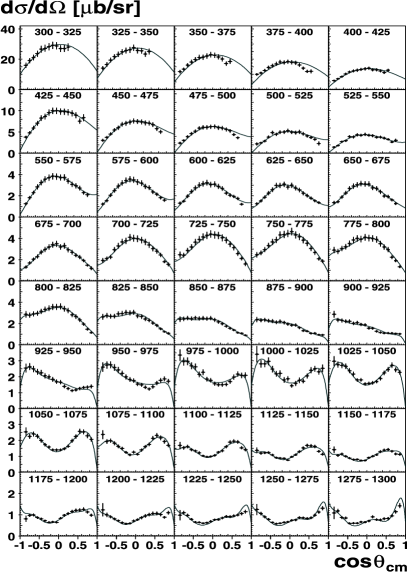
Figure 12: Differential cross sections for $\rm\gamma p\rightarrow p\pi^{0}$  from the low-energy data. Statistical and systematic errors are added quadratically. The photon flux was determined by normalizing the distributions to the SAID-SM02 model. The photon energy range (in MeV) is given in each subfigure. The symbols are: ◼: CB-ELSA, —: SAID-SM02.

the agreement is impressive. Note, however, that the data are normalized to SAID in each energy bin. At the lowest energies, we encounter some deviations from SAID. We cannot exclude systematic effects beyond those listed in section 5.3. They may be due to the rather small kinetic energies of the recoil protons from the reaction $\rm\gamma p\rightarrow p\pi^{0}$ , just at the threshold to trigger the inner detector. The high tagger rates in this energy region may also be responsible for the problems.

6.2 Differential Cross Sections $\bf\rm d\boldsymbol{\sigma}/d\boldsymbol{\Omega}$ for $\boldsymbol{\gamma}\textbf{p}\boldsymbol{\rightarrow}\textbf{p}\boldsymbol{\pi}^{\textbf{0}}$  at 3.2 GeV

Fig. 13 shows the angular distributions for the reaction $\rm\gamma p\rightarrow p\pi^{0}$  for the high-energy data set. SAID-SM02 results are shown for comparison. There is good overall agreement between data and SAID. At the smallest energies, the agreement is somewhat worse. For this data, one normalization factor is used.

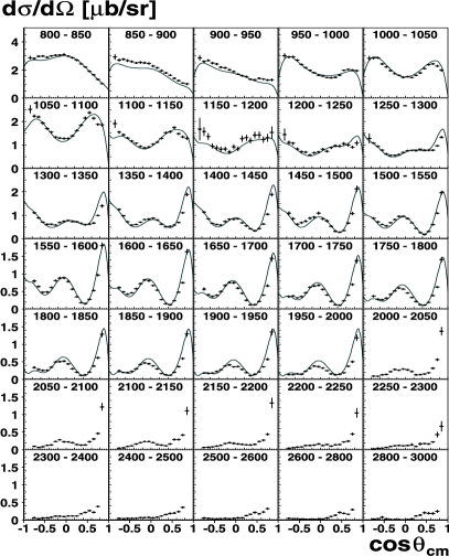
Figure 13: Differential cross sections for $\rm\gamma p\rightarrow p\pi^{0}$  from the high-energy data. Statistical and systematic errors are added quadratically. The absolute normalization was determined by fitting the angular distributions in the range from 800 MeV to 1.7 GeV to the SAID-SM02 model. The photon energy range (in MeV) is given in each subfigure. The SAID-SM02 model result is shown as solid line.

The two data sets are combined by using the 1.4-GeV data set up to the maximum possible photon energy of 1.3 GeV and using the 3.2 GeV data set to cover the range from 1.3 GeV to 3 GeV photon energy. We restrained from calculating mean values for $0.8\leq E_{\gamma}\leq 1.3$ GeV since the final errors are dominated by common systematic errors. For this energy region, we used the 1.4-GeV data because of the finer binning and since the tagger worked more reliably in the high energy part where the intensity is lower.

6.3 Differential Cross Sections $\rm d\sigma/d\Omega$ for $\boldsymbol{\gamma}\textbf{p}\boldsymbol{\rightarrow}\textbf{p}\boldsymbol{\pi}^{\textbf{0}}$ , Combined Data Set

The cross sections from threshold to 3 GeV are shown in Fig. 14. Data points are shown as open circles with error bars. The solid line represents a fit described below. The MAID results Drechsel:1999 for photon energies up to 1 GeV are given by dotted lines, results of the new SAID model SM05 for photon energies up to 2 GeV as dashed lines. The agreement between data and the models is equally good for both data sets. The angular distributions show rapid variations depending on both energy and emission angle of the meson, reflecting the contributions from many partial waves.

Figure 14: Previous page: Differential cross sections for $\rm\gamma p\rightarrow p\pi^{0}$ ; combined data set. Statistical and systematic errors are added quadratically. The solid line represents a fit to the partial waves described below, the dashed line is the SAID SM05, the dotted line the MAID model.

6.4 Partial Wave Analysis

The strong variations in the differential cross sections indicate strong contributions of various resonances with different quantum numbers. To determine quantum numbers and properties of contributing resonances, the differential $\rm\gamma p\to p\pi^{0}$ cross sections were used in a partial wave analysis. The analysis was based on an isobar model. In the $s$-channel, $\rm N^{*}$ and $\rm\Delta^{*}$ contribute to the $\rm p\pi^{0}$ final state. The background in this channel was described by reggeized $t$-channel $\rho$ ($\omega$) exchange and by baryon exchange in the $u$-channel. In addition $s$-channel Born-terms were included in the fits. Details on the partial wave analysis can be found in Anisovich:2004zz ; Anisovich:2005tf . The CB-ELSA data on $\rm\gamma p\to p\pi^{0}$ and $\rm\gamma p\to p\eta$ Bartholomy:2004uz ; Crede:2003ax were included as well as additional data sets from other experiments: Mainz-TAPS data Krusche:nv on $\eta$ photoproduction, beam-asymmetry measurements of $\pi^{0}$ and $\eta$ Bartalini:2005wx ; SAID1 ; SAID2 , and data on $\rm\gamma p\rightarrow n\pi^{+}$ GRAAL2 . The high precision data from GRAAL Bartalini:2005wx do not cover the low mass region; therefore we extracted further data from the compilation of the SAID database SAID1 . Data on photoproduction of $\rm K^{+}\Lambda$, $\rm K^{+}\Sigma^{0}$, and $\rm K^{0}\Sigma^{+}$ from SAPHIR Glander:2003jw ; Lawall:2005np and CLAS McNabb:2003nf , and beam asymmetry data for $\rm K^{+}\Lambda$, $\rm K^{+}\Sigma^{0}$ from LEPS Zegers:2003ux were also included in the analysis. This partial wave analysis is much better constrained than an analysis using the $\rm\gamma p\to p\pi^{0}$ data only. The main results on baryon resonances coupling to $\rm p\pi^{0}$ and $\rm p\eta$ are discussed in Anisovich:2005tf , those to $\rm K^{+}\Lambda$ and $\rm K^{+}\Sigma^{0}$ are documented in Sarantsev:2005tg .

To describe the different data sets, 14  N^∗ resonances coupling to N$\pi$, N$\eta$, $\rm K\Lambda$, and $\rm K\Sigma$ and 7 $\rm\Delta^{*}$ resonances coupling to N$\pi$ and $\rm K\Sigma$ were needed. Not all included resonances contribute to the $\rm p\pi^{0}$ final state. Most resonances were described by relativistic Breit-Wigner amplitudes. For the two S₁₁ resonances at 1535 and 1650 MeV, a four-channel $K$-matrix ($\rm N\pi$, $\rm N\eta$, $\rm K\Lambda$, $\rm K\Sigma$) was used.

The total cross section and the main results of the PWA are briefly discussed in the next section.

6.5 Total Cross Section and Results of the Partial Wave Analysis

From the differential cross sections, the total cross section was determined by integration. The integration was performed by summing over the differential cross sections of Fig. 14 and using extrapolated values from the fit for bins with no data. In the total cross section, shown in Fig. 15, clear peaks are observed for the first, second, and third resonance region. The fourth resonance region exhibits a broad enhancement at W about 1900 MeV. The decomposition of the peaks into partial waves and their physical significance will be discussed below.

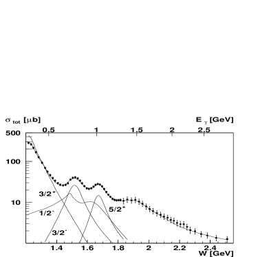
Figure 15: Total cross section (logarithmic scale) for the reaction $\rm\gamma p\rightarrow p\pi^{0}$ obtained by integration of angular distributions of the CB-ELSA data and extrapolation into forward and backward regions using our PWA result. The solid line represents the result of the PWA. Four individual contributions to the cross section are also shown.

The first resonance region is the dominant structure of Fig. 15. It is due to excitation of the $\rm\Delta(1232)P_{33}$. There is strong destructive interference between $\rm\Delta(1232)$ $\rm P_{33}$, the $\rm P_{33}$ nonresonant amplitude, and $u$-channel exchange. The $\rm N(1440)P_{11}$ Roper resonance provides only a small contribution of about 1–3% compared to the $\rm\Delta(1232){\rm P}_{33}$. In the second resonance region, the $\rm N(1520)D_{13}$ and $\rm N(1535)S_{11}$ resonances yield contributions which are shown as thin lines in Fig. 15.

The third bump in the total cross section is due to three major contributions: the $\rm\Delta(1700)D_{33}$ resonance provides the largest fraction ($\sim\!35$%) of the peak, followed by $\rm N(1680)F_{15}$ ($\sim\!25$%) and $\rm N(1650)S_{11}$ ($\sim\!20$%). In addition the $\rm\Delta(1620)S_{31}$ ($\sim\!7$%) and $\rm N(1720)P_{13}$ ($\sim\!6$%) resonances are required. In the fourth resonance region, the $\rm\Delta(1950)F_{37}$ contributes $\sim\!41$% to the enhancement and $\rm\Delta(1920)P_{33}$ is identified with $\sim\!35$%. Additionally, the fit requires the presence of $\rm\Delta(1905)F_{35}$ and $\rm\Delta(1940)D_{33}$. The high-energy region is dominated by $\rho$($\omega$) exchange in the $t$-channel as can be seen by the forward peaking in the differential cross sections.

6.6 Differential Cross Sections $\bf d\sigma/dt$

The partial wave analysis assigns a fraction of the total cross section to $t$-channel exchange which increases with energy. This was already expected from the strong rise of the differential cross sections towards $\cos(\Theta_{cm})\sim 1$ in the higher energy bins.

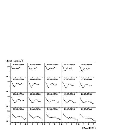
Figure 16: Differential cross sections $\rm d\sigma$/${\rm d}t$ for $\rm\gamma p\rightarrow p\pi^{0}$ . In the range of small values of $|t-t_{\rm{min}}|$ the data were fitted with an exponential function $\rm{e}^{a+b|t-t_{\rm{min}}|}$ distribution.

Fig. 16 shows differential cross sections as functions of the squared four-momentum transfer between the initial photon and the $\pi^{0}$ in the final state. Even though these plots do not provide new information compared to $\rm d\sigma/d\Omega$, they are shown here to emphasize the exponential fall-off of the cross section at low $t$. The differential cross sections are plotted against $|t-t_{\rm min}|$, the difference between the actual momentum transfer and the minimal momentum transfer imposed by kinematics. By definition, the four-momentum transfer is always negative and can range between $t_{\rm min}$ and $t_{\rm max}$, which for $\gamma$p experiments is given by

$$t_{\rm{min/max}} =$$ (18)

$$\left[\frac{m_{\rm{\pi^{0}}}^{2}}{2\sqrt{s}}\right]^{2} -\left[\frac{s-m_{\rm{p}}^{2}}{2\sqrt{s}}\mp\sqrt{\frac{(s+m_{\rm{\pi^{0}}}^{2}-m_{\rm{p}}^{2})^{2}}{4\,s}-m_{\rm{\pi^{0}}}^{2}}\,\,\right]^{2}.$$

Note that $s=m_{\rm p}^{2}+2m_{\rm p}E_{\gamma}$ and that $t_{\rm min}$ corresponds to forward, $t_{\rm{max}}$ to backward production of the $\pi^{0}$.

The squared momentum transfer is related to the emission angle of the pion in the center-of-mass system by

$$t=t_{\rm{min}}- \frac{s-m_{\rm{p}}^{2}}{s}\sqrt{(s-(m_{\pi^{0}}+m_{\rm{p}})^{2})}$$

$$\sqrt{(s-(m_{\pi^{0}}-m_{\rm{p}})^{2})}\sin^{2}\frac{\Theta_{\rm{cms}}}{2}\,.$$ (19)

Differential cross sections d$\sigma$/d$\Omega$ are related to d$\sigma$/d$t$ by

$$\frac{\rm d\sigma}{\rm d\Omega}=\frac{\rm d\sigma}{{\rm d}t}\frac{{\rm d}t}{{\rm d}\Omega}\,.$$ (20)

Using (20), the relation of the two different differential cross sections is given by:

$$\frac{\rm d\sigma}{{\rm d}t}=\frac{4\pi~{}s~{}{\rm d\sigma/d\Omega}}{(s-m_{\rm{p}}^{2})\sqrt{(s-(m_{p}+m_{\rm{\pi^{0}}})^{2})(s-(m_{p}-m_{\rm{\pi^{0}}})^{2})}}.$$ (21)

For small four-momentum transfers, an exponential function is fitted to the distributions shown in Fig. 16. The cross sections fall off according to

$$\frac{{\rm d}\sigma}{{\rm d}t}\propto\exp(a+b\cdot|t-t_{\rm{min}}|),$$ (22)

where the slope parameter $b$ has a negative value.

For large $t$, the cross sections do not exhibit the behavior that would be expected if we had only $t$-channel exchange of mesons. There are structures due to other phenomena, in particular due to formation of $s$-channel resonances. The range, in which the distributions can be fitted by an exponential is not well defined. Nevertheless, we show in Fig. 17 the slope parameter $-b$ of Eq. 22 from the fits as a function of incident photon energy $E_{\gamma}$. With increasing energy, the slope rises to a

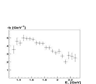
Figure 17: Slope parameter for $\rm\gamma p\rightarrow p\pi^{0}$ from a fit using $\rm{e}^{a+b|t-t_{\rm{min}}|}$ to the differential cross sections $\rm d\sigma$/${\rm d}t$.

maximum value at $E_{\gamma}\sim$1.5–1.6 GeV and then decreases again. At large energies, above 2.2 GeV, the determination of the slope parameter becomes somewhat arbitrary, since the most forward data points at $\cos\Theta_{\rm cm}=0.85$ are missing. For low energies, the slope parameter cannot be determined from the data and can even adopt positive values. Obviously, resonance production is dominant at these energies. The results should hence be interpreted with care. In particular, the turnover at $E_{\gamma}\leq 1.5$ GeV is deduced from very few data points.

7 Summary

We have reported a measurement of unpolarized differential cross sections of the reaction $\rm\gamma p\rightarrow p\pi^{0}$   in the photon energy range from 0.3 GeV to 3.0 GeV, thus completely covering the baryon resonance region. Above 0.8 GeV, the data supersede previous experiments both in solid angle coverage and in statistics. In the mass range above the first resonance region, strong variations of the differential cross sections as functions of photon energy and decay angle in the rest frame of the intermediate state suggest that many partial waves contribute to $\pi^{0}$ photoproduction off protons. This is confirmed by a partial wave analysis which, beyond non-resonant contributions, identifies a series of resonances contributing to the $\rm\gamma p\to p\pi^{0}$ reaction channel. At large photon energies, the angular distributions show a forward rise in $\pi^{0}$ direction signaling dominance of $t$-channel exchange contributions at high energies. The data provide valuable input to coupled-channel isobar-model descriptions of baryons and their excitations. A partial wave analysis reveales a rich spectrum of resonant and non-resonant contributions.

Acknowledgmentss

We thank the technical staff at ELSA and at all the participating institutions for their important contributions to the success of the experiment. We acknowledge financial support from the Deutsche Forschungsgemeinschaft (DFG) within the SFB/TR16. The collaboration with St. Petersburg received funds from DFG and the Russian Foundation for Basic Research. B. Krusche acknowledges support from Schweizerischer Nationalfond.

U. Thoma thanks for an Emmy-Noether grant from the DFG. A. V. Anisovich and A. V. Sarantsev acknowledge support from the Alexander von Humboldt Foundation. This work comprises part of the PhD theses of O. Bartholomy and H. van Pee. Dummy

References

- (1) W. M. Yao et al. [Particle Data Group], J. Phys. G 33 (2006) 1.
-
(2)
S. Capstick and N. Isgur,
Phys. Rev. D 34 (1986) 2809.
S. Capstick and W. Roberts, Prog. Part. Nucl. Phys. 45 (2000) S241. -
(3)
U. Löring, K. Kretzschmar, B. C. Metsch and H. R. Petry,
Eur. Phys. J. A 10 (2001) 309.
U. Löring, B. C. Metsch and H. R. Petry, Eur. Phys. J. A 10 (2001) 395.
U. Löring, B. C. Metsch and H. R. Petry, Eur. Phys. J. A 10 (2001) 447. - (4) D. B. Lichtenberg, Phys. Rev. 178 (1969) 2197.
- (5) E. Klempt, ”Missing resonances”, section 5.3 in Lectures given at 18th Annual Hampton University Graduate Studies (HUGS at JLab 2003), Newport News, Virginia, 2-20 Jun 2003, arXiv:hep-ph/0404270.
- (6) O. Bartholomy et al., Phys. Rev. Lett. 94 (2005) 012003.
- (7) V. Crede et al., Phys. Rev. Lett. 94 (2005) 012004.
- (8) O. Bartholomy et al., ”Photoproduction of mesons off protons”, in preparation.
- (9) A. Anisovich, E. Klempt, A. Sarantsev and U. Thoma, Eur. Phys. J. A 24 (2005) 111.
- (10) A. V. Anisovich et al., Eur. Phys. J. A 25 (2005) 427.
- (11) A. V. Sarantsev et al., Eur. Phys. J. A 25 (2005) 441.
- (12) R. A. Arndt et al., http://gwdac.phys.gwu.edu.
- (13) M. Yoshioka et al., Nucl. Phys. B 168 (1980) 222.
- (14) J. C. Bergstrom, R. Igarashi and J. M. Vogt, Phys. Rev. C 55 (1997) 2016.
- (15) R. Beck et al., Phys. Rev. Lett. 65 (1990) 1841.
- (16) R. Beck et al., Phys. Rev. Lett. 78 (1997) 606.
- (17) M. Fuchs et al., Phys. Lett. B 368 (1996) 20.
- (18) B. Krusche et al., Eur. Phys. J. A 6 (1999) 309.
- (19) A. Schmidt et al., Phys. Rev. Lett. 87 (2001) 232501.
- (20) J. Ahrens et al., Phys. Rev. Lett. 88 (2002) 232002.
-
(21)
S. B. Gerasimov,
Sov. J. Nucl. Phys. 2 (1966) 430
[Yad. Fiz. 2 (1966) 598].
S. D. Drell and A. C. Hearn, Phys. Rev. Lett. 16 (1966) 908. - (22) G. Blanpied et al., Phys. Rev. C 64 (2001) 025203.
- (23) O. Bartalini et al., Eur. Phys. J. A 26 (2005) 399.
- (24) R. A. Arndt et al., Phys. Rev. C 66 (2002) 055213.
- (25) D. Drechsel, O. Hanstein, S. S. Kamalov and L. Tiator, Nucl. Phys. A 645 (1999) 145.
- (26) L. Tiator et al., Eur. Phys. J. A 19, s01 (2004) 55.
- (27) A. Matsuyama, T. Sato and T. S. Lee, “Dynamical coupled-channel model of meson production reactions in the nucleon resonance region,” arXiv:nucl-th/0608051.
- (28) E. Aker et al., Nucl. Instrum. Meth. A 321 (1992) 69.
- (29) G. Suft et al., Nucl. Instrum. Meth. A 538 (2005) 416-424.
- (30) C. Amsler et al., Z. Phys. C 58 (1993) 175.
- (31) B. Krusche et al., Phys. Rev. Lett. 74 (1995) 3736.
-
(32)
A. A. Belyaev et al.,
Nucl. Phys. B 213 (1983) 201.
R. Beck et al., Phys. Rev. Lett. 78 (1997) 606.
D. Rebreyend et al., Nucl. Phys. A 663 (2000) 436. -
(33)
K. H. Althoff et al.,
Z. Phys. C 18 (1983) 199.
E. J. Durwen, BONN-IR-80-7 (1980).
K. Buechler et al., Nucl. Phys. A 570 (1994) 580. - (34) J. Ajaka et al., Phys. Rev. Lett. 81 (1998) 1797.
- (35) K. H. Glander et al., Eur. Phys. J. A 19 (2004) 251.
- (36) R. Lawall et al., Eur. Phys. J. A 24 (2005) 275.
- (37) J. W. C. McNabb et al., Phys. Rev. C 69 (2004) 042201.
- (38) R. G. T. Zegers et al., Phys. Rev. Lett. 91 (2003) 092001.