Financial time-series analysis: A brief overview

1 Introduction

Prices of commodities or assets produce what is called time-series. Different kinds of financial time-series have been recorded and studied for decades. Nowadays, all transactions on a financial market are recorded, leading to a huge amount of data available, either for free in the Internet or commercially. Financial time-series analysis is of great interest to practitioners as well as to theoreticians, for making inferences and predictions. Furthermore, the stochastic uncertainties inherent in financial time-series and the theory needed to deal with them make the subject especially interesting not only to economists, but also to statisticians and physicists tsay . While it would be a formidable task to make an exhaustive review on the topic, with this review we try to give a flavor of some of its aspects.

2 Stochastic methods in time-series analysis

The birth of physics as a science is usually associated with the study of mechanical objects moving with negligible fluctuations, such as the motion of planets. However, this type of systems is not unique, especially at smaller scales where the interaction with the environment and its influence in the form of random fluctuations has to be taken into account. The main theoretical tool to describe the evolution of such systems is the theory of stochastic processes, which can be formulated in various ways: in terms of a Master equation, Fokker-Planck type equation, random walk model, Langevin equation, or through path integrals. Some systems can present unpredictable chaotic behavior due to dynamically generated internal noise. Either truly stochastic or chaotic in nature, noisy processes represent the rule rather than an exception, not only in condensed matter physics but in many fields such as cosmology, geology, meteorology, ecology, genetics, sociology, and economics. In fact the first formulation of the random walk model and a stochastic process was given in the framework of an economic study LB ; Bouchaud2005a . In the following we propose and discuss some questions which we consider as possible land-marks in the field of time series analysis.

2.1 Time-series versus random walk

What if the time-series were similar to a random walk? The answer is: It would not be possible to predict future price movements using the past price movements or trends. Louis Bachelier, who was the first one to investigate this issue in 1900 LB , reached the conclusion that “The mathematical expectation of the speculator is zero” and described this condition as a “fair game.”

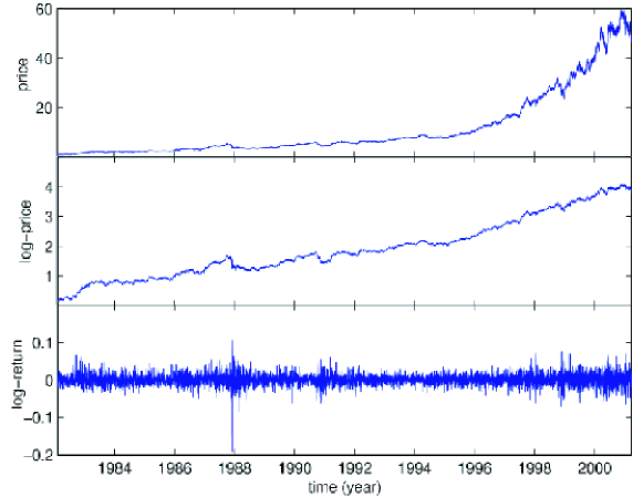
In economics, if $P(t)$ is the price of a stock or commodity at time $t$, then the “log-return” is defined as $r_{\tau}(t)=\ln P(t+\tau)-\ln P(t)$, where $\tau$ is the interval of time. Some statistical features of daily log-return are illustrated in Fig. 1, using the price time-series for the General Electric.

Figure 1: Price in USD (above), log-price (center) and log-return (below) plotted versus time for the General Electric during the period 1982-2000.

The real empirical returns are compared in Fig. 2 with a random time-series we generated using random numbers extracted from a Normal distribution with zero mean and unit standard deviation.

Figure 2: Random time-series, 3000 time steps (above) and Return time-series of the S&P500 stock index, 8938 time steps (below).

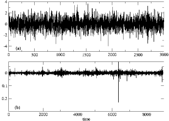
If we divide the time-interval $\tau$ into $N$ sub-intervals (of width $\Delta t$), the total log-return $r_{\tau}(t)$ is by definition the sum of the log-returns in each sub-interval. If the price changes in each sub-interval are independent (Fig. 2 above) and identically distributed with a finite variance, according to the central limit theorem the cumulative distribution function $F(r_{\tau})$ converges to a Gaussian (Normal) distribution for large $\tau$. The Gaussian (Normal) distribution has the following properties: (a) the average and most probable change is zero; (b) the probability of large fluctuations is very low; (c) it is a stable distribution. The distribution of returns was first modeled for “bonds” LB as a Normal distribution,

$$P(r)=\big{[}\sqrt{2\pi}\sigma\big{]}^{-1}\,\exp(-r^{2}/2\sigma^{2})\,,$$

where $\sigma^{2}$ is the variance of the distribution.

In the classical financial theories Normality had always been assumed, until Mandelbrot Man2 and Fama key-250 pointed out that the empirical return distributions are fundamentally different. Namely, they are “fat-tailed” and more peaked compared to the Normal distribution. Based on daily prices in different markets, Mandelbrot and Fama found that $F(r_{\tau})$ was a stable Levy distribution whose tail decays with an exponent $\alpha\simeq 1.7$. This result suggested that short-term price changes were not well-behaved since most statistical properties are not defined when the variance does not exist. Later, using more extensive data, the decay of the distribution was shown to be fast enough to provide finite second moment. With time, several other interesting features of the financial data were unearthed.

The motive of physicists in analyzing financial data has been to find common or universal regularities in the complex time-series (a different approach from those of the economists doing traditional statistical analysis of financial data). The results of their empirical studies on asset price series show that the apparently random variations of asset prices share some statistical properties which are interesting, non-trivial, and common for various assets, markets, and time periods. These are called “stylized empirical facts”.

2.2 “Stylized” facts

Stylized facts are usually formulated using general qualitative properties of asset returns. Hence, distinctive characteristics of the individual assets are not taken into account. Below we consider a few ones from Ref. Cont1 .

1. Fat tails: Large returns asymptotically follow a power law $F(r_{\tau})\sim\left|r\right|^{-\alpha}$, with $\alpha>2$. The values $\alpha=3.01\pm 0.03$ and $\alpha=2.84\pm 0.12$ are found for the positive and negative tail respectively key-43 . An $\alpha>2$ ensures a well-defined second moment and excludes stable laws with infinite variance. There have been various suggestions for the form of the distribution: Student’s-t (Fig. 3), hyperbolic, normal inverse Gaussian, exponentially truncated stable, etc. but there no general consensus has been reached yet

   

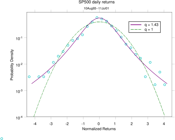
   Figure 3: S&P 500 daily return distribution and normal kernel density estimate. Distributions of log returns normalized by the sample standard deviation rising from the demeaned S & P 500 (circles) and from a Tsallis distribution of index $q=1.43$ (solid line). For comparison, the normal distribution $q=1$ is shown (dashed line). Adapted from Ref. cond-mat/0205078 .

2. Aggregational Normality: As one increases the time scale over which the returns are calculated, their distribution approaches the Normal form. The shape is different at different time scales. The fact that the shape of the distribution changes with $\tau$ makes it clear that the random process underlying prices must have non-trivial temporal structure.

3. Absence of linear auto-correlations: The auto-correlation of log-returns, $\rho(T)\sim\left\langle r_{\tau}(t+T)r_{\tau}(t)\right\rangle$, rapidly decays to zero for $\tau\geq 15$ minutes key-44 , which supports the “efficient market hypothesis” (EMH), discussed in Sec. 2.3. When $\tau$ is increased, weekly and monthly returns exhibit some auto-correlation but the statistical evidence varies from sample to sample.

4. Volatility clustering: Price fluctuations are not identically distributed and the properties of the distribution, such as the absolute return or variance, change with time. This is called time-dependent or “clustered volatility”. The volatility measure of absolute returns shows a positive auto-correlation over a long period of time and decays roughly as a power-law with an exponent between $0.1$ and $0.3$ key-44 ; key-1 ; key-5 . Therefore high volatility events tend to cluster in time, large changes tend to be followed by large changes, and analogously for small changes.

2.3 The Efficient Market Hypothesis (EMH)

A debatable issue in financial econometrics is whether the market is “efficient” or not. The “efficient” asset market is that in which the information contained in past prices is instantly, fully and continually reflected in the asset’s current price. The EMH was proposed by Eugene Fama in his Ph.D. thesis work in the 1960’s, in which he argued that in an active market that consists of intelligent and well-informed investors, securities would be fairly priced and reflect all the information available. Till date there continues to be disagreement on the degree of market efficiency. The three widely accepted forms of the EMH are:

• “Weak” form: all past market prices and data are fully reflected in securities prices and hence technical analysis is of no use.

• “Semistrong” form: all publicly available information is fully reflected in securities prices and hence fundamental analysis is of no use.

• “Strong” form: all information is fully reflected in securities prices and hence even insider information is of no use.

The EMH has provided the basis for much of the financial market research. In the early 1970’s, evidence seemed to be available, supporting the the EMH: the prices followed a random walk and the predictable variations in returns, if any, turned out to be statistically insignificant. While most of the studies in the 1970’s concentrated mainly on predicting prices from past prices, studies in the 1980’s looked at the possibility of forecasting based on variables such as dividend yield, too, see e.g. Ref. FamaFrench . Several later studies also looked at things such as the reaction of the stock market to the announcement of various events such as takeovers, stock splits, etc. In general, results from event studies typically showed that prices seemed to adjust to new information within a day of the announcement of the particular event, an inference that is consistent with the EMH. In the 1990’s, some studies started looking at the deficiencies of asset pricing models. The accumulating evidences suggested that stock prices could be predicted with a fair degree of reliability. To understand whether predictability of returns represented “rational” variations in expected returns or simply arose as “irrational” speculative deviations from theoretical values, further studies have been conducted in the recent years. Researchers have now discovered several stock market “anomalies” that seem to contradict the EMH. Once an anomaly is discovered, in principle, investors attempting to profit by exploiting such an inefficiency should result in the disappearance of the anomaly. In fact, many such anomalies that have been discovered via back-testing, have subsequently disappeared or proved to be impossible to exploit due to high costs of transactions.

We would like to mention the paradoxical nature of efficient markets: if every practitioner truly believed that a market was efficient, then the market would not have been efficient since no one would have then analyzed the behavior of the asset prices. In fact, efficient markets depend on market participants who believe the market is inefficient and trade assets in order to make the most of the market inefficiency.

2.4 Are there any long-time correlations?

Two of the most important and simple models of probability theory and financial econometrics are the random walk and the Martingale theory. They assume that the future price changes only depend on the past price changes. Their main characteristic is that the returns are uncorrelated. But are they truly uncorrelated or are there long-time correlations in the financial time-series? This question has been studied especially since it may lead to deeper insights about the underlying processes that generate the time-series stanley .

Next we discuss two measures to quantify the long-time correlations, and study the strength of trends: the R/S analysis to calculate the Hurst exponent and the detrended fluctuation analysis vandewalle .

Hurst Exponent from R/S Analysis

In order to measure the strength of trends or “persistence” in different processes, the rescaled range (R/S) analysis to calculate the Hurst exponent can be used. One studies the rate of change of the rescaled range with the change of the length of time over which measurements are made. We divide the time-series $\xi_{t}$ of length $T$ into $N$ periods of length $\tau$, such that $N\tau=T$. For each period $i=1,2,...,N$, containing $\tau$ observations, the cumulative deviation is

$$X(\tau)=\sum_{t=(i-1)\tau+1}^{i\tau}\left(\xi_{t}-\left\langle\xi\right\rangle_{\tau}\right),$$ (1)

where $\left\langle\xi\right\rangle_{\tau}$ is the mean within the time-period and is given by

$$\left\langle\xi\right\rangle_{\tau}=\frac{1}{\tau}\sum_{t=(i-1)\tau+1}^{i\tau}\xi_{t}.$$ (2)

The range in the $i$-th time period is given by $R(\tau)=\max X(\tau)-\min X(\tau)$, and the standard deviation is given by

$$S(\tau)=\left[\frac{1}{\tau}\sum_{t=(i-1)\tau+1}^{i\tau}\left(\xi_{t}-\left\langle\xi\right\rangle_{\tau}\right)^{2}\right]^{\frac{1}{2}}.$$ (3)

Then $R(\tau)/S(\tau)$ is asymptotically given by a power-law

$$R(\tau)/S(\tau)=\kappa\tau^{H},$$ (4)

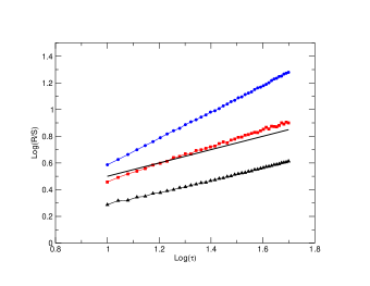
where $\kappa$ is a constant and $H$ the Hurst exponent. In general, “persistent” behavior with fractal properties is characterized by a Hurst exponent $0.5<H\leq 1$, random behavior by $H=0.5$ and “anti-persistent” behavior by $0\leq H<0.5$. Usually Eq. (4) is rewritten in terms of logarithms, $\log(R/S)=H\log(\tau)+\log(\kappa)$, and the Hurst exponent is determined from the slope.

Detrended Fluctuation Analysis (DFA)

In the DFA method the time-series $\xi_{t}$ of length $T$ is first divided into $N$ non-overlapping periods of length $\tau$, such that $N\tau=T$. In each period $i=1,2,...,N$ the time-series is first fitted through a linear function $z_{t}=at+b$, called the local trend. Then it is detrended by subtracting the local trend, in order to compute the fluctuation function,

$$F(\tau)=\left[\frac{1}{\tau}\sum_{t=(i-1)\tau+1}^{i\tau}\left(\xi_{t}-z_{t}\right)^{2}\right]^{\frac{1}{2}}.$$ (5)

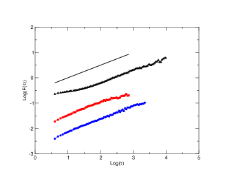
The function $F(\tau)$ is re-computed for different box sizes $\tau$ (different scales) to obtain the relationship between $F(\tau)$ and $\tau$. A power-law relation between $F(\tau)$ and the box size $\tau$, $F(\tau)\sim\tau^{\alpha}$, indicates the presence of scaling. The scaling or “correlation exponent” $\alpha$ quantifies the correlation properties of the signal: if $\alpha=0.5$ the signal is uncorrelated (white noise); if $\alpha>0.5$ the signal is anti-correlated; if $\alpha<0.5$, there are positive correlations in the signal.

Comparison of different time-series

Besides comparing empirical financial time-series with randomly generated time-series, here we make the comparison with multivariate spatiotemporal time-series drawn from coupled map lattices and the multiplicative stochastic process GARCH(1,1) used to model financial time-series.

Multivariate spatiotemporal time-series drawn from coupled map lattices

The concept of coupled map lattices (CML) was introduced as a simple model capable of displaying complex dynamical behavior generic to many spatiotemporal systems kan1 ; kan2 . Coupled map lattices are discrete in time and space, but have a continuous state space. By changing the system parameters, one can tune the dynamics toward the desired spatial correlation properties, many of them already studied and reported kan2 . We consider the class of diffusively coupled map lattices in one-dimension, with sites $i=1,2,\dots,n$, of the form

$$y_{t+1}^{i}=(1-\epsilon)f(y_{t}^{i})+\epsilon[\;f(y_{t}^{i+1})+f(y_{t}^{i-1})\;]/2\,,$$ (6)

where $f(y)=1-ay^{2}$ is the logistic map whose dynamics is controlled by the parameter $a$ and the parameter $\epsilon$ measures the coupling strength between nearest-neighbor sites. We generally choose periodic boundary conditions, $x(n+1)=x(1)$. In the numerical computations reported by Chakraborti and Santhanam chakraborti , a coupled map lattice with $n=500$ was iterated starting from random initial conditions, for $p=5\times 10^{7}$ time steps, after discarding $10^{5}$ transient iterates. As the parameters $a$ and $\epsilon$ are varied, the spatiotemporal map displays various dynamical features like frozen random patterns, pattern selection, space-time intermittency, and spatiotemporal chaos kan2 . In order to study the coupled map lattice dynamics found in the regime of spatiotemporal chaos, where correlations are known to decay rather quickly as a function of the lattice site, the parameters were chosen as $a=1.97$ and $\epsilon=0.4$.

Multiplicative stochastic process GARCH(1,1)

Considerable interest has been in the application of ARCH/GARCH models to financial time-series, which exhibit periods of unusually large volatility followed by periods of relative tranquility. The assumption of constant variance or “homoskedasticity” is inappropriate in such circumstances. A stochastic process with auto-regressional conditional “heteroskedasticity” (ARCH) is actually a stochastic process with “non-constant variances conditional on the past but constant unconditional variances” engle . The ARCH($p$) process is defined by the equation

$$\sigma_{t}^{2}=\alpha_{0}+\alpha_{1}x_{t-1}^{2}+...+\alpha_{p}x_{t-p}^{2}\,,$$ (7)

where the $\{\alpha_{0},\alpha_{1},...\alpha_{p}\}$ are positive parameters and $x_{t}$ is a random variable with zero mean and variance $\sigma_{t}^{2}$, characterized by a conditional probability distribution function $f_{t}(x)$, which may be chosen as Gaussian. The nature of the memory of the variance $\sigma_{t}^{2}$ is determined by the parameter $p$.

The generalized ARCH process GARCH($p,q$) was introduced by Bollerslev bollerslev and is defined by the equation

$$\sigma_{t}^{2}=\alpha_{0}+\alpha_{1}x_{t-1}^{2}+...+\alpha_{q}x_{t-q}^{2}+\beta_{1}\sigma_{t-1}^{2}+...+\beta_{p}\sigma_{t-p}^{2}\,,$$ (8)

where $\{\beta_{1},...,\beta_{p}\}$ are additional control parameters.

The simplest GARCH process is the GARCH(1,1) process, with Gaussian conditional probability distribution function ,

$$\sigma_{t}^{2}=\alpha_{0}+\alpha_{1}x_{t-1}^{2}+\beta_{1}\sigma_{t-1}^{2}\,.$$ (9)

The random variable $x_{t}$ can be written in term of $\sigma_{t}$ defining $x_{t}\equiv\eta_{t}\sigma_{t}$, where $\eta_{t}$ is a random Gaussian process with zero mean and unit variance. One can rewrite Eq. 9 as a random multiplicative process

$$\sigma_{t}^{2}=\alpha_{0}+(\alpha_{1}\eta_{t-1}^{2}+\beta_{1})\sigma_{t-1}^{2}\,.$$ (10)

DFA analysis of auto-correlation function of absolute returns

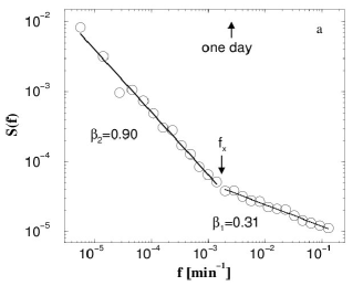
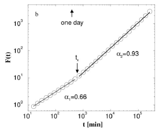
The analysis of financial correlations was done in 1997 by the group of H.E. Stanley key-1 . The correlation function of the financial indices of the New York stock exchange and the S&P 500 between January, 1984 and December, 1996 were analyzed at one minute intervals. The study confirmed that the auto-correlation function of the returns fell off exponentially but the absolute value of the returns did not. Correlations of the absolute values of the index returns could be described through two different power laws, with crossover time $t_{\times}\approx 600$ minutes, corresponding to $1.5$ trading days. Results from power spectrum analysis and DFA analysis were found to be consistent. The power spectrum analysis of Fig. 4 yielded exponents $\beta_{1}=0.31$ and $\beta_{2}=0.90$ for $f>f_{\times}$ and $f<f_{\times}$, respectively. This is consistent with the result that $\alpha=(1+\beta)/2$ and $t_{\times}\approx 1/f_{\times}$, as obtained from detrended fluctuation analysis with exponents $\alpha_{1}=0.66$ and $\alpha_{2}=0.93$ for $t<t_{\times}$ and $t>t_{\times}$, respectively.

Figure 4: Power spectrum analysis (left) and detrended fluctuation analysis (right) of auto-correlation function of absolute returns, from Ref. key-1 .

Numerical Comparison

In order to provide an illustrative example, in Fig. 5 a comparison among various analysis techniques and process is presented, while the values of the exponents of the Hurst and DFA analyzes are listed in Table 1. For the numerical computations reported by Chakraborti and Santhanam chakraborti , the parameter values chosen were $\alpha_{0}=0.00023$, $\alpha_{1}=0.09$ and $\beta_{0}=0.01$.

Figure 5: R/S (left) and DFA (right) analyses: Random time-series, 3000 time steps (black solid line); multivariate spatiotemporal time-series drawn from coupled map lattices with parameters $a=1.97$ and $\epsilon=0.4$, 3000 time steps (black filled up-triangles); multiplicative stochastic process GARCH(1,1) with parameters $\alpha_{0}=0.00023$, $\alpha_{1}=0.09$ and $\beta_{0}=0.01$, 3000 time steps (red filled squares); Return time-series of the S&P500 stock index, 8938 time steps (blue filled circles).

Table 1: Hurst and DFA exponents.

Process	Hurst exponent	DFA exponent
Random	0.50	0.50
Chaotic (CML)	0.46	0.48
GARCH(1,1)	0.63	0.51
Financial Returns	0.99	0.51

3 Random Matrix methods in time-series analysis

The R/S and the detrended fluctuation analysis considered in the previous section are suitable for analyzing univariate data. Since the stock-market data are essentially multivariate time-series data, it is worth constructing a correlation matrix to study its spectra and contrasting it with random multivariate data from coupled map lattice. Empirical spectra of correlation matrices, drawn from time-series data, are known to follow mostly random matrix theory (RMT) gopi .

3.1 Correlation matrix and Eigenvalue density

Correlation matrix

Financial Correlation matrix

If there are $N$ assets with a price $P_{i}(t)$ for asset $i$ at time $t$, the logarithmic return of stock $i$ is $r_{i}(t)=\ln P_{i}(t)-\ln P_{i}(t-1)$. A sequence of such values for a give period of time forms the return vector $\boldsymbol{r}_{i}$. In order to characterize the synchronous time evolution of stocks, one defines the equal time correlation coefficients between stocks $i$ and $j$,

$$\rho_{ij}=\Big{[}\langle\boldsymbol{r}_{i}\boldsymbol{r}_{j}\rangle-\langle\boldsymbol{r}_{i}\rangle\langle\boldsymbol{r}_{j}\rangle\Big{]}\Big{/}\sqrt{[\langle\boldsymbol{r}_{i}^{2}\rangle-\langle\boldsymbol{r}_{i}\rangle^{2}][\langle\boldsymbol{r}_{j}^{2}\rangle-\langle\boldsymbol{r}_{j}\rangle^{2}]}\,,$$ (11)

where $\left\langle...\right\rangle$ indicates a time average over the trading days included in the return vectors. The correlation coefficients $\rho_{ij}$ form an $N\times N$ matrix, with $-1\leq\rho_{ij}\leq 1$. If $\rho_{ij}=1$, the stock price changes are completely correlated; if $\rho_{ij}=0$, the stock price changes are uncorrelated and if $\rho_{ij}=-1$, then the stock price changes are completely anti-correlated.

Correlation matrix from spatiotemporal series from coupled map lattices

Consider a time-series of the form $z^{\prime}(x,t)$, where $x\!=\!1,2,\dots,n$ and $t\!=\!1,2,\dots,p$ denote the discretized space and time. In this way, the time-series at every spatial point is treated as a different variable. We define

$$z(x,t)=\big{[}z^{\prime}(x,t)-\langle z^{\prime}(x)\rangle\big{]}\big{/}{\sigma(x)}\,,$$ (12)

as the normalized variable, with the brackets $\langle.\rangle$ representing a temporal average and $\sigma(x)$ the standard deviation of $z^{\prime}$ at position $x$. Then, the equal-time cross-correlation matrix can be written as

$$S_{x,x^{\prime}}=\langle z(x,t)\,z(x^{\prime},t)\rangle\,,~{}~{}~{}~{}~{}~{}x,x^{\prime}=1,2,\dots,n\,.$$ (13)

This correlation matrix is symmetric by construction. In addition, a large class of processes is translationally invariant and the correlation matrix will possess the corresponding symmetry. We use this property for our correlation models in the context of coupled map lattices. In time-series analysis, the averages $\langle.\rangle$ have to be replaced by estimates obtained from finite samples. We use the maximum likelihood estimates, i.e., $\langle a(t)\rangle\approx\frac{1}{p}\sum_{t=1}^{p}a(t)$. These estimates contain statistical uncertainties which disappear for $p\to\infty$. Ideally we require $p\gg n$ to have reasonably correct correlation estimates.

Eigenvalue Density

The interpretation of the spectra of empirical correlation matrices should be done carefully in order to distinguish between system specific signatures and universal features. The former ones express themselves in a smoothed level density, whereas the latter ones are usually represented by the fluctuations on top of such a smooth curve. In time-series analysis, matrix elements are not only prone to uncertainties such as measurement noise on the time-series data, but also to the statistical fluctuations due to finite sample effects. When characterizing time series data in terms of RMT, we are not interested in these sources of fluctuations, which are present on every data set, but we want to identify the significant features which would be shared, in principle, by an “infinite” amount of data without measurement noise. The eigenfunctions of the correlation matrices constructed from such empirical time-series carry the information contained in the original time-series data in a “graded” manner and provide a compact representation for it. Thus, by applying an approach based on RMT, we try to identify non-random components of the correlation matrix spectra as deviations from RMT predictions gopi .

We now consider the eigenvalue density, studied in applications of RMT methods to time-series correlations. Let ${\mathcal{N}}(\lambda)$ be the integrated eigenvalue density, giving the number of eigenvalues smaller than a given $\lambda$. The eigenvalue or level density, $\rho(\lambda)=d\mathcal{N}(\lambda)/d\lambda$, can be obtained assuming a random correlation matrix mitra . Results are found to be in good agreement with the empirical time-series data from stock market fluctuations plerou . From RMT considerations, the eigenvalue density for random correlations is given by

$$\rho_{rmt}(\lambda)=[Q/(2\pi\lambda)]\sqrt{{(\lambda_{max}-\lambda})({\lambda-\lambda_{min}})}\,.$$ (14)

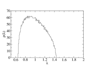
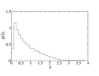
Here $Q\!=\!N/T$ is the ratio of the number of variables to the length of each time-series, while $\lambda_{min}=1+1/Q-2\sqrt{1/Q}$ and $\lambda_{max}=1+1/Q+2\sqrt{1/Q}$ represent the minimum and maximum eigenvalues of the random correlation matrix. The presence of correlations in the empirical correlation matrix produces a violation of this form of eigenvalue density, for a certain number of dominant eigenvalues, often corresponding to system specific information in the data. As examples, Fig. 6 shows the eigenvalue densities for S&P500 data and for the chaotic data from coupled map lattice are shown: the curves are qualitatively different from the form of Eq. (14).

Figure 6: Spectral density for multivariate spatiotemporal time-series drawn from coupled map lattices (left) and eigenvalue density for the return time-series of the S&P500 stock market data, 8938 time steps (right).

3.2 Earlier estimates and studies using Random Matrix Theory (RMT)

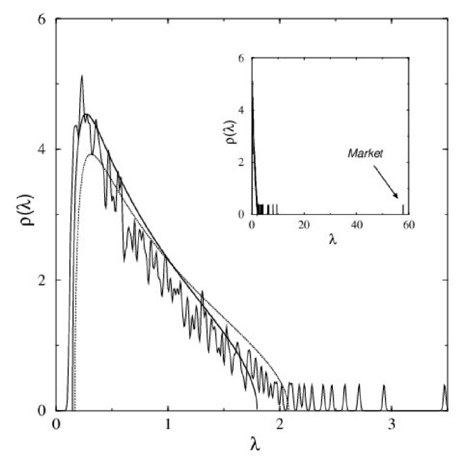
Laloux et al. key-4 showed that results from RMT were useful to understand the statistical structure of the empirical correlation matrices appearing in the study of price fluctuations. The empirical determination of a correlation matrix is a difficult task. If one considers $N$ assets, the correlation matrix contains $N(N-1)/2$ mathematically independent elements, which must be determined from $N$ time-series of length $T$. If $T$ is not very large compared to $N$, then generally the determination of the covariances is noisy, and therefore the empirical correlation matrix is to a large extent random. The smallest eigenvalues of the matrix are the most sensitive to this “noise”. But the eigenvectors corresponding to these smallest eigenvalues determine the minimum risk portfolios in Markowitz’s theory. It is thus important to distinguish “signal” from “noise” or, in other words, to extract the eigenvectors and eigenvalues of the correlation matrix, containing real information (which is important for risk control), from those which do not contain any useful information and are unstable in time. It is useful to compare the properties of an empirical correlation matrix to a “null hypothesis” — a random matrix which arises for example from a finite time-series of strictly uncorrelated assets. Deviations from the random matrix case might then suggest the presence of true information. The main result of the study was a remarkable agreement between theoretical predictions, based on the assumption that the correlation matrix is random, and empirical data concerning the density of eigenvalues. This is shown in Fig. 7 for the time-series of the different stocks of the S&P 500 (or other stock markets).

Figure 7: Eigenvalue spectrum of the correlation matrices, adapted from Ref. key-4 .

Cross-correlations in financial data were also studied by Plerou et al. key-2 , who analyzed price fluctuations of different stocks through RMT. Using two large databases, they calculated cross-correlation matrices of returns constructed from: (i) 30-min returns of 1000 US stocks for the period 1994–95; (ii) 30-min returns of 881 US stocks for the period 1996–97; (iii) 1-day returns of 422 US stocks for the period 1962–96. They tested the statistics of the eigenvalues $\lambda_{i}$ of cross-correlation matrices against a “null hypothesis” and found that a majority of the eigenvalues of the cross-correlation matrices were within the RMT bounds $(\lambda_{min},\lambda_{max})$ defined above for random correlation matrices. Furthermore, they analyzed the eigenvalues of the cross-correlation matrices within the RMT bound for universal properties of random matrices and found good agreement with the results for the Gaussian orthogonal ensemble (GOE) of random matrices, implying a large degree of randomness in the measured cross-correlation coefficients. It was found that: (i) the distribution of eigenvector components, for the eigenvectors corresponding to the eigenvalues outside the RMT bound, displayed systematic deviations from the RMT prediction; (ii) such “deviating eigenvectors” were stable in time; (iii) the largest eigenvalue corresponded to an influence common to all stocks; (iv) the remaining deviating eigenvectors showed distinct groups, whose identities corresponded to conventionally-identified business sectors.

4 Approximate Entropy method in time-series analysis

The Approximate Entropy (ApEn) method is an information theory-based estimate of the complexity of a time series introduced by S. Pincus Pincus1991a , formally based on the evaluation of joint probabilities, in a way similar to the entropy of Eckmann and Ruelle. The original motivation and main feature, however, was not to characterize an underlying chaotic dynamics, rather to provide a robust model-independent measure of the randomness of a time series of real data, possibly — as it is usually in practical cases — from a limited data set affected by a superimposed noise. ApEn has been used by now to analyze data obtained from very different sources, such as digits of irrational and transcendental numbers, hormone levels, clinical cardiovascular time-series, anesthesia depth, EEG time-series, and respiration in various conditions.

Given a sequence of $N$ numbers $\{u(j)\}=\{u(1),u(2),\dots,u(N)\}$, with equally spaced times $t_{j+1}-t_{j}\equiv\Delta t=\mathrm{const}$, one first extracts the sequences with embedding dimension $m$, i.e., $x(i)=\{u(i),u(i+1),\dots,u(i+m-1)\}$, with $1\leq i\leq N-m+1$. The ApEn is then computed as

$$\mathrm{ApEn}=\Phi^{m}(r)-\Phi^{m+1}(r)\,,$$ (15)

where $r$ is a real number representing a threshold distance between series, and the quantity $\Phi^{m}(r)$ is defined as

$$\Phi^{m}(r)=\langle\ln[C_{i}^{m}(r)]\rangle=\sum_{i=1}^{N-m+1}\ln[C_{i}^{m}(r)]/(N-m+1)\,.$$ (16)

Here $C_{i}^{m}(r)$ is the probability that the series $x(i)$ is closer to a generic series $x(j)$ ($j\leq N-m+1$) than the threshold $r$,

$$C_{i}^{m}(r)=\mathcal{N}[d(i,j)\leq r]/(N-m+1)\,,$$ (17)

with $\mathcal{N}[d(i,j)\leq r]$ the number of sequences $x(j)$ close to $x(i)$ less than $r$. As definition of distance between two sequences, the maximum difference (in modulus) between the respective elements is used,

$$d(i,j)=\max_{k=1,2,\dots,m}(|u(j+k-1)-u(i+k-1)|)\,.$$ (18)

Quoting Pincus and Kalman Pincus2004a , “…ApEn measures the logarithmic frequency that runs of patterns that are close (within $r$) for $m$ contiguous observations remain close (within the same tolerance width $r$) on the next incremental comparison”. Comparisons are intended to be done at fixed $m$ and $r$, the general ApEn($m$,$r$) being in fact a family of parameters.

In economics, the ApEn method has been shown to be a reliable estimate of the efficiency of market Pincus1991a ; Pincus2004a ; Pincus1996a and has been applied to various economically relevant events. For instance, the ApEn computed for the S&P 500 index has shown a drastic increase in the two-week period preceding the stock market crash of 1987. Just before the Asian crisis of November 1997, the ApEn computed for the Hong Kong’s Hang Seng index, from 1992 to 1998, assumes its highest values. More recently, a broader investigation carried out for various countries through the ApEn by Oh, Kim, and Eom, revealed a systematic difference between the efficiencies of the markets between the period before and after the the Asian crisis Oh2006a .

References

- (1) R.S. Tsay, Analysis of Financial Time Series, John Wiley, New York (2002).
- (2) L. Bachelier, Theorie de la speculation. Annales Scientifiques de l’Ecole Normale Superieure, Suppl. 3, No. 1017, 21-86 (1900). English translation by A. J. Boness in: P. Cootner (Ed.), The Random Character of Stock Market Prices, Page 17, MIT, Cambridge, MA, (1967).
- (3) J.-P. Bouchaud, CHAOS 15, 026104 (2005).
- (4) B.B. Mandelbrot, J. Business 36, 394 (1963).
- (5) E. Fama, J. Business 38, 34 (1965).
- (6) R. Cont, Quant. Fin. 1, 223 (2001).
- (7) L. Borland, arxiv:cond-mat/0205078.
- (8) P. Gopikrishnan, M. Meyer, L.A.N. Amaral, H.E. Stanley, Eur. Phys. J. B 3, 139 (1998).
- (9) R. Cont, M. Potters, J.-P. Bouchaud, in: B. Dubrulle, F. Graner and D. Sornette (Eds.), Scale Invariance and Beyond (Proc. CNRS Workshop on Scale Invariance, Les Houches, 1997), Springer, Berlin (1997).
- (10) Y. Liu, P. Cizeau, M. Meyer, C.-K. Peng, H.E. Stanley, Physica A 245, 437 (1997); arxiv:cond-mat/9706021.
- (11) P. Cizeau, Y. Liu, M. Meyer, C.-K. Peng, H.E. Stanley, Physica A 245, 441 (1997).
- (12) E.F. Fama, K.R. French, J. Fin. Economics 22, 3 (1988).
- (13) R.N. Mantegna, H.E. Stanley, An Introduction to Econophysics, Cambridge University Press, New York (2000).
- (14) N. Vandewalle, M. Ausloos, Physica A 246, 454 (1997). C.-K. Peng, S.V. Buldyrev, S. Havlin, M. Simons, H.E. Stanley, A.L. Goldberger, Phys. Rev. E 49, 1685 (1994). Y. Liu, P. Gopikrishnan, P. Cizeau, M. Meyer, C.-K.. Peng, H.E. Stanley, Phys. Rev. E 60, 1390 (1999). M. Beben, A. Orlowski, Eur. Phys. J. B 20, 527 (2001). A. Sarkar, P. Barat, Physica A 364, 362 (2006); arxiv:physics/0504038. P. Norouzzadeh, B. Rahmani, Physica A 367, 328 (2006); D. Wilcox, T. Gebbie, arxiv:cond-mat/0404416.
- (15) See K. Kaneko (Ed.), Theory and Applications of Coupled Map Lattices, Wiley, New York (1993), and in particular the contribution of R. Kapral.
- (16) K. Kaneko, Physica D 34, 1 (1989).
- (17) A. Chakraborti, M.S. Santhanam, Int. J. Mod. Phys. C 16, 1733 (2005).
- (18) R.F. Engle, Econometrica 50, 987 (1982).
- (19) T. Bollerslev, J. Econometrics 31, 307 (1986).
- (20) P. Gopikrishnan, B. Rosenow, V. Plerou, H.E. Stanley, Phys. Rev. E 64, 035106 (2001).
- (21) A.M. Sengupta, P.P. Mitra, Phys. Rev. E 60, 3389 (1999).
- (22) V. Plerou, P. Gopikrishnan, B. Rosenow, L.A.N. Amaral, T. Guhr, H.E. Stanley, Phys. Rev. E 65, 066126 (2002).
- (23) L. Laloux, P. Cizeau, J.-P. Bouchaud, M. Potters, Phys. Rev. Lett. 83, 1467 (1999); arxiv:cond-mat/9810255.
- (24) V. Plerou, P. Gopikrishnan, B. Rosenow, L.A.N. Amaral, H.E. Stanley, Phys. Rev. Lett. 83, 1471 (1999); arxiv:cond-mat/9902283. V. Plerou, P. Gopikrishnan, B. Rosenow, L.A.N. Amaral, T. Guhr, H.E. Stanley, Phys. Rev. E 65, 066126 (2002); arxiv:cond-mat/0108023.
- (25) S. M. Pincus, Proc. Nati. Acad. Sci. USA 88, 2297 (1991).
- (26) S. Pincus, R.E. Kalman, Proc. Nati. Acad. Sci. USA 101, 13709 (2004).
- (27) S. Pincus, B.H. Singer, Proc. Nati. Acad. Sci. USA 93, 2083 (1996).
- (28) G. Oh, S. Kim, C. Eom, Market efficiency in foreign exchange markets, Physica A, in press.