Magneto-oscillations due to electron-electron interactions in the ac conductivity of a 2D electron gas

Abstract

Electron-electron interactions give rise to the correction, $\delta\sigma^{int}(\omega),$ to the ac magnetoconductivity, $\sigma(\omega)$, of a clean 2D electron gas that is periodic in $\omega_{c}^{-1}$, where $\omega_{c}$ is the cyclotron frequency. Unlike conventional harmonics of the cyclotron resonance, which are periodic with $\omega$, this correction is periodic with $\omega^{3/2}$. Oscillations in $\delta\sigma^{int}(\omega)$ develop at low magnetic fields, $\omega_{c}\ll\omega$, when the conventional harmonics are suppressed by the disorder. Their origin is a double backscattering of an electron from the impurity-induced Friedel oscillations. During the time $\sim\omega^{-1}$ between the two backscattering events the electron travels only a small portion of the Larmour circle.

Introduction. Originally, the cyclotron resonance (and its harmonics) in the ac conductivity, $\sigma(\omega)$, of the 2D electron gas had been detected by measuring the transmission of the microwave radiation koch74 . In the recent experiment on high-mobility samples zudov01 , it was demonstrated that this resonance, together with harmonics, also manifests itself in the dc magnetoresistance under microwave illumination, i.e., in the photoconductivity. A spectacular strength of this effect, and, in particular, observation of the zero-resistance state, above a certain intensity of illumination zudov03 ; mani02 ; dorozhkin03 , had attracted a steady interest of the researchers to the ac-response of a high-mobility electron gas in a weak magnetic field, $B$. Unlike the conventional Shubnikov-de Haas oscillations of the dc magnetoresistance, which vanish with temperature as $\exp(-2\pi^{2}T/\omega_{c})$, where $\omega_{c}$ is the cyclotron quantum, the magneto-oscillations of $\sigma(\omega)$ survive at high temperature mirlin03 ; mirlin04 . The shape of these oscillations is given by mirlin03 ; mirlin04

$$\frac{\delta\sigma_{\pm}(\omega)}{\sigma_{\pm}(\omega)}=2\cos\Biggl{(}\frac{2\pi\omega}{\omega_{c}}\Biggr{)}\exp\left(-\frac{2\pi}{\omega_{c}\tau}\right),$$ (1)

where $\tau$ is the scattering time, and $\sigma_{\pm}(\omega)$ is related to the dc conductivity $\sigma_{0}$ as $\sigma_{\pm}(\omega)={\sigma_{0}}/{\left[2+2(\omega\pm\omega_{c})^{2}\tau^{2}\right]}$. Classically, the meaning of the damping factor $\delta^{2}=\exp\bigl{(}-2\pi/\omega_{c}\tau\bigr{)}<1$ is the probability for an electron to execute the entire Larmour circle, $2\pi R_{\mbox{\tiny L}}$, without being scattered. Oscillations Eq. (1) is a single-electron effect. In converting of these oscillations into the oscillating dc photoconductivity mirlin04 ; vavilov04 ; mirlin05 ; long , the electron-electron interactions enter as a source of relaxation of the oscillatory part of the distribution function.

In the present paper we demonstrate that interactions by themselves give rise to the oscillatory contribution, $\delta\sigma^{int}(\omega)$, to the linear ac conductivity, $\sigma(\omega)$, at frequencies much higher than in Eq. (1). To contrast this contribution to Eq. (1), we present $\delta\sigma^{int}(\omega)$ in the form

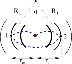
Figure 1: Illustration of the $B$-dependent contribution, $\delta\Theta_{\mbox{\tiny B}}(r)$, to the phase of the polarization operator; $R_{\mbox{\tiny L}}[\theta-2\sin(\theta/2)]$ is the elongation of the semiclassical trajectory due to the field-induced curving. The origin of oscillating magnetoconductivity is the scattering from the Friedel oscillations (arcs of decreasing thickness), at points 1 and 2, located symmetrically with respect to the impurity shown with a big dot.

$$\!\frac{\delta\sigma^{int}(\omega)}{\sigma(\omega)}\propto\cos\Biggl{(}\!\!\!\! C \!\!\!\!{}_{\omega}\frac{\omega}{\omega_{c}}-\frac{\pi}{4}\Biggr{)}\exp\left[-\frac{3C_{\omega}}{\omega_{c}}\left(\frac{1}{\tau}+2\pi T\right)\right],$$

where

$$C_{\omega}=\left[\frac{32\omega}{27E_{\mbox{\tiny F}}}\right]^{1/2},$$ (3)

and $E_{\mbox{\tiny F}}$ is the Fermi energy. Since $C_{\omega}$ is small, the correction Eq. (Magneto-oscillations due to electron-electron interactions in the ac conductivity of a 2D electron gas) develops oscillations at much smaller magnetic fields $\omega_{c}\sim C_{\omega}\omega\ll\omega$ than Eq. (1). At such fields, the damping factor in Eq. (1) is $\sim\exp\left(-2\pi/C_{\omega}\right)$, i.e., the conventional oscillations are completely washed out.

Qualitative picture. The origin of the oscillations Eq. (Magneto-oscillations due to electron-electron interactions in the ac conductivity of a 2D electron gas) lies in a peculiar modification by the interactions of the impurity scattering in a weak magnetic field. Conventionally, Dolgopolov ; Narozhny ; gornyi04 this modification amounts to the additional scattering rudin from the Friedel oscillations of the electron density, created by the impurity. Such a modification does not lead to the anomalous sensitivity to low $B$. However, as we demonstrate below, this sensitivity emerges in the second order in the electron-electron interaction strength. The corresponding second-order processes are illustrated in Figs. 1 and 2. They are: (i). Photoexcited electron emits a virtual pair, which is subsequently annihilated. Impurity scatters not the original electron, but rather the impurity scattering occurs between the states, constituting the pair, prior to annihilation. Diagram $b$ in Fig. 2 describes this process. (ii) Electron is not scattered directly by the impurity, but rather experiences a double backscattering from the impurity-induced Friedel oscillations, as illustrated in Fig. 1, and also by the diagram $a$ in Fig. 2.

Figure 2: Diagrams contributing to the second-order interaction correction to the ac magnetoconductivity. Dashed lines denote the impurity scattering. Dots in the vertices combine two types of the interaction matrix elements, as shown in the left inset. Diagrams b and e describe the impurity scattering of the secondary electron (hole); other diagrams describe double scattering of photoexcited electron (hole) by the Friedel oscillation. Right inset: diagram (a) for purely disorder-induced part of the self-energy, $\Sigma_{n}$, is plotted together with representative diagrams (b) and (c) for the interaction-induced self-energy, $\delta\Sigma_{n}^{int}$. Only diagrams (c), describing two electron-electron scattering processes, contribute to the interaction-induced magneto-oscillations.

We demonstrate that the corrections to the conductivity from both these processes oscillate with magnetic field according to Eq. (Magneto-oscillations due to electron-electron interactions in the ac conductivity of a 2D electron gas). The oscillations reflect the fact that, for both processes, the dominant contribution to the double backscattering cross-section comes from two “distinguished” points that are located symmetrically with respect to the impurity at certain well-defined distance, $r_{\omega}\sim C_{\omega}R_{\mbox{\tiny L}}$, see Fig. 1. Then the argument of the cosine in Eq. (Magneto-oscillations due to electron-electron interactions in the ac conductivity of a 2D electron gas) can be interpreted as a product $\omega t_{\omega}$, where $t_{\omega}=r_{\omega}/v_{\mbox{\tiny F}}$ is the time, during which the electron with Fermi velocity, $v_{\mbox{\tiny F}}$, travels the distance $r_{\omega}$.

Derivation. Although the interaction-induced oscillations come from small distances, $r_{\omega}\ll R_{\mbox{\tiny L}}$, we nevertheless will evaluate $\sigma(\omega)$ in the Landau gauge to demonstrate how both oscillations Eq. (1) and Eq. (Magneto-oscillations due to electron-electron interactions in the ac conductivity of a 2D electron gas) emerge from the same calculation. Within the self-consistent Born approximation, averaging in the general expression for the diagonal conductivity

$$\sigma(\omega)=\frac{-e^{2}}{4\pi^{3}\Omega}\int\limits_{-\infty}^{\infty}\!\!\frac{d\epsilon}{\omega}\left(f_{\epsilon}-f_{\epsilon+\omega}\right)\text{Tr}{\overline{{\hat{v}_{x}}\text{Im}{\hat{G}}_{\epsilon+\omega}{\hat{v}_{x}}\text{Im}{\hat{G}}_{\epsilon}}}$$ (4)

is decoupled into two averaged Green functions

$$G_{\epsilon}=\sum_{n}G_{n}(\epsilon)=\sum_{n}\frac{1}{\epsilon-\epsilon_{n}-\Sigma_{n}(\epsilon)},$$ (5)

where $\epsilon_{n}=(n+\frac{1}{2})\hbar\omega_{c}$ are the Landau levels, and $\Sigma_{n}(\epsilon)$ is the self-energy. In Eq. (4), the bar denotes the disorder averaging, $\Omega$ is the normalization area, and $f_{\epsilon}$ is the Fermi distribution. Upon decoupling, Eq. (4) takes a familiar form

$$\sigma_{\pm}(\omega)=\frac{e^{2}v_{\mbox{\tiny F}}^{2}\omega_{c}\nu_{0}}{8\pi}\int\!\frac{d\epsilon}{\omega}\Bigl{(}f_{\epsilon}-f_{\epsilon+\omega}\Bigr{)}$$

$$\times\sum_{n}\text{Im}G_{n\pm 1}(\epsilon+\omega)\;\text{Im}G_{n}(\epsilon),\qquad\qquad\qquad$$ (6)

where $\nu_{0}$ is the 2D density of states. For high Landau levels, $\left(E_{\mbox{\tiny F}}/\hbar\omega_{c}\right)\gg 1$, in the first approximation in $\delta<1$, the self-energy can be replaced by its zero-field value, $i/2\tau$. Then Eq. (Magneto-oscillations due to electron-electron interactions in the ac conductivity of a 2D electron gas) readily reproduces the Drude conductivity. In order to capture the oscillatory ac magnetoconductivity, in the next approximation, one should take into account the “quantum” correction, $\delta\Sigma_{n}^{Q}(\epsilon)\propto\delta\exp\left(-2\pi i\epsilon/\omega_{c}\right)$, to the self-energy due to the discreteness of the Landau levels, as well as the interaction correction, $\delta\Sigma_{n}^{int}(\epsilon)$. Since both corrections are smaller than $1/\tau$, they cause a small correction to the Green functions Eq. (5) of the form

$$\delta G_{n}(\epsilon)=\frac{\delta\Sigma_{n}^{Q}(\epsilon)+\delta\Sigma_{n}^{int}}{\left(\epsilon-\epsilon_{n}-\frac{i}{2\tau}\right)^{2}}.$$ (7)

The first and the second terms in Eq. (7) give rise to the oscillations Eq. (1) and Eq. (Magneto-oscillations due to electron-electron interactions in the ac conductivity of a 2D electron gas), respectively. However, to reproduce these oscillations the “quantum” and the interaction corrections should be handled differently. To reproduce Eq. (1), upon substituting Eq. (7) into Eq. (Magneto-oscillations due to electron-electron interactions in the ac conductivity of a 2D electron gas), one should keep the product, $\delta\Sigma_{n+1}^{Q}(\epsilon+\omega)\bigl{[}\delta\Sigma_{n}^{Q}(\epsilon)\bigr{]}^{\ast}$. It contains the oscillating term $\propto\exp\left(-2\pi i\omega/\omega_{c}\right)$, which does not depend neither on $n$ nor on $\epsilon$. For this reason, the resulting oscillations of magnetoconductivity are $T$-independent. By contrast, to capture the interaction-induced oscillations, it is sufficient to keep $\delta\Sigma_{n}^{int}$ only in one of the Green functions in Eq. (Magneto-oscillations due to electron-electron interactions in the ac conductivity of a 2D electron gas), and its $n$-dependence is crucial. We will perform further calculation for $\delta\Sigma_{n}^{int}(\epsilon)$ given by the first diagram of type $c$ in Fig. 2 (inset). This is because the diagrams of type $b$ do not cause magneto-oscillations, while the contributions of other diagrams of type $c$ are comparable to that of the first one, and will be addressed later.

The first diagram of type $c$ can be presented as

$$\delta\Sigma_{n}^{int}(\epsilon)=\sum_{m}\frac{|R_{nm}|^{2}}{\epsilon-\epsilon_{m}+\frac{i}{2\tau}},$$ (8)

so that the $n$-dependence is encoded in the “matrix elements”, $R_{nm}$. Substituting Eq. (8) into Eq. (7), and then Eq. (7) into Eq. (Magneto-oscillations due to electron-electron interactions in the ac conductivity of a 2D electron gas) yields

$$\delta \!\!\!\!\!\!\sigma^{int}(\omega)\propto\int\frac{d\epsilon}{\omega}\bigl{(}f_{\epsilon}-f_{\epsilon+\omega}\bigr{)}\times\!\!\!\!$$

Im $$\!\!\sum_{n,m}\frac{|R_{nm}|^{2}}{\left(\epsilon-\epsilon_{n}+\frac{i}{2\tau}\right)^{2}\left(\epsilon+\omega-\epsilon_{n\pm 1}-\frac{i}{2\tau}\right)\left(\epsilon-\epsilon_{m}+\frac{i}{2\tau}\right)}.$$

As a next step, we express the matrix element, $R_{nm}$, as an integral in the coordinate space, following Fig. 2c, $R_{nm}\propto\int d{\bf r}\psi_{n}^{\ast}({\bf r})\psi_{m}({\bf r})\Pi_{0}({\bf r},0)$, where $\Pi_{0}({\bf r},0)$ is the static polarization operator between the point ${\bf r}=0$, where the impurity is located, and the point ${\bf r}$, where the backscattering takes place. Our prime observation is that with such $R_{nm}$ the relevant term in Eq. (Magneto-oscillations due to electron-electron interactions in the ac conductivity of a 2D electron gas), which has the form

$$- i\int d\epsilon\left(f_{\epsilon+\omega}-f_{\epsilon}\right)$$

$$\times \!\!\!\!\frac{1}{\omega-\frac{i}{\tau}}\sum_{n,m}\frac{\psi_{n}^{\ast}({\bf r}_{1})\psi_{n}({\bf r}_{2})\psi_{m}^{\ast}({\bf r}_{2})\psi_{m}({\bf r}_{1})}{\left(\epsilon+\omega-\epsilon_{n\pm 1}-\frac{i}{2\tau}\right)\left(\epsilon-\epsilon_{m}+\frac{i}{2\tau}\right)},$$

again reduces to the polarization operator, $\Pi_{\omega\mp\omega_{c}}({\bf r}_{1},{\bf r}_{2})$.

In the final expression for the interaction correction we make use of the fact that the $B$-dependence of this correction develops in the low-field limit $\omega_{c}\sim C_{\omega}\omega\ll\omega$, and replace $\omega\pm\omega_{c}$ by $\omega$ footnote . We then obtain

$$\frac{\delta\sigma^{int}}{\sigma(\omega)}=\frac{\lambda^{2}}{\pi\nu_{0}^{4}\omega}\int\!\!d{\bf r}_{1}\!\int\!\!d{\bf r}_{2}\;\text{Im}\Pi_{\omega}({\bf r}_{1},{\bf r}_{2})$$

$$\times\text{Re}\;\Bigl{\{}\Pi_{0}(0,{\bf r}_{1})\Pi_{0}({\bf r}_{2},0)\Bigr{\}},$$ (11)

where $\lambda$ stands for dimensionless strength of interaction, which we assumed to be short-ranged. The numerical factor in Eq. (Magneto-oscillations due to electron-electron interactions in the ac conductivity of a 2D electron gas) will be established when all the diagrams contributing to $\delta\sigma^{int}$ are considered (see below).

Interpretation. The form of Eq. (Magneto-oscillations due to electron-electron interactions in the ac conductivity of a 2D electron gas) can be interpreted as follows. The factor, $\text{Im}\Pi_{\omega}({\bf r}_{1},{\bf r}_{2})$, in the integrand is the density-density response, the same as in calculation of the Drude ac conductivity. The second factor, $\text{Re}\;\Bigl{\{}\Pi_{0}(0,{\bf r}_{1})\Pi_{0}({\bf r}_{2},0)\Bigr{\}}$, plays the role of the spatial correlator of the effective random potential. By lifting the momentum conservation, this potential enables the absorption of the ac field. If the correlator was $\propto\delta({\bf r}_{1}-{\bf r}_{2})$, then the rhs of Eq. (Magneto-oscillations due to electron-electron interactions in the ac conductivity of a 2D electron gas) would yield an $\omega$-independent constant. Important is that the effective potential in Eq. (Magneto-oscillations due to electron-electron interactions in the ac conductivity of a 2D electron gas) originates from the modulation of the electron density by the impurity, and thus oscillates rapidly with distance. It is these Friedel oscillations that in magnetic field lead to the oscillating correction, Eq. (Magneto-oscillations due to electron-electron interactions in the ac conductivity of a 2D electron gas).

Oscillations. The long-distance, $k_{\mbox{\tiny F}}r\gg 1$, behavior of the polarization operator in coordinate space is the following

$$\Pi_{\omega}(r)=-\frac{\pi\nu_{0}^{2}\hbar^{4}}{2k_{\mbox{\tiny F}}r}\Biggl{[}i|\omega|+v_{\mbox{\tiny F}}\frac{\sin\bigl{\{}\Theta(r)\bigr{\}}}{r}A\Biggl{(}\frac{2\pi rT}{v_{\mbox{\tiny F}}}\Biggr{)}\Biggr{]}$$

$$\times\exp\Biggl{\{}\frac{i|\omega|r}{v_{\mbox{\tiny F}}}-\frac{r}{v_{\mbox{\tiny F}}\tau}\Biggr{\}},\qquad$$ (12)

where the function $A(x)=x/\sinh(x)$ describes the temperature damping. In the momentum space, two contributions to Eq. (Magneto-oscillations due to electron-electron interactions in the ac conductivity of a 2D electron gas) originate from small momentum transfer and momentum transfer close to $2k_{\mbox{\tiny F}}$, respectively chubukov03 . At distances $r\ll R_{\mbox{\tiny L}}$, a nonquantizing magnetic field enters into Eq. (Magneto-oscillations due to electron-electron interactions in the ac conductivity of a 2D electron gas) through the semiclassical phase, $\Theta(r)$. This phase is accumulated by the electron upon propagation from the point $0$ to the point ${\bf r}$ and back. In a zero magnetic field, we obviously have, $\Theta(r)=2k_{\mbox{\tiny F}}r$. At distances $r\ll R_{\mbox{\tiny L}}$, the field-dependent correction we to $\Theta(r)$ is equal to

$$\delta\Theta_{\mbox{\tiny B}}(r)=2k_{\mbox{\tiny F}}\delta{\cal L}-\frac{{\cal A}B}{\Phi_{0}}=-\frac{E_{\mbox{\tiny F}}\omega_{c}^{2}r^{3}}{6v_{\mbox{\tiny F}}^{3}}.$$ (13)

The origin of the correction Eq. (13) is illustrated in Fig. 1. It comes from elongation, $\delta{\cal L}=R_{\mbox{\tiny L}}[\theta-2\sin(\theta/2)]$, of the classical electron trajectory in magnetic field, as well as from the Aharonov-Bohm flux into the loop with area ${\cal A}=(\theta-\sin\theta)R_{\mbox{\tiny L}}^{2}/2$. The correction Eq. (13) is negative, since the Aharonov-Bohm contribution exceeds twice the orbital contribution. We emphasize, that the conventional way gorkov59 of incorporating magnetic field into the Green’s function neglects the curvature of the electron trajectories, i.e., $\delta\Theta_{\mbox{\tiny B}}(r)=0$. Thus, within the approach of Ref. gorkov59, , the oscillations Eq. (Magneto-oscillations due to electron-electron interactions in the ac conductivity of a 2D electron gas) would not emerge.

Further calculation is straightforward. Substituting Eq. (Magneto-oscillations due to electron-electron interactions in the ac conductivity of a 2D electron gas) into Eq. (Magneto-oscillations due to electron-electron interactions in the ac conductivity of a 2D electron gas), performing the angular integration, and combining rapidly oscillating terms in the product of three polarization operators into a “slow” term, we find that the interaction correction Eq. (Magneto-oscillations due to electron-electron interactions in the ac conductivity of a 2D electron gas) can be presented as $\delta\sigma^{int}/\sigma(\omega)=(\lambda^{2}E_{\mbox{\tiny F}}/\omega)\text{\large F}_{\tau,T}$, where the dimensionless function $\text{\large F}_{\tau,T}(\omega,\omega_{c})$ is defined as follows

$$\text{\Large F}_{\tau,T}=\frac{1}{(\pi k_{\mbox{\tiny F}})^{5/2}}\int\limits_{0}^{\infty}\!\frac{dr_{1}dr_{2}}{\bigl{[}r_{1}r_{2}(r_{1}+r_{2})\bigr{]}^{3/2}}A\left(\frac{2\pi r_{1}T}{v_{\mbox{\tiny F}}}\right)\times\;\;$$

$$\!\!\!\!\!\!\!A\left(\frac{2\pi r_{2}T}{v_{\mbox{\tiny F}}}\right)A\left(\frac{2\pi(r_{1}+r_{2})T}{v_{\mbox{\tiny F}}}\right)\exp\left\{-\frac{2(r_{1}+r_{2})}{v_{\mbox{\tiny F}}\tau}\right\}\times\;\;$$ (14)

$$\cos\Biggl{[}\frac{\omega(r_{1}\!+\!r_{2})}{v_{\mbox{\tiny F}}}\!+\!\delta\Theta_{\mbox{\tiny B}}(r_{1}\!+\!r_{2})\!-\!\delta\Theta_{\mbox{\tiny B}}(r_{1})\!-\!\delta\Theta_{\mbox{\tiny B}}(r_{2})\!-\!\frac{\pi}{4}\Biggr{]}.$$

Other slow terms emerging in the rhs of Eq. (Magneto-oscillations due to electron-electron interactions in the ac conductivity of a 2D electron gas), e.g., the one with $\omega\rightarrow-\omega$, do not oscillate with magnetic field. By contrast, the function $\text{\large F}_{\tau,T}$ does oscillate, since the argument of cosine in Eq. (Magneto-oscillations due to electron-electron interactions in the ac conductivity of a 2D electron gas), with $\delta\Theta_{\mbox{\tiny B}}$ given by Eq. (13), has a saddle point at $r_{1}=r_{2}=r_{\omega}=3C_{\omega}v_{\mbox{\tiny F}}/4\omega_{c}=(3/4)C_{\omega}R_{\mbox{\tiny L}}$. In the vicinity of the saddle point, the phase of the cosine can be presented as

$$\frac{C_{\omega}\omega}{\omega_{c}}-\frac{\pi}{4}-\frac{C_{\omega}\omega}{\omega_{c}}\Biggl{[}\frac{(r_{1}-r_{\omega})^{2}+(r_{2}-r_{\omega})^{2}}{4r_{\omega}^{2}}\qquad\qquad$$

$$+\frac{(r_{1}-r_{\omega})(r_{2}-r_{\omega})}{r_{\omega}^{2}}\Biggr{]},\qquad\qquad$$ (15)

where $C_{\omega}$ is defined by Eq. (Magneto-oscillations due to electron-electron interactions in the ac conductivity of a 2D electron gas). Note, that the combination, $\left[C_{\omega}\omega/\omega_{c}-\frac{\pi}{4}\right]$, in (Magneto-oscillations due to electron-electron interactions in the ac conductivity of a 2D electron gas) is nothing but the phase of the interaction-induced oscillations Eq. (Magneto-oscillations due to electron-electron interactions in the ac conductivity of a 2D electron gas). It also follows from Eq. (Magneto-oscillations due to electron-electron interactions in the ac conductivity of a 2D electron gas) that, when this phase is large, the characteristic deviations, $(r_{1}-r_{\omega})$ and $(r_{2}-r_{\omega})$ are much smaller than $r_{\omega}$. This allows to perform the integration over these deviations in Eq. (Magneto-oscillations due to electron-electron interactions in the ac conductivity of a 2D electron gas) explicitly. This yields

$$\text{\Large F}_{\tau,T}(\omega,\omega_{c})=\frac{1}{\left(3\cdot 2^{29/3}\pi^{3}\right)^{1/2}}\Biggl{(}\frac{\omega_{c}}{E_{\mbox{\tiny F}}}\Biggr{)}^{5/3}\text{\Large D}\!\left(\frac{C_{\omega}\omega}{\omega_{c}}\right)\times$$

$$\cos\Biggl{(}\frac{C_{\omega}\omega}{\omega_{c}}-\frac{\pi}{4}\Biggr{)}A^{2}\left(\frac{2\pi r_{\omega}T}{v_{\mbox{\tiny F}}}\right)\!\!A\left(\frac{4\pi r_{\omega}T}{v_{\mbox{\tiny F}}}\right)\exp\left[-\frac{4r_{\omega}}{v_{\mbox{\tiny F}}\tau}\right],$$

where $\text{\large D}(z)=z^{-5/6}$. For high enough temperatures $T>2\omega_{c}/3\pi C_{\omega}$ (but still $T\ll\omega$), the damping factor can be replaced by the exponent, and we reproduce the oscillating contribution Eq. (Magneto-oscillations due to electron-electron interactions in the ac conductivity of a 2D electron gas).

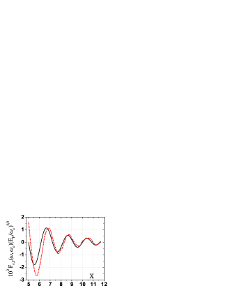
Figure 3: (Color online) Interaction-induced contribution to the ac conductivity calculated numerically from Eq. (Magneto-oscillations due to electron-electron interactions in the ac conductivity of a 2D electron gas) (dotted line) and from asymptotic expression Eq. (Magneto-oscillations due to electron-electron interactions in the ac conductivity of a 2D electron gas) (full line) are plotted vs dimensionless frequency $x=2^{1/3}\omega/(E_{\mbox{\tiny F}}^{1/3}\omega_{c}^{2/3})=3(z/4)^{2/3}$. The calculations are performed for dimensionless disorder $1/(E_{\mbox{\tiny F}}\tau)=0.08(\omega_{c}/E_{\mbox{\tiny F}})^{2/3}$ and dimensionless temperature $T/E_{\mbox{\tiny F}}=0.06(\omega_{c}/E_{\mbox{\tiny F}})^{2/3}$.

The above derivation suggests that oscillatory behavior of the correction Eq. (Magneto-oscillations due to electron-electron interactions in the ac conductivity of a 2D electron gas) establishes only at large $z\gg 1$, which corresponds to the nodes of $\cos(z-\pi/4)$ with high numbers. To find out where the asymptotics Eq. (Magneto-oscillations due to electron-electron interactions in the ac conductivity of a 2D electron gas) actually applies, we have evaluated the double integral Eq. (Magneto-oscillations due to electron-electron interactions in the ac conductivity of a 2D electron gas) numerically. The result is plotted in Fig. 3 and indicates that Eq. (Magneto-oscillations due to electron-electron interactions in the ac conductivity of a 2D electron gas) applies starting already from the third node.

Other diagrams. Contribution Eq. (Magneto-oscillations due to electron-electron interactions in the ac conductivity of a 2D electron gas) to $\delta\sigma^{int}(\omega)$ is the result of calculation of a single diagram $a$ in Fig.  2. Other diagrams, involving two electron-electron scattering processes and yielding contributions with a structure similar to Eq. (Magneto-oscillations due to electron-electron interactions in the ac conductivity of a 2D electron gas), are shown in Fig. 2. Diagrams $b$, $c$, and $d$ are captured within the self-consistent Born approximation, and correspond to certain terms in $\delta\Sigma^{int}$, see c) in Fig. 2 (inset). Diagrams $e$-$h$ in Fig. 2 are of the same order as $a$-$d$, but they are not contained in Eq. (Magneto-oscillations due to electron-electron interactions in the ac conductivity of a 2D electron gas); these diagrams emerge from the general expression Eq. (4) for $\sigma(\omega)$. Taking all the diagrams into account leads to the modification of the function $D(z)$ from $z^{-5/6}$ to ${\tilde{D}}(z)=-32z^{-5/6}+64z^{1/6}$, where the factors $-32$ and $64$ account for the spin indices and for the number of closed fermion loops in different diagrams. The second term, $\propto z^{1/6}$, arises from the diagrams $b$, $e$ and $d$, $h$ in Fig. 2. Since the oscillations in Eq. (Magneto-oscillations due to electron-electron interactions in the ac conductivity of a 2D electron gas) develop at $z\gg 1$, these diagrams are, actually, dominant.

Numerical estimates. Note that, in terms of $B$-periodicity, oscillations Eq. (Magneto-oscillations due to electron-electron interactions in the ac conductivity of a 2D electron gas) coincide with oscillations Eq. (1) upon rescaling $\omega_{c}$ by $2\pi/C_{\omega}$ in the argument of cosine, and by $2\pi/3C_{\omega}$ in the Dingle factor. For a typical ac frequency $\hbar\omega\sim 3$K and density $n\sim 10^{11}$cm^-2 in the experiments zudov01 ; zudov03 ; mani02 ; dorozhkin03 ; studenikin ; vitkalov this shifts the domain of oscillations Eq. (Magneto-oscillations due to electron-electron interactions in the ac conductivity of a 2D electron gas) from $B\sim 0.2$T to $B\lesssim 10^{-2}$T. For such $B$ the observation of the oscillations requires $T<\omega_{c}/6\pi C_{\omega}\sim 20$mK, which was not the case in Refs. zudov01, ; zudov03, ; mani02, ; dorozhkin03, ; studenikin, ; vitkalov, . For observation of magneto-oscillations Eq. (Magneto-oscillations due to electron-electron interactions in the ac conductivity of a 2D electron gas) higher densities $n\sim 5\cdot 10^{11}$cm^-2 and frequencies $\hbar\omega\sim 15$K are needed.

References

- (1) J. P. Kotthaus, G. Abstreiter, and J. F. Koch, Solid State Commun. 15, 517 (1974).
- (2) M. A. Zudov, et al., Phys. Rev. B 64, 201311 (2001).
- (3) M. A. Zudov, et al., Phys. Rev. Lett. 90, 046807 (2003).
- (4) R. G. Mani, et al., Nature (London) 420, 646 (2002).
- (5) S. I. Dorozhkin, JETP Lett. 77, 577 (2003).
- (6) I. A. Dmitriev, A. D. Mirlin, and D. G. Polyakov, Phys. Rev. Lett. 91, 226802 (2003).
- (7) I. A. Dmitriev, A. D. Mirlin, and D. G. Polyakov, Phys. Rev. B 70, 165305 (2004).
- (8) M. G. Vavilov and I. L. Aleiner, Phys. Rev. B 69, 035303 (2004).
- (9) I. A. Dmitriev, et al., Phys. Rev. B 71, 115316 (2005).
- (10) I. A. Dmitriev, A. D. Mirlin, and D. G. Polyakov, Phys. Rev. B 75, 245320 (2007).
- (11) A. Gold and V. T. Dolgopolov, Phys. Rev. B 33, 1076 (1986).
- (12) G. Zala, B. N. Narozhny, and I. L. Aleiner, Phys. Rev. B 64, 214204 (2001).
- (13) I. V. Gornyi and A. D. Mirlin, Phys. Rev. B 69, 045313 (2004).
- (14) A. M. Rudin, I. L. Aleiner, and L. I. Glazman, Phys. Rev. B 55, 9322 (1997).
- (15) For the same reason we neglect the Zeeman splitting
- (16) A. V. Chubukov and D. L. Maslov, Phys. Rev. B 68, 155113 (2003); ibid. 69, 121102 (2004).
- (17) T. A. Sedrakyan, E. G. Mishchenko, and M. E. Raikh, Phys. Rev. Lett. 99, 036401 (2007).
- (18) L. P. Gor’kov, Sov. Phys. JETP, 9, 1364 (1959).
- (19) S. A. Studenikin, et al., Solid State Commun, 129, 341 (2004).
- (20) A. A. Bykov, et al., preprint cond-mat/0603398.