Effect of the Spatial Dispersion on the Shape of a Light Pulse in a Quantum Well

Abstract

Reflectance, transmittance and absorbance of a symmetric light pulse, the carrying frequency of which is close to the frequency of interband transitions in a quantum well, are calculated. Energy levels of the quantum well are assumed discrete, and two closely located excited levels are taken into account. A wide quantum well (the width of which is comparable to the length of the light wave, corresponding to the pulse carrying frequency) is considered, and the dependance of the interband matrix element of the momentum operator on the light wave vector is taken into account. Refractive indices of barriers and quantum well are assumed equal each other. The problem is solved for an arbitrary ratio of radiative and nonradiative lifetimes of electronic excitations. It is shown that the spatial dispersion essentially affects the shapes of reflected and transmitted pulses. The largest changes occur when the radiative broadening is close to the difference of frequencies of interband transitions taken into account.

Irradiation of the low-dimensional semiconductor systems by light pulses and analysis of reflected and transmitted pulses allow to obtain the information regarding the structure of energy levels as well as relaxation processes.

The radiative mechanism of relaxation of excited energy levels in quantum wells arises due to a violation of the translation symmetry perpendicular to the he quantum well plane bb1 ; bb2 . At low temperatures, low impurity doping and perfect boundaries of quantum wells, the contributions of the radiative and nonradiative relaxation can be comparable. In such situation, one cannot be limited by the linear approximation on the electron - light interaction. All the orders of the interaction have to be taken into account bb3 ; bb4 ; bb5 ; bb6 ; bb7 ; bb8 ; bb9 . Alterations of asymmetrical bb10 ; bb11 ; bb12 ; bb13 and symmetrical bb13 ; bb14 ; bb15 light pulses are valid for narrow quantum wells under conditions $k\,d\ll\,1$ ($d$ is the quantum well width, $k$ is the magnitude of the light wave vector corresponding to the carrying frequency of the light pulse) and an independence of optical characteristics of a quantum well on $d$. However, a situation is possible when the size quantization is preserved and for wide quantum wells if $k\,d\geq\,1$ (see corresponding estimates in bb16 ). In such a case, we have to take into account the spatial dispersion of a monochromatic wave bb9 ; bb19 and waves composing the light pulse bb16 .

Our investigation is devoted to the influence of the spatial dispersion on the optical characteristics (reflectance, transmittance and absorbance) of a quantum well irradiated by the symmetric light pulse. A system, consisting of a deep quantum well of type I, situated inside of the space interval $0\leq z\leq d$, and two semi-infinite barriers, is considered. A constant quantizing magnetic field is directed perpendicular to the quantum well plane what provides the discrete energy levels of the electron system. A stimulating light pulse propagates along the $z$ axis from the side of negative values $z$. The barriers are transparent for the light pulse which is absorbed in the quantum well to initiate the direct interband transitions. The intrinsic semiconductor and zero temperature are assumed.

The final results for two closely spaced energy levels of the electronic system in a quantum well are obtained. Effect of other levels on the optical characteristics may be neglected, if the carrying frequency $\omega_{\,\ell}$ of the light pulse is close to the frequencies $\omega_{\,1}$ and $\omega_{\,2}$ of the doublet levels, and other energy levels are fairly distant. It is assumed that the doublet is situated near the minimum of the conduction band, the energy levels may be considered in the effective mass approximation, and the barriers are infinitely high.

In the case $\hbar\,K_{\perp}=0$ ($\hbar\,K_{\perp}$ is the vector of the quasi-momentum of electron-hole pair in the quantum well plane) in a quantum well, the discrete energy levels are the excitonic energy levels in a zero magnetic field or energy levels in a quantizing magnetic field directed perpendicularly to the quantum well plane. As an example, the energy level of the electron-hole pair in a quantizing magnetic field directed along the $z$ axis (without taking into account the Coulomb interaction between the electron and hole which is a weak perturbation for the strong magnetic fields and not too wide quantum wells) is considered.

I The electric field

Let us consider a situation when a symmetric exciting light pulse propagates through a single quantum well along the $z$ axis from the side of negative values of $z$. Analogously to bb13 ; bb14 ; bb15 , the electric field is chosen as

$${\bf E}_{\,0}\,(z,t)={\bf e}_{\,\ell\,}E_{\,0\,}e^{-i\omega_{\,\ell\,}p}$$

$$\times\left\{\Theta(p)e^{-\gamma_{\,\ell\,}p/2}\,+\,[1-\Theta(p)]e^{\gamma_{\,\ell\,}p/2}\right\}+c.c.,$$ (1)

where $E_{\,0}$ is the real amplitude, $p=t-\nu\,z/\,c$,

$${\bf e}_{\,\ell}={1\over\sqrt{2}}({\bf e}_{\,x}\,\pm\,i\,{\bf e}_{\,y})$$

are the unite vectors of the circular polarization, ${\bf e}_{\,x}$ ${\bf e}_{\,y}$ are the real unite vectors, $\Theta(p)$ is the Heaviside function, $1/\gamma_{\,\ell}$ determines the pulse width, $c$ is the light velocity in vacuum, $\nu$ is the refraction index, which is assumed the same for the quantum well and barriers (the approximation of a homogeneous media). The Fourier-transform of (I) is as follows

$${\bf E}_{\,0}(z,\omega)\,=\,e^{ikz}\left[{\bf e}_{\,\ell}\,E_{\,0}(\omega)+{\bf e}_{\,\ell}^{*}\,E_{\,0}(-\omega)\right],$$

$$E_{\,0}(\omega)\,=\,\frac{E_{\,0}\,\gamma_{\,\ell}}{(\omega-\omega_{\,\ell})^{2}+(\gamma_{\,\ell}/2)^{2}},~{}~{}~{}~{}k\,=\,\frac{\nu\omega}{c}.$$ (2)

The electric field in the region $z\leq 0$ consists of the sum of the exciting and reflected pulses. The Fourier-transform may be written as

$${\bf E}^{\,\ell}\,(z,\omega)\,=\,{\bf E}_{\,0}\,(z,\omega)\,+\,\Delta{\bf E}^{\,\ell}\,(z,\omega),$$

where $\Delta{\bf E}^{\,\ell}(z,\omega)$ is the electric field of the reflected pulse

$$\Delta{\bf E}^{\,\ell}(z,\omega)\,=\,{\bf e}_{\,\ell}\,\Delta E^{\,\ell}(z,\omega)\,+\,{\bf e}_{\,\ell}^{\,*\,}\,\Delta E^{\,\ell}(z,-\omega).$$ (3)

In the region $z\geq d$, there is only the transmitted pulse, and its electric field is

$${\bf E}^{\,r}(z,\omega)\,=\,{\bf e}_{\,\ell}\,E^{\,r}(z,\omega)\,+\,{\bf e}_{\,\ell}^{\,*\,}\,E^{\,r}(z,-\omega).$$ (4)

It is assumed below that the pulse, having absorbed in the quantum well, stimulates the interband transitions and, consequently, the appearance of a current. In barriers, the absorption is absent. Therefore, for the complex amplitudes $\Delta E^{\,\ell}(z,\omega)$ and $E^{\,r}(z,\omega)$ in barriers for $z\leq 0$ and $z\geq d$, we obtain the expression

$$\frac{d^{\,2}E}{d\,z^{\,2}}\,+\,k^{\,2}\,E\,=\,0.$$ (5)

The expression for the electric field inside of the quantum well $(0\leq z\leq d)$ has a form

$$\frac{d^{\,2}E}{d\,z^{\,2}}\,+\,k^{\,2}\,E\,=\,-\frac{4\pi i\,\omega}{c^{\,2}}\,J(z,\omega),$$ (6)

where $J(z,\omega)$ is the Fourier-transform of the current density, averaged on the ground state of the system. The current is induced by the monochromatic wave of the frequency $\omega$. In the case of two excited energy levels, $J(z,\omega)$ is expressed as follows

$$J(z,\omega)\,=\,\frac{i\nu c}{4\pi}\sum_{j=1}^{2}\,\frac{\gamma_{\,rj}\,\Phi_{\,j}(z)}{\tilde{\omega}_{\,j}}\int_{0}^{d}\,dz^{\prime}\,\Phi_{\,j}(z^{\prime})\,E(z^{\,\prime},\omega),$$ (7)

$$\tilde{\omega}_{\,j}\,=\,\omega\,-\,\omega_{\,j}\,+\,i\gamma_{\,j}/2.$$ (8)

where $\gamma_{\,j}$ is the nonradiative damping of the doublet, $\gamma_{\,r\,j}$ is the radiative damping of the levels of the doublet in the case of narrow quantum wells, when the spatial dispersion of electromagnetic waves may be neglected.

In particular, the doublet system may be represented by a magnetopolaron state bb18 . In such a case,

$$\gamma_{\,r,j}\,=\,\gamma_{\,r}\,Q_{\,j},~{}~{}~{}~{}~{}~{}\gamma_{\,r}\,=\,\frac{2e^{2}}{\hbar\,c\nu}\,\frac{p^{\,2}_{\,c\,v}}{\hbar\,\omega_{\,g}\,m_{\,0}}\,\frac{|e|H}{m_{\,0}\,c},$$

where $m_{\,0}$ is the free electron mass, $H$ is the magnetic field, $e$ is the electron charge, $p_{\,c\,v\,}$ is the matrix element of the momentum, corresponding to the circular polarization, $p_{\,c\,v\,}^{2}=|p_{\,c\,v\,x\,}|^{2}+|p_{\,c\,v\,y\,}|^{2}$. The factor

$$Q_{\,j}={1\over 2}\pm{\hbar\,(\Omega_{\,c}-\omega_{\,LO})\over 2\sqrt{\hbar^{2}(\Omega_{\,c}-\omega_{\,LO})^{2}+(\Delta E_{\,pol})^{2}}}$$

determines the change of the radiative timelife at a deflection of the magnetic field from the resonant value when the resonant condition $\Omega_{\,c}\,=\,\omega_{\,LO}$ is carried out. $\Delta E_{\,pol}$ is the polaron splitting, $\Omega_{\,c}$ and $\omega_{\,LO}$ are the cyclotron frequency and optical phonon frequency, respectively. In the resonance, $Q_{\,j}=1/2$ and $\gamma_{\,r1}\,=\,\gamma_{\,r2}$.

When calculating $J(z,\omega)$, it was assumed that the Lorentz force, determined by the external magnetic field, is large in comparison with the Coulomb and exchange forces in the electron-hole pair. In that case, the variables $z$ (along magnetic field) and ${\bf r}_{\perp}$ (in the quantum well plane) in the wave function of the electron-hole pair may be separated. This condition is carried out for the quantum well on basis of GaAs for the magnetic field, corresponding to the magnetopolaron formation bb9 . Besides, if the energy of the size quantization exceeds the Coulomb and exchange energies, the electron-hole pair may be considered as a free particle. Then, in the approximation of the effective mass and infinitely high barriers, the wave function, describing the dependence on $z$ , accepts a simple form

$$\Phi_{\,j}(z)={2\over d}\,sin{\pi m_{\,c}z\over d}\,sin{\pi m_{\,v}z\over d},~{}~{}0\leq z\leq d,$$ (9)

and $\Phi_{\,j}(z)\,=\,0$ in barriers, where $m_{\,c}\,(m_{\,v})$ are the quantum numbers of the size-quantization of an electron (hole).

In the real systems, the approximation (9) is not always carried out. However, the taking into account the Coulomb and exchange interactions will result only into some changes of the function $\Phi_{\,j}(z)$, what does not change qualitatively the optical characteristics, as it was shown for the monochromatic irradiation bb20 .

Indices $j=1$ and $j=2$ in $\Phi_{\,j}(z)$ correspond to the pairs of quantum numbers of the size-quantization in a direct interband transition. $m^{(1)}_{\,c\,(\,v)}$ corresponds to the index $j=1$, and $m^{(2)}_{\,c\,(\,v)}$ corresponds to the index $j=2$. In interband transitions, the Landau quantum numbers are conserved. The total electric field $E$ is included into the RHS of (7), what is connected with the refuse from the perturbation theory on the coupling constant $e^{2}/\hbar c$.

In further calculations, an equality of quantum numbers $m^{(1)}_{\,c\,v}\,=\,m^{(2)}_{\,c\,v}$ is assumed. Then,

$$\Phi_{\,1}(z)\,=\,\Phi_{\,2}(z)\,=\,\Phi(z),$$

and the current density in the RHS of (7) takes the form

$$J(z,\omega)\,=\,\frac{i\,\nu\,c}{4\,\pi}\bigg{(}\frac{\gamma_{\,r1}}{{\omega}\,-\,\omega_{\,1}\,+\,i\gamma_{\,1}}+\frac{\gamma_{\,r2}}{{\omega}-\,\omega_{\,2}\,+\,i\gamma_{\,2}}\bigg{)}$$

$$\times\Phi(z)\int_{0}^{d}dz^{\prime}\Phi(z^{\prime})E(z^{\prime}).$$ (10)

With the help of the indicated simplifications, as it was shown in bb9 ; bb18 ; bb20 , the field amplitudes in the Fourier-representation $\Delta E^{\,\ell}(z,\omega)$ and $E^{\,r}(z,\omega)$ result in

$$\Delta E^{\,\ell}(z,\omega)\,=\,-iE_{0}(\omega)(-1)^{m_{\,c}+m_{\,v}}e^{-ik(z-d)}{\cal N},$$

$$E^{\,r}(z,\omega)\,=\,E_{0}(\omega)e^{ikz}(1-i{\cal N}),$$ (11)

where $E_{0}(\omega)$ is given in (3). Here, the frequency dependence is determined by the function

$${\cal N}\,=\,\frac{\varepsilon\,(\gamma_{\,r1}\,\tilde{\omega}_{2}\,+\,\gamma_{\,r2}\,\tilde{\omega}_{1})/2}{\tilde{\omega}_{1}\,\tilde{\omega}_{2}\,+\,i\varepsilon(\gamma_{\,r1}\,\tilde{\omega}_{2}\,+\,\gamma_{\,r2}\,\tilde{\omega}_{1})/2}.$$ (12)

The function ${\cal N}$ includes the value

$$\varepsilon\,=\,\varepsilon^{\prime}\,+\,i\varepsilon^{\prime\prime},$$ (13)

which determines influence of the spatial dispersion on the radiative broadening ($\varepsilon^{\prime}\,\gamma_{\,r}$) and shift ($\varepsilon^{\prime\prime}\,\gamma_{\,r}$) of the doublet levels. $\varepsilon^{\prime}$ and $\varepsilon^{\prime\prime}$ are equal bb9 ; bb20 :

$$\varepsilon^{\prime}\,=\,Re\,\varepsilon\,=\,2{\cal B}^{2}\,\big{[}1-(-1)^{m_{\,c}+m_{\,v}}\cos kd\,\big{]},$$ (14)

$$\varepsilon^{\prime\prime}=Im\varepsilon=2{\cal B}$$

$$\times\Bigg{(}\frac{(1+\delta_{m_{c},m_{v}})(m_{c}+m_{v})^{2}+(m_{c}-m_{v})^{2}}{8m_{c}m_{v}}$$

$$-(-1)^{m_{c}+m_{v}}{\cal B}\sin kd-\frac{(2+\delta_{m_{c},m_{v}})(kd)^{2}}{8\pi^{2}m_{c}m_{v}}\Bigg{)},$$ (15)

$${\cal B}\,=\,\frac{4\pi^{\,2}\,m_{\,c}\,m_{\,v}\,kd}{[\pi^{\,2}\,(m_{\,c}+m_{\,v})^{2}-(kd)^{2}\,]\,[(kd)^{2}\,-\pi^{\,2}\,(m_{\,c}-m_{\,v})^{2}\,]}$$

(if $kd\to 0$, $\varepsilon\to 1\,(m_{\,c}\,=\,m_{\,v}$, an allowed transition ) and $\varepsilon\to 0\,(m_{\,c}\,\neq\,m_{\,v}$, a forbidden transition)).

II The time-dependence of the electric field of reflected and transmitted light pulses

With the help of the standard formulas, let us go to the time-representation

$$\Delta E^{\,\ell}(z,t)\,\equiv\,\Delta E^{\,\ell}(s)\,=$$

$$=\frac{1}{2\pi}\int_{-\infty}^{+\infty}d\omega\,e^{-i\omega\,s}\,\Delta E^{\,\ell}(z,\omega),~{}~{}s=t+\nu z/c,~{}~{}~{}~{}~{}$$ (16)

$$E^{\,r}(z,t)\,\equiv\,E^{\,r}(p)\,=\,\frac{1}{2\pi}\int_{-\infty}^{+\infty}d\omega\,e^{-i\omega\,p}\,E^{\,r}(z,\omega),$$

$$p=t-\nu z/c.$$ (17)

The vectors $\Delta{\bf E}^{\,\ell}(s)$ and ${\bf E}^{\,r}(p)$ have the form

$$\Delta{\bf E}^{\,\ell}(s)\,=\,{\bf e}_{\,\ell}\,\Delta E^{\,\ell}(s)+c.c.,$$

$${\bf E}^{\,r}(p)\,=\,{\bf e}_{\,\ell}\,E^{\,r}(p)+c.c..$$ (18)

It is seen from expressions $(\ref{eq11})$ and $(\ref{eq12})$ that the denominator in integrands of $(\ref{eq16})$ and $(\ref{eq17})$ is the same. It may be transformed conveniently to the form

$$\tilde{\omega}_{1}\,\tilde{\omega}_{2}\,+\,i(\varepsilon/2)\,(\gamma_{\,r1}\,\tilde{\omega}_{2}\,+\,\gamma_{\,r2}\,\tilde{\omega}_{1})$$

$$=(\omega-\Omega_{\,1})\,(\omega-\Omega_{\,2}),$$ (19)

where $\Omega_{\,1}$ and $\Omega_{\,2}$ determine the poles of the integrand in the complex plane $\omega$. They are equal

$$\Omega_{1,2}=\frac{1}{2}\Bigg{\{}\omega_{1}+\omega_{2}-\frac{i}{2}(\gamma_{1}+\gamma_{2})-\frac{i\varepsilon}{2}(\gamma_{r1}+\gamma_{r2})$$

$$\pm\Big{(}[\omega_{1}-\omega_{2}-{i\over 2}(\gamma_{1}-\gamma_{2})-{i\varepsilon\over 2}(\gamma_{r1}-\gamma_{r2})]^{2}$$

$$-\varepsilon^{2}\gamma_{r1}\gamma_{r2}\Big{)}^{1/2}\Bigg{\}}.$$ (20)

Thus, in the integrands of II) and (II), there are 4 poles: $\omega\,=\,\omega_{\,\ell}\pm i\gamma_{\,\ell}/2$ and $\omega=\Omega_{\,1,2}$. The pole $\omega\,=\,\omega_{\,\ell}+i\gamma_{\,\ell}/2$ is situated in the upper half plane, others are situated in the lower half plane.

Integrating in the complex plane $\omega$, we obtain that the function $\Delta E^{\,\ell}(z,t)$, determining, according to (II), the electric field vector of the reflected pulse $\Delta{\bf E}^{\,\ell}(z,t)$, has the form

$$\Delta E^{\,\ell}(z,t)\,=\,-iE_{\,0}(-1)^{m_{\,c}+m_{\,v}}e^{ikd}$$

$$\times\{R_{1}[1-\Theta(s)]+(R_{2}+R_{3}+R_{4})\Theta(s)\},$$ (21)

where

$$R_{1}\,=\,\exp(-i\omega_{\,\ell}s+\gamma_{\,\ell}s/2)$$

$$\times\Bigg{(}\frac{\bar{\gamma}_{\,r1}/2}{\omega_{\,\ell}-\Omega_{1}+i\gamma_{\,\ell}/2}+\frac{\bar{\gamma}_{\,r2}/2}{\omega_{\,\ell}-\Omega_{2}+i\gamma_{\,\ell}/2}\Bigg{)},$$

$$R_{2}\,=\,\exp(-i\omega_{\,\ell}-\gamma_{\,\ell}s/2)$$

$$\times\Bigg{(}\frac{\bar{\gamma}_{\,r1}/2}{\omega_{\,\ell}-\Omega_{1}-i\gamma_{\,\ell}/2}+\frac{\bar{\gamma}_{\,r2}/2}{\omega_{\,\ell}-\Omega_{2}-i\gamma_{\,\ell}/2}\Bigg{)},$$

$$R_{3}\,=\,-\exp(-i\Omega_{1}s)(\bar{\gamma}_{\,r1}/2)$$

$$\times\Bigg{(}\frac{1}{\omega_{\,\ell}-\Omega_{1}-i\gamma_{\,\ell}/2}-\frac{1}{\omega_{\,\ell}-\Omega_{1}+i\gamma_{\,\ell}/2}\Bigg{)},$$

$$R_{4}\,=\,-\exp(-i\Omega_{2}s)(\bar{\gamma}_{\,r2}/2)$$

$$\times\Bigg{(}\frac{1}{\omega_{\,\ell}-\Omega_{2}-i\gamma_{\,\ell}/2}-\frac{1}{\omega_{\,\ell}-\Omega_{2}+i\gamma_{\,\ell}/2}\Bigg{)},$$ (22)

where

$$\bar{\gamma}_{\,r1}\,=\,\varepsilon^{\prime}\,\gamma_{\,r1}\,+\Delta\gamma,\bar{\gamma}_{\,r2}\,=\,\varepsilon^{\prime}\,\gamma_{\,r2}\,-\Delta\gamma,$$

$$\Delta\gamma\,=\,\frac{\varepsilon^{\prime}\,\gamma_{\,r1}(\Omega_{2}-\omega_{2}+i\gamma_{2}/2)}{\Omega_{1}-\Omega_{2}}$$

$$+\frac{\varepsilon^{\prime}\,\gamma_{\,r2}(\Omega_{1}-\omega_{1}+i\gamma_{1}/2)}{\Omega_{1}-\Omega_{2}}.$$ (23)

The function $E^{\,r}(z,t)$, corresponding to a transmitted light pulse, is represented in the form

$$E^{\,r}(z,t)\,=E_{\,0}{T_{1}[1-\Theta(p)]+(T_{2}+T_{3}+T_{4})\Theta(p)\over\Omega_{1}-\Omega_{2}},$$ (24)

where

$$T_{1}\,=\,\exp(-i\omega_{\,\ell}p+\gamma_{\,\ell}p/2)M(\omega_{\,\ell}+i\gamma_{\,\ell}/2)$$

$$\times\Bigg{(}\frac{1}{\omega_{\,\ell}-\Omega_{1}+i\gamma_{\,\ell}/2}-\frac{1}{\omega_{\,\ell}-\Omega_{2}+i\gamma_{\,\ell}/2}\Bigg{)},$$

$$T_{2}\,=\,\exp(-i\omega_{\,\ell}p-\gamma_{\,\ell}p/2)M(\omega_{\,\ell}-i\gamma_{\,\ell}/2)$$

$$\times\Bigg{(}\frac{1}{\omega_{\,\ell}-\Omega_{1}-i\gamma_{\,\ell}/2}-\frac{1}{\omega_{\,\ell}-\Omega_{2}-i\gamma_{\,\ell}/2}\Bigg{)},$$

$$T_{3}\,=\,-\exp(-i\Omega_{1}\,p)M(\Omega_{1})$$

$$\times\Bigg{(}\frac{1}{\omega_{\,\ell}-\Omega_{1}-i\gamma_{\,\ell}/2}-\frac{1}{\omega_{\,\ell}-\Omega_{1}+i\gamma_{\,\ell}/2}\Bigg{)},$$

$$T_{4}\,=\,\exp(-i\Omega_{2}\,p)M(\Omega_{2})$$

$$\times\Bigg{(}\frac{1}{\omega_{\,\ell}-\Omega_{2}-i\gamma_{\,\ell}/2}-\frac{1}{\omega_{\,\ell}-\Omega_{1}+\gamma_{\,\ell}/2}\Bigg{)}.$$ (25)

The function $M$ has the structure

$$M(\omega)=(\omega-\omega_{1}+i\gamma_{1}/2)(\omega-\omega_{2}+i\gamma_{2}/2)-$$

$$(\varepsilon^{\prime\prime}/2)[\gamma_{r1}(\omega-\omega_{2}+i\gamma_{2}/2)+\gamma_{r2}(\omega-\omega_{1}+i\gamma_{1}/2)].$$

When the electric field of stimulating light pulse ${\bf E}^{\,0}(z,t)$ (determined in (I)) is extracted from ${\bf E}^{\,r}(z,t)$ , i.e., it is assumed

$${\bf E}^{\,r}(z,t)\,=\,{\bf E}^{\,0}(z,t)+\Delta{\bf E}^{\,r}(z,t),$$ (26)

then, $\Delta{\bf E}^{\,r}(z,t)$ will differ from $\Delta{\bf E}^{\,\ell}(z,t)$ only by substitution of the variable $s=t+\nu z/c$ by $p=t-\nu z/c$ and by absence of the factor $(-1)^{m_{\,c}+m_{\,v}}\exp(ikd)$.

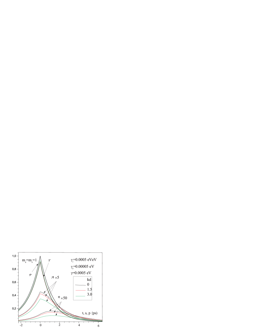
Figure 1: The reflectance ${\cal R}$, transmittance ${\cal T}$, absorbance ${\cal A}$, and stimulating pulse ${\cal P}$ as time dependent functions for three magnitudes of the parameter $kd$ in the case of a long stimulating pulse $(\gamma_{\,\ell\,}\ll\Delta\omega)$ $\gamma_{\,r}\ll\gamma,\gamma_{\,\ell\,}.\,\Delta\omega=6.65.10^{-3}eV,\,\omega_{\,\ell\,}=Re\,\Omega_{1}=\Omega_{\,res}.$

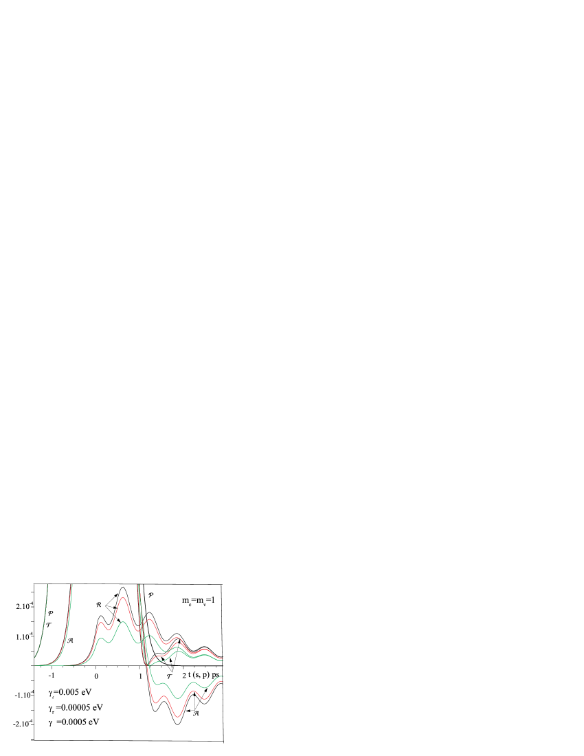
Figure 2: Same as in Fig.1 for an exciting pulse of a middle duration $(\gamma_{\,\ell\,}\simeq\Delta\omega)$ $\gamma_{\,r}\ll\gamma\ll\gamma_{\,\ell\,}.$

Thus, being taken into account, the spatial dispersion provides a renormalization of radiative damping $\gamma_{\,r\,i}$. In nominators of formulas (II), the renormalization leads to multiplication of $\gamma_{\,r\,i}$ on the real factor $\varepsilon^{\prime}$, i.e., decreases the value $\gamma_{\,r\,i}$ (diagrams of functions $\varepsilon^{\prime}$ and $\varepsilon^{\prime\prime}$ are represented in bb9 ). In denominators, $\gamma_{\,r\,i}$ is multiplied on the complex function $\varepsilon$, that means the appearance, together with the change of the radiative broadening, of a shift of resonant frequencies. In the limit $kd=0$, expressions (II) - (II) coincide with obtained in (14).

III The reflectance, transmittance and absorbance of stimulating light pulse

The energy flux ${\bf S}(p)$, corresponding to the electric field of stimulating light pulse, is equal

$${\bf S}(p)\,=\frac{\mathbf{e_{z}}}{4\pi}\frac{c}{\nu}({\bf E}^{\,0}(z,t))^{2}\,=\,{\bf e}_{z}S_{0}{\cal P}(p),$$ (27)

where $S_{0}=cE_{0}^{2}/2\pi\nu,{\bf e}_{z}$ is the unite vector along the light pulse. The dimensionless function

$${\cal P}(p)={({\bf E}^{\,0}(z,t))^{2}\over S_{0}}=\Theta(p)e^{-\gamma_{\ell}p}+[1-\Theta(p)]e^{\gamma_{\ell}p}$$ (28)

determines the spatial and time dependence of the energy flux of stimulating pulse. The flux, transmitted through the quantum well, has a form

$${\bf S}^{r}\,={{\bf e}_{z}c\over 4\pi\nu}({\bf E}^{\,r}(z,t))^{2}\,=\,{\bf e}_{z}S_{0}{\cal T}(p),$$ (29)

the reflected energy flux has a form

$${\bf S}^{\,\ell}\,=-{{\bf e}_{z}c\over 4\pi\nu}({\bf E}^{\,\ell}(z,t))^{2}\,=\,-{\bf e}_{z}S_{0}{\cal R}(s).$$ (30)

The dimensionless functions ${\cal T}(p)$ and ${\cal R}(s)$ correspond to parts of transmitted and reflected energy fluxes of the stimulating pulse. The dimensionless absorbance is defined as

$${\cal A}(p)\,=\,{\cal P}(p)-{\cal R}(p)-{\cal T}(p)$$ (31)

(since for reflection $z\leq 0$, the variable in ${\cal R}$ is $s=t-|z|/c$).

The dependencies of the reflectance ${\cal R}$, transmittance ${\cal T}$, absorbance ${\cal A}$, and stimulated momentum ${\cal P}$ on the variable $p$ (or $s$ for ${\cal R}$) for the case $m_{\,c\,}=m_{\,v\,}=1$ are represented in figures. It was assumed also that

$$\gamma_{\,r\,1}\,=\,\gamma_{\,r\,2}\,=\,\gamma_{\,r},~{}~{}~{}~{}\gamma_{\,1}=\gamma_{\,2}=\gamma.$$ (32)

It follows from (II) and (24) that the resonant frequencies are $\omega_{\,\ell}=Re\,\Omega_{1}$ and $\omega_{\,\ell}=Re\,\Omega_{2}$. The calculations were performed for

$$\omega_{\,\ell}\,=\,Re\,\Omega_{1}\,=\,\Omega_{res}.$$ (33)

Let us go from the frequency $\omega_{\,\ell}$ to

$$\Omega\,=\,\omega_{\,\ell}-\omega_{1},$$ (34)

then the resonant frequency is

$$\Omega_{res}\,=\,\frac{1}{2}\big{[}-\Delta\omega+\varepsilon^{\prime}\gamma_{\,r}+Re\,\sqrt{(\Delta\omega)^{2}-\varepsilon^{2}\gamma_{\,r}^{2}}\,\big{]}.$$ (35)

It depends on three parameters: $\Delta\omega=\omega_{1}-\omega_{2},\gamma_{\,r}$ and $kd$, since the complex function $\varepsilon$ depends on $kd$ (see (I)).

Functions ${\cal R},{\cal T},{\cal A}$ and ${\cal P}$ are homogeneous functions of the inverse lifetimes and frequencies $\omega_{1},\omega_{2},\omega_{\,\ell}$. Therefore, a choice of the measurement units is arbitrary. For the sake of certainty, all these values are expressed in $eV$. The time dependence of the optical characteristics of a quantum well is represented in figures for the different magnitudes of $kd$. The curves, corresponding to $kd=0$, were obtained in bb14 . It was assumed in calculations that $\Delta\omega=0.065eV$, what corresponds to the magnetopolaron state in a quantum well on basis of GaAs and to the width $d=300\AA$ of the quantum well bb18 ; bb19 ; bb21 .

IV The Discussion of results

Fig.1 corresponds to a long (wide in comparison to $\Delta\omega$) stimulating pulse and a small radiative broadening $(\gamma_{\,r}\ll\gamma,\gamma_{\,\ell})$. In this case, the transmittance ${\cal T}$ dominates. The shape of the curve weakly differs from ${\cal P}$ and weakly depends on $kd$. The dependence on the spatial dispersion is seen at the curves ${\cal R}$ and ${\cal A}$. For example, the reflectance ${\cal R}$ at $kd=3$ is two times less than at $kd=0$. However, the magnitude ${\cal R}$ is shares of percent.

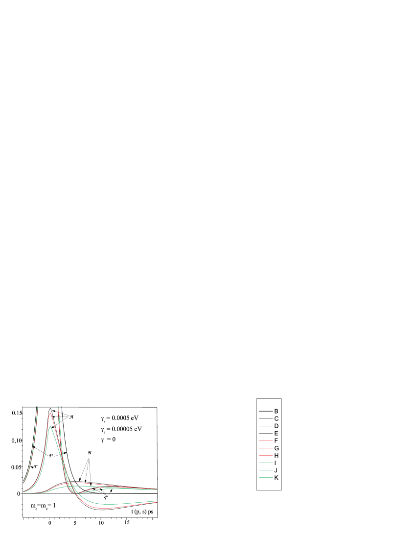
Figure 3: Same as in Fig.1 for an exciting pulse of a middle duration $(\gamma_{\,\ell\,}\simeq\Delta\omega)$ $\gamma_{\,r}\ll\gamma\ll\gamma_{\,\ell\,}.$

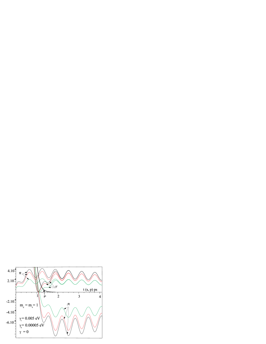
Figure 4: Same as in Fig.1 for an exciting pulse of a middle duration $(\gamma_{\,\ell\,}\simeq\Delta\omega)$ $\gamma=0.$

Fig.2 corresponds to a stimulating light pulse of a middle length, when $\gamma_{\,\ell}\simeq\Delta\omega$ and $\gamma_{\,r}\ll\gamma\ll\gamma_{\,\ell}$. There appear peculiarities: a light generation (negative absorption) after the light pulse transmission and oscillations of ${\cal R},{\cal A}$ and ${\cal T}$. The generation is a consequence of the fact that the electronic system has no time to irradiate the energy during the propagation of such pulse. Oscillations is a consequence of beatings with the frequency (under condition $\omega_{\,\ell}=Re\,\Omega_{1}$)

$$Re\,(\Omega_{1}\,-\,\Omega_{2})\,=\,Re\,\sqrt{(\omega_{1}-\omega_{2})^{2}-(\varepsilon^{\prime}+i\varepsilon^{\prime\prime})^{2}\gamma_{\,r}^{2}}.$$ (36)

A noticeable effect of the spatial dispersion takes place in the reflectance ${\cal R}$ during transmission of the pulse, as well as after its transmission. The spatial dispersion affects the transmittance ${\cal T}$ and absorbance ${\cal A}$ after passing through a quantum well, when these values are small.

In Fig. 3 and 4, the optical characteristics are represented at $\gamma=0$ and a long stimulating pulse $(\gamma_{\,\ell}\ll\Delta\omega,$ Fig.3) and a pulse of a middle duration, when $\gamma_{\,\ell}\simeq\Delta\omega$ (Fig.4). Since, in that case, the real absorption is absent, one have to accept the function ${\cal A}$, defined in (31), as an energy part, stored up by a quantum well for the time being due to the interband transitions (if ${\cal A}>0$), or an energy part, which is generated by the quantum well during and after propagation of the pulse (${\cal A}<0$). The same concerns to Fig.2, however, the part of the stored energy there, which disappears if $\gamma\to 0$, corresponds to the real absorption.

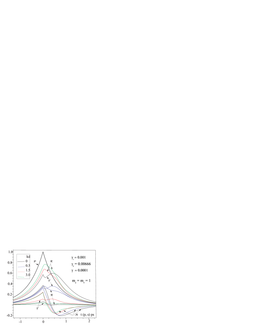
Figure 5: Same as in Fig.1 for four magnitudes of the parameter $kd$ in the case, when $\Delta\omega$ is close to $\gamma_{\,r},\gamma_{\,\ell\,}\gg\gamma_{\,r}\gg\gamma.$

The oscillation period in Fig.2 and 4 does not depend on the parameter $kd$, since, at chosen magnitudes of the parameters $\Delta\omega$ and $\gamma_{\,r}$ the beating frequency (36) is almost equal to $\omega_{1}-\omega_{2}$, and comparatively small changes of the functions $\varepsilon^{\prime}$ and $\varepsilon^{\prime\prime}$ does not affect practically on the beating frequency.

In Fig.5, where $\Delta\omega$ is near $\gamma_{\,r}$ ($6.65.10^{-3}eV$ and $6.66.10^{-3}eV$, respectively), the stimulating light pulse is 5 times shorter, than in Fig.3 and 4, and $\gamma_{\,\ell}\gg\gamma_{\,r}\gg\gamma$. In that case, the spatial dispersion affects strongly on the optical characteristics. In the interval $0\leq kd\leq 3$, the reflectance increases 8 times approximately, and the transmittance decreases 6 times. Such a sharp change is due to the dependence of $\bar{\gamma}_{\,r1}$ and $\bar{\gamma}_{\,r2}$ on $kd$. For example, at $kd=0$ $\bar{\gamma}_{\,r1}=-17303.9,\bar{\gamma}_{\,r2}=193066,6$, and at $kd=3$ $Re\,\bar{\gamma}_{\,r1}=1960.21,Re\,\bar{\gamma}_{\,r2}=442,718$. And at the same time, ${\cal R}$ and ${\cal T}~{}~{}\leq 1$, since they are the result of substraction of large magnitudes and therefore these differences are sensitive to changes of $kd$.

In bb14 , it was shown that, at $kd=0$, there are the singular points on the time axis, where ${\cal T}={\cal A}=0$ and ${\cal R}={\cal P}$, or ${\cal R}={\cal A}=0$ and ${\cal T}={\cal P}$ (total reflection or total transmission). It is seen from the figures that the singular points are preserved and in the case $kd\neq 0$, there is only a small shift of them. In Fig.5 the point of the total transmission appears at $kd=0$. At $kd=0.5$, this point disappears, and at $kd=1.5$ and $kd=3.0$ the point of the total reflection appears. If $kd=1.5$, then ${\cal R}={\cal P}$, ${\cal A}+{\cal T}=0~{}~{}({\cal A}<0)$. If $kd=3.0$, then as before ${\cal R}={\cal P}$, but ${\cal A}={\cal T}=0$. Thus, growing of the parameter $kd$ changes the type of a singular point.

Thus, the spatial dispersion of the electromagnetic waves, forming the light pulse, noticeably affect the optical characteristics of a quantum well. This influence is especially strong, when $\gamma_{\,r}\simeq\Delta\omega$.

Let us note in conclusion that the results obtained above are valid at equal refraction indices of barriers and quantum well. Otherwise, one is to take into account reflection of boundaries of a quantum well. However, this problem is outside the scopes of present article.

References

(1)
L. C. Andreani, F. Tassone, F. Bassani. Sol. State Commun. 77, 9, 641 (1991).
(2)
L. C. Andreani. In: Confined electrons and phonons. Eds E.
Burstein, C. Weisbuch, Plenum Press, N. Y. (1995), p. 57.
(3)
E. L. Ivchenko. Fiz. Tverd. Tela, 1991, 33, N 8, 2388
(Physics of the Solid State (St. Petersburg), 33,
2182 (1991)).
(4)
F. Tassone, F. Bassani, L. C. Andreani. Phys. Rev. B 45, 11,
6023 (1992).
(5)
T.Stroucken, A. Knorr, C. Anthony, P. Thomas, S. W. Koch, M. Koch,
S. T. Gundiff, J. Feldman, E. O. Gbel. Phys. Rev. Lett.
74, 9, 2391 (1996).
(6)
T.Stroucken, A. Knorr, P. Thomas, S. W. Koch. Phys. Rev. B 53, 4, 2026 (1996).
(7)
L. C. Andreani, G. Panzarini, A. V. Kavokin, M. R. Vladimirova.
Phys. Rev. B 57, 8, 4670 (1998).
(8)
M. Hbner, T. Kuhl, S. Haas, T.Stroucken, S. W. Koch, R.
Hey, K. Ploog. Sol. State Commun., 105, 2, 105 (1998).
(9)
L. I. Korovin, I. G. Lang, D. A. Contreras-Solorio, S. T. Pavlov.
Fiz. Tverd. Tela, 43, 2091 (2001) (Physics of the Solid
State (St. Petersburg), 43, 2182 (2001)); cond-mat/0104262.
(10)
I. G Lang, V. I. Belitsky, M. Cardona. Phys. Stat. Sol. (a) 164, 1, 307 (1997).
(11)
I. G Lang, V. I. Belitsky. Solid. State Commun. 107, 10, 577
(1998).
(12)
I. G Lang, V. I. Belitsky. Phys. Lett. A 245, 329 (1998).
(13)
I. G. Lang, L. I. Korovin, A. Contreras-Solorio, S. T. Pavlov.
Fiz. Tverd. Tela, 43, 1117 (2001) (Physics of the Solid
State (St. Petersburg), 43, 1159 (2001)); cond-mat/ 0004178.
(14)
D. A. Contreras-Solorio, S. T. Pavlov, L. I. Korovin, I. G. Lang.
Phys. Rev 62, 24, 16815 (2000); cond-mat/0002229.
(15)
I. G. Lang, L. I. Korovin, A. Contreras-Solorio, S. T. Pavlov.
Fiz. Tverd. Tela, 42, 2230 (2000) ( Physics of the Solid
State (St. Petersburg) , 42, N 12, 2300 (2000));
cond-mat/0006364.
(16)
L. I. Korovin, I. G. Lang, D. A. Contreras-Solorio, S. T. Pavlov.
Fiz. Tverd. Tela, 44, 1681 (2002) (Physics of the Solid
State (St. Petersburg), 44, 1759 (2002)); cond-mat/0203390.
(18)
I. G. Lang, L. I. Korovin, A. Contreras-Solorio, S. T. Pavlov,
Fiz. Tverd.Tela, 44, 2084 (2002) (Physics of the Solid State
(St. Petersburg), 44, 2181 (2002)); cond-mat/ 0001248.
(19)
I. G. Lang, L. I. Korovin, A. Contreras-Solorio, S. T. Pavlov.
Fiz. Tverd.Tela, 48, 1795 (2006) (Physics of the Solid State
(St. Petersburg), 48, 1693 (2006)); cond-mat/ 0403302.
(20)
L. I. Korovin, I. G. Lang, S. T. Pavlov.
Fiz. Tverd.Tela, 48, 2208 (2006) (Physics of the Solid State (St.
Petersburg), 48, 2337 (2006)); cond-mat/ 0001248.
(21)
L. I. Korovin, I. G. Lang, S. T. Pavlov.
Zh. Eksp. Teor. Fiz., 115, 187 (1999) (JETP, 88, 105 (1999)).