Pair production with neutrinos in an intense background magnetic field

Abstract

We present a detailed calculation of the electron-positron production rate using neutrinos in an intense background magnetic field. The computation is done for the process $\nu\to\nu e\bar{e}$ (where $\nu$ can be $\nu_{e}$, $\nu_{\mu}$, or $\nu_{\tau}$) within the framework of the Standard Model. Results are given for various combinations of Landau-levels over a range of possible incoming neutrino energies and magnetic field strengths.

I Introduction

Neutrino interactions are of great importance in astrophysics because of their capacity to serve as mediators for the transport and loss of energy. Their low mass and weak couplings make neutrinos ideal candidates for this role. Therefore, the rates of neutrino interactions are integral in the evolution of all stars, particularly the collapse and subsequent explosion of supernovae, where the overwhelming majority of gravitational energy lost is radiated away in the form of neutrinos.

Neutrinos have held a prominent place in models of stellar collapse ever since Gamow and Schoenberg suggested their role in 1941 Gamow and Schoenberg (1941). While supernova models have progressed a great deal in the last 65 years, the precise mechanism for explosion is still uncertain. A common feature, however, among all models is the sensitivity to neutrino transport. Neutrino processes once thought to be negligible now become relevant, and this has inspired many authors to calculate rates for neutrino interactions beyond that of the fundamental “Urca” processes

$$p\ e \to n\ \nu_{e}$$

$$n \to p\ e\ \bar{\nu}_{e}\,.$$

Recent examples include neutrino-electron scattering, neutrino-nucleus inelastic scattering, and electron-positron pair annihilation Bruenn and Haxton (1991); Mezzacappa and Bruenn (1993). Furthermore, the large magnetic field strengths associated with supernovae ($10^{12}$–$10^{17}$ G) are likely to cause significant changes in the behavior of neutrino transport.

While the the electromagnetic field does not couple to the Standard Model neutrino, it does affect neutrino physics by altering the behavior of any charged particles, real or virtual, with which the neutrino may interact. A number of authors have considered such effects on Urca-type processes Dorofeev et al. (1984); Baiko and Yakovlev (1999); Gvozdev and Ognev (1999); Arras and Lai (1999) and on neutrino absorption by nucleons (and its reversed processes) Duan and Qian (2005); Bhattacharya and Pal (2004a); Bhattacharya (2004). Furthermore, Bhattacharya and Pal have prepared a very nice review of other processes involving neutrinos that are affected by the presence of a magnetic field Bhattacharya and Pal (2004b).

The problem of interest in this work is the production of electron-positron pairs with neutrinos in an intense magnetic field

$$\nu\ \to\ \nu\ e\ \bar{e}\,.$$ (1)

Normally this process is kinematically forbidden, but the presence of the magnetic field changes the energy balance of the process, thereby permitting the interaction.

Stimulation of this process with high-intensity laser fields has been shown to have an unacceptably low rate of production Tinsley (2005), but such an interaction could have important consequences in astrophysical phenomena where large magnetic field strengths exist. The process would most likely serve to transfer energy in core-collapse supernovae Thompson and Duncan (1993). However, Gvozdev et al. have proposed that its role in magnetars could even help to explain observed gamma-ray bursts Gvozdev et al. (1998). The interest in this reaction has led to a previous treatment in the literature Kuznetsov and Mikheev (1997), but those authors present results for two special limiting cases: (1) when the generalized magnetic field strength $eB$ is greater than the square of the initial neutrino energy $E^{2}$, and (2) when the square of the initial neutrino energy $E^{2}$ is much greater than the generalized magnetic field strength $eB$. In both cases the incoming neutrino energy $E$ is much greater than the electron’s rest energy $m_{e}$. In this paper we present a more complete calculation of the production rate as mediated by the neutral and the charged-current processes (FIG. 1). We present the results of the calculation for varying Landau levels, neutrino energies, and magnetic field strengths. A comparison with the approximate method is also discussed.

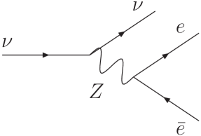
(a) Neutral current reaction

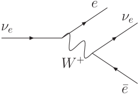
(b) Charged current reaction

Figure 1: Possible diagrams considered for the process $\nu\ \to\ \nu e\bar{e}$. Both diagrams contribute for electron-type neutrinos, but only the neutral current reaction (FIG. 1(a)) contributes for $\nu_{\mu}$ and $\nu_{\tau}$.

II Field operator solutions

As we have pointed out in section I, the standard model neutrino can only be affected by the electromagnetic field through its interactions with charged particles. This means that for the process $\nu\to\nu e\bar{e}$ the Dirac field solution for the final state electron and positron must change relative to their free-field solutions. The magnetic field will also change the form of the $W$-boson’s field solution which can mediate the process when electron neutrinos are considered. However, in our analysis we take the limit that the momentum transfer for this reaction is much less than the mass of the $W$-boson ($Q^{2}\ll m_{W}^{2}$) and ignore any effects the magnetic field may have on this charged boson. Thus, in this section we review the results of our derivation of the Dirac field operator solutions for the electron and positron. We closely follow the conventions used by Bhattacharya and Pal and refer the reader to their work Bhattacharya and Pal (2004a) for a detailed derivation. The reader who is familiar with these solutions may wish to begin with section III where we calculate the production rate.

We choose our magnetic field to lie along the positive $z$-axis

$$\vec{B}=B_{0}\hat{k}$$ (2)

which allows us some freedom in the choice of vector potential $A(x)$. We make the choice

$$A^{\mu}(x)=\left(0,-yB,0,0\right)$$ (3)

both for its simplicity and its agreement with the choice found in reference Bhattacharya and Pal (2004a). This choice in vector potential leads us to assume that all of the $y$ space-time coordinate dependence is within the spinors. The absence of any $y$ dependence in, for instance, the phase leads us to define a notation such that

$${y\!\!\!\!-}^{\mu}=\left(t,x,0,z\right)\,$$ (4)

and

$$\vec{V}_{{y\!\!\!\!-}}=\left(V_{x},0,V_{z}\right)\,,$$ (5)

where $\vec{V}$ is any 3-vector.

II.1 Electron field operator

Solving the Dirac equation for our choice of vector potential (Eq. 3) results in the following electron field operator

$$\psi_{e}(x)=\sum_{n=0}^{\infty}\sum_{s=\pm}\int\frac{\mathrm{d}^{2}\vec{p}_{{y\!\!\!\!-}}}{(2\pi)^{2}}\sqrt{\frac{E_{n}+m_{e}}{2E_{n}}}\left[u^{s}(\vec{p}_{{y\!\!\!\!-}},n,y)\,e^{-ip\cdot{y\!\!\!\!-}}\,\hat{a}^{s}_{e\,\vec{p}_{{y\!\!\!\!-}},n}+v^{s}(\vec{p}_{{y\!\!\!\!-}},n,y)\,e^{+ip\cdot{y\!\!\!\!-}}\,{\hat{b}^{s\,{\dagger}}_{e\,\vec{p}_{{y\!\!\!\!-}},n}}\right]\,,$$ (6)

where the creation and annihilation operators obey the following anti-commutation relations

$$\left\{\hat{a}^{s}_{e\,\vec{p}_{{y\!\!\!\!-}},n},\hat{a}^{s^{\prime}\,{\dagger}}_{e\,{\vec{p}}^{\prime}_{{y\!\!\!\!-}},n^{\prime}}\right\}=\left\{\hat{b}^{s}_{e\,\vec{p}_{{y\!\!\!\!-}},n},\hat{b}^{s^{\prime}\,{\dagger}}_{e\,\vec{p}^{\prime}_{{y\!\!\!\!-}},n^{\prime}}\right\}=(2\pi)^{2}\,\delta^{ss^{\prime}}\,\delta_{nn^{\prime}}\,\delta^{2}(\vec{p}_{{y\!\!\!\!-}}-\vec{p}_{{y\!\!\!\!-}}\,\!^{\prime})\,.$$ (7)

In Eq. 6 we sum over all possible spins $s$ and all Landau levels $n$ where $E_{n}$ is the energy of fermion occupying the $n^{\mathrm{th}}$ Landau level

$$E_{n}=\sqrt{p_{z}^{2}+m_{e}^{2}+2neB}\,,\qquad n\geq 0\,.$$ (8)

The Dirac bi-spinors are

$$u^{+}(\vec{p}_{{y\!\!\!\!-}},n,y)=\left(\begin{array}[]{c}I_{n-1}(\xi_{-})\\ 0\\ \frac{p_{z}}{E_{n}+m_{e}}I_{n-1}(\xi_{-})\\ -\frac{\sqrt{2neB}}{E_{n}+m_{e}}I_{n}(\xi_{-})\end{array}\right)\,,\qquad u^{-}(\vec{p}_{{y\!\!\!\!-}},n,y)=\left(\begin{array}[]{c}0\\ I_{n}(\xi_{-})\\ -\frac{\sqrt{2neB}}{E_{n}+m_{e}}I_{n-1}(\xi_{-})\\ -\frac{p_{z}}{E_{n}+m_{e}}I_{n}(\xi_{-})\end{array}\right)\,,$$ (9a)

and

$$v^{+}(\vec{p}_{{y\!\!\!\!-}},n,y)=\left(\begin{array}[]{c}\frac{p_{z}}{E_{n}+m_{e}}I_{n-1}(\xi_{+})\\ \frac{\sqrt{2neB}}{E_{n}+m_{e}}I_{n}(\xi_{+})\\ I_{n-1}(\xi_{+})\\ 0\end{array}\right)\,,\qquad v^{-}(\vec{p}_{{y\!\!\!\!-}},n,y)=\left(\begin{array}[]{c}\phantom{-}\frac{\sqrt{2neB}}{E_{n}+m_{e}}I_{n-1}(\xi_{+})\\ -\frac{p_{z}}{E_{n}+m_{e}}I_{n}(\xi_{+})\\ 0\\ I_{n}(\xi_{+})\end{array}\right)\,.$$ (9b)

The $I_{m}(\xi)$ are functions of the Hermite polynomials

$$I_{m}(\xi)=\left(\frac{\sqrt{eB}}{2^{m}\,m!\,\sqrt{\pi}}\right)^{1/2}e^{-\xi^{2}/2}\,H_{m}(\xi)$$ (10)

where the dimensionless parameter $\xi$ is defined by

$$\xi_{\pm}=\sqrt{eB}\,y\pm\frac{p_{x}}{\sqrt{eB}}\,.$$ (11)

Recall that the Hermite polynomials $H_{m}(\xi)$ are only defined for nonnegative values of $m$. Therefore, we must define $I_{-1}(\xi)=0$. This means that the electron in the lowest Landau energy level ($n=0$) cannot exist in spin-up state and the positron in the lowest Landau energy level cannot exist in the spin-down state.

The normalization in Eq. (10) has been chosen such that the functions $I_{m}(\xi)$ obey the following delta-function representation (Arfken and Weber, 1995, p. 86)

$$\delta(y-y^{\prime}) = \frac{\delta(\xi-\xi^{\prime})}{\left|\partial y/\partial{\xi}\right|}$$

$$= \sqrt{eB}\,\delta(\xi-\xi^{\prime})$$

$$= \sqrt{eB}\,\sum_{n=0}^{\infty}\frac{1}{2^{n}\,n!\,\sqrt{\pi}}\,e^{-\xi^{2}/2}\,H_{n}(\xi)\,e^{-\xi^{\prime 2}/2}\,H_{n}(\xi^{\prime})$$

$$\delta(y-y^{\prime}) = \sum_{n=0}^{\infty}I_{n}(\xi)I_{n}(\xi^{\prime})\,.$$ (12)

For convenience we choose to normalize our 1-particle states in a “box” with dimensions $L_{x}L_{y}L_{z}=V$ such that the states are defined as

$$|e\rangle=\left|\vec{p}_{1{y\!\!\!\!-}},n_{1},s_{1}\right\rangle=\frac{1}{\sqrt{L_{x}Lz}}\,\hat{a}^{s_{1}\,{\dagger}}_{e\,{\vec{p}}_{1{y\!\!\!\!-}},n_{1}}\,|0\rangle\,\phantom{,}$$ (13a)

$$|\bar{e}\rangle=\left|\vec{p}_{2{y\!\!\!\!-}},n_{2},s_{2}\right\rangle=\frac{1}{\sqrt{L_{x}Lz}}\,\hat{b}^{s_{2}\,{\dagger}}_{e\,{\vec{p}}_{2{y\!\!\!\!-}},n_{2}}\,|0\rangle\,,$$ (13b)

and the completeness relation for the states is

$$1=\sum_{n=0}^{\infty}\sum_{s=\pm}\int\frac{\mathrm{d}^{2}\vec{p}_{{y\!\!\!\!-}}}{(2\pi)^{2}}L_{x}L_{z}\left|\vec{p}_{{y\!\!\!\!-}},n,s\right\rangle\left\langle\vec{p}_{{y\!\!\!\!-}},n,s\right|\,.$$ (14)

II.2 Spin sums

In order to evaluate the production rate for our process, we must derive the completeness relations for summations over the spin of the fermions. For a detailed calculation of the rules see reference Bhattacharya (2004). The results of the calculation are as follows

$$\sum_{s=+,-}u^{s}(\vec{p}_{{y\!\!\!\!-}},n,y^{\prime})\bar{u}^{s}(\vec{p}_{{y\!\!\!\!-}},n,y) = \left(2(E_{n}+m_{e})\right)^{-1}\biggl{\{}\ \left[m_{e}(1-\sigma^{3})+\not\!{p}_{\parallel}+\not\!{q}_{\parallel}\gamma^{5}\right]I_{n}(\xi_{-}^{\prime})I_{n}(\xi_{-})$$ (15a)

$$\phantom{\left(2(E_{n}+m_{e})\right)^{-1}}+\left[m_{e}(1+\sigma^{3})+\not\!{p}_{\parallel}-\not\!{q}_{\parallel}\gamma^{5}\right]I_{n-1}(\xi_{-}^{\prime})I_{n-1}(\xi_{-})$$

$$\phantom{\left(2(E_{n}+m_{e})\right)^{-1}}+\sqrt{2neB}\left(\gamma^{1}+i\gamma^{2}\right)I_{n-1}(\xi_{-}^{\prime})I_{n}(\xi_{-})$$

$$\phantom{\left(2(E_{n}+m_{e})\right)^{-1}}+\sqrt{2neB}\left(\gamma^{1}-i\gamma^{2}\right)I_{n}(\xi_{-}^{\prime})I_{n-1}(\xi_{-})\biggr{\}}$$

and

$$\sum_{s=\pm}v^{s}(\vec{p}_{{y\!\!\!\!-}},n,y)\bar{v}^{s}(\vec{p}_{{y\!\!\!\!-}},n,y^{\prime}) = \left(2(E_{n}+m_{e})\right)^{-1}\biggl{\{}\ \left[-m_{e}(1-\sigma^{3})+\not\!{p}_{\parallel}+\not\!{q}_{\parallel}\gamma^{5}\right]I_{n}(\xi_{+})I_{n}(\xi_{+}^{\prime})$$ (15b)

$$\phantom{\left(2(E_{n}+m_{e})\right)^{-1}}+\left[-m_{e}(1+\sigma^{3})+\not\!{p}_{\parallel}-\not\!{q}_{\parallel}\gamma^{5}\right]I_{n-1}(\xi_{+})I_{n-1}(\xi_{+}^{\prime})$$

$$\phantom{\left(2(E_{n}+m_{e})\right)^{-1}}-\sqrt{2neB}\left(\gamma^{1}+i\gamma^{2}\right)I_{n-1}(\xi_{+})I_{n}(\xi_{+}^{\prime})$$

$$\phantom{\left(2(E_{n}+m_{e})\right)^{-1}}-\sqrt{2neB}\left(\gamma^{1}-i\gamma^{2}\right)I_{n}(\xi_{+})I_{n-1}(\xi_{+}^{\prime})\biggr{\}}\,,$$

where

$$p_{\parallel}^{\mu} = (E,0,0,p_{z})$$ (16)

$$q_{\parallel}^{\mu} = (p_{z},0,0,E)\,.$$ (17)

The above results have been derived using the standard “Bjorken and Drell” representation for the $\gamma$-matrices Bjorken and Drell (1964)

$$\gamma^{0}=\left(\begin{array}[]{cc}1&0\\ 0&-1\end{array}\right)\,,\qquad\gamma^{i}=\left(\begin{array}[]{cc}0&\sigma^{i}\\ -\sigma^{i}&0\end{array}\right)\,.$$ (18)

II.3 Neutrino field operator

Having no charge, the neutrino’s field operator solution $\psi_{\nu}(x)$ is not modified due to the magnetic field. We present it here for easy reference

$$\psi_{\nu}(x)=\sum_{s=\pm}\int\frac{\mathrm{d}^{3}\vec{p}}{(2\pi)^{3}}\left[u^{s}(p)\,e^{-ip\cdot x}\,\hat{a}^{s}_{\nu}+v^{s}(p)\,e^{+ip\cdot x}\,{\hat{b}^{s\,{\dagger}}_{\nu}}\right]\,,$$ (19)

where the creation and annihilation operators obey the conventional anticommutation relations

$$\left\{\hat{a}^{s}_{\nu},\hat{a}^{s^{\prime}\,{\dagger}}_{\nu}\right\}=\left\{\hat{b}^{s}_{\nu},\hat{b}^{s^{\prime}\,{\dagger}}_{\nu}\right\}=(2\pi)^{3}\,\delta^{ss^{\prime}}\,\delta^{3}(\vec{p}-\vec{p}\,^{\prime})\,.$$ (20)

The neutrino bi-spinors follow the standard spin sum rules

$$\sum_{s=\pm}u^{s}(p)\bar{u}^{s}(p)=\sum_{s=\pm}v^{s}(p)\bar{v}^{s}(p)=\not\!{p}\,,$$ (21)

where we take the Standard Model neutrino mass to be zero.

With “box” normalization the 1-particle states for the neutrino are

$$|\nu\rangle=\left|\vec{p},s\right\rangle=\frac{1}{\sqrt{V}}\,\hat{a}^{s\,{\dagger}}_{\nu\,{\vec{p}}}\,|0\rangle\,,$$ (22)

satisfying the completeness relation

$$1=\sum_{s=\pm}\int\frac{\mathrm{d}^{3}\vec{p}}{(2\pi)^{3}}V\left|\vec{p},s\right\rangle\left\langle\vec{p},s\right|\,.$$ (23)

III The production rate

The quantity of interest for the process $\nu\to\nu e\bar{e}$ in a background magnetic field is the rate at which the electron-positron pairs are produced $\Gamma$. The production rate is defined as the probability per unit time for creation of pairs

$$\Gamma=\lim_{T\to\infty}\frac{\mathcal{P}}{T}\,.$$ (24)

where $T$ is the timescale on which the process is normalized. We begin by finding the probability $\mathcal{P}$ of our reaction

$$\mathcal{P}=\sum_{n_{1},n_{2}=0}^{\infty}\int\frac{\mathrm{d}^{3}\vec{p}^{\prime}}{(2\pi)^{3}}\,V\,\int\frac{\mathrm{d}^{2}\vec{p}_{1{y\!\!\!\!-}}}{(2\pi)^{2}}\,L_{x}L_{z}\,\int\frac{\mathrm{d}^{2}\vec{p}_{2{y\!\!\!\!-}}}{(2\pi)^{2}}\,L_{x}L_{z}\,\sum_{s,s^{\prime},s_{1},s_{2}}\left|\left\langle\vec{p}^{\prime},s^{\prime};\vec{p}_{1{y\!\!\!\!-}},n_{1},s_{1};\vec{p}_{2{y\!\!\!\!-}},n_{2},s_{2}\left|\hat{S}\right|\vec{p},s\right\rangle\right|^{2}\,.$$ (25)

In Eq. 25 quantities with the index $1$ correspond to the electron, those with index $2$ to the positron, the primed quantities to the final neutrino, and the unprimed quantities correspond to the initial neutrino.

III.1 The scattering matrix

The scattering matrix

$$S=\left\langle\vec{p}^{\prime},s^{\prime};\vec{p}_{1{y\!\!\!\!-}},n_{1},s_{1};\vec{p}_{2{y\!\!\!\!-}},n_{2},s_{2}\left|\hat{S}\right|\vec{p},s\right\rangle$$ (26)

naturally depends on the flavor of the neutrino. While the process involving the electron neutrino can advance through either the charged ($W$) or neutral ($Z$) current, the muon (or tau) neutrino can only proceed through the latter. For this reason we will break the scattering matrix into a neutral component

$$S_{Z}=\left\langle\vec{p}^{\prime},s^{\prime};\vec{p}_{1{y\!\!\!\!-}},n_{1},s_{1};\vec{p}_{2{y\!\!\!\!-}},n_{2},s_{2}\left|\hat{S}_{Z}\right|\vec{p},s\right\rangle$$ (27a)

and a charged component

$$S_{W}=\left\langle\vec{p}^{\prime},s^{\prime};\vec{p}_{1{y\!\!\!\!-}},n_{1},s_{1};\vec{p}_{2{y\!\!\!\!-}},n_{2},s_{2}\left|\hat{S}_{W}\right|\vec{p},s\right\rangle\,,$$ (27b)

where the scattering operators are defined by the Standard Model Lagrangian as

$$\hat{S}_{Z}=\frac{e^{2}}{2^{3}\,\cos^{2}\theta_{W}\,\sin^{2}\theta_{W}}\int\mathrm{d}^{4}x\,\overline{\psi}_{e}(x)\gamma^{\mu}\left(g_{V}^{e}-g_{A}^{e}\gamma^{5}\right)\psi_{e}(x)Z_{\mu}(x)\int\mathrm{d}^{4}x^{\prime}\,\overline{\psi}_{\nu_{l}}(x^{\prime})\gamma^{\sigma}\left(1-\gamma^{5}\right)\psi_{\nu_{l}}(x^{\prime})Z_{\sigma}(x^{\prime})$$ (28a)

$$\hat{S}_{W}=\frac{e^{2}}{2^{3}\,\sin^{2}\theta_{W}}\int\mathrm{d}^{4}x\,\overline{\psi}_{e}(x)\gamma^{\mu}\left(1-\gamma^{5}\right)\psi_{\nu_{e}}(x)W^{-}_{\mu}(x)\int\mathrm{d}^{4}x^{\prime}\,\overline{\psi}_{\nu_{e}}(x^{\prime})\gamma^{\sigma}\left(1-\gamma^{5}\right)\psi_{e}(x^{\prime})W^{+}_{\sigma}(x^{\prime})\,,$$ (28b)

and $\theta_{W}$ is the weak-mixing angle, $\nu_{l}$ indicates a neutrino of any flavor, $\nu_{e}$ refers to a electron neutrino, and the vector and axial vector couplings for the electron are

$$g_{V}^{e} = -\frac{1}{2}+2\sin^{2}\theta_{W}$$ (29a)

$$g_{A}^{e} = -\frac{1}{2}\,.$$ (29b)

In our analysis we will be using incoming neutrino energies that are well below the rest energies of the $Z$ and $W$ bosons. Therefore, we can safely make the 4-fermion effective coupling approximation to the $Z$ and $W$ propagators

$$\left\langle 0\left|T\left(Z_{\mu}(x)Z_{\sigma}(x^{\prime})\right)\right|0\right\rangle \to \delta^{4}(x-x^{\prime})\,\frac{g_{\mu\sigma}}{m_{Z}^{2}}$$ (30a)

$$\left\langle 0\left|T\left(W^{-}_{\mu}(x)W^{+}_{\sigma}(x^{\prime})\right)\right|0\right\rangle \to \delta^{4}(x-x^{\prime})\,\frac{g_{\mu\sigma}}{m_{W}^{2}}\,.$$ (30b)

After making this approximation our expressions for the scattering operators simplify to

$$\hat{S}_{Z} = \frac{G_{F}}{\sqrt{2}}\int\mathrm{d}^{4}x\,\overline{\psi}_{e}(x)\gamma^{\mu}\left(g_{V}^{e}-g_{A}^{e}\gamma^{5}\right)\psi_{e}(x)\,\overline{\psi}_{\nu_{l}}(x)\gamma_{\mu}\left(1-\gamma^{5}\right)\psi_{\nu_{l}}(x)\qquad$$ (31a)

$$\hat{S}_{W} = \frac{G_{F}}{\sqrt{2}}\int\mathrm{d}^{4}x\,\overline{\psi}_{e}(x)\gamma^{\mu}\left(1-\gamma^{5}\right)\psi_{\nu_{e}}(x)\,\overline{\psi}_{\nu_{e}}(x)\gamma_{\mu}\left(1-\gamma^{5}\right)\psi_{e}(x)\,,$$ (31b)

where $G_{F}/\sqrt{2}=e^{2}/(8\,\sin^{2}\theta_{W}\,m_{W}^{2})$, and we have made use of the fact that $\cos^{2}\theta_{W}=m_{W}^{2}/m_{Z}^{2}$.

After substituting of the scattering operators (Eqs. (31)) into the expressions for the components of the scattering matrix (Eqs. (27)), we can use our results from sections II.1 and II.3 to write the components in the form of

$$S_{Z/W}=\frac{i(2\pi)^{3}\,\delta^{3}\left(p_{{y\!\!\!\!-}}-p_{{y\!\!\!\!-}}^{\prime}-p_{{y\!\!\!\!-},1}-p_{{y\!\!\!\!-},2}\right)}{L_{x}\,L_{z}\,V}\,\mathcal{M}_{Z/W}\,,$$ (32)

where

$$\mathcal{M}_{Z} = \frac{-iG_{F}}{2^{2}\sqrt{2}}\,\sqrt{\frac{(E_{n_{1}}+m_{e})(E_{n_{2}}+m_{e})}{EE^{\prime}E_{n_{1}}E_{n_{2}}}}\,\bar{u}^{s^{\prime}}(p^{\prime})\gamma_{\mu}\left(1-\gamma^{5}\right)u^{s}(p)$$ (33a)

$$\times\int\mathrm{d}y\,e^{i(p_{y}-p^{\prime}_{y})y}\,\bar{u}^{s_{1}}\left(\vec{p}_{1{y\!\!\!\!-}},n_{1},y\right)\gamma^{\mu}\left(g_{V}^{e}-g_{A}^{e}\gamma^{5}\right)v^{s_{2}}\left(\vec{p}_{2{y\!\!\!\!-}},n_{2},y\right)\qquad$$

$$\mathcal{M}_{W} = \frac{iG_{F}}{2^{2}\sqrt{2}}\,\sqrt{\frac{(E_{n_{1}}+m_{e})(E_{n_{2}}+m_{e})}{EE^{\prime}E_{n_{1}}E_{n_{2}}}}\,\bar{u}^{s^{\prime}}(p^{\prime})\gamma_{\mu}\left(1-\gamma^{5}\right)v^{s_{2}}\left(\vec{p}_{2{y\!\!\!\!-}},n_{2},y\right)$$ (33b)

$$\times\int\mathrm{d}y\,e^{i(p_{y}-p^{\prime}_{y})y}\,\bar{u}^{s_{1}}\left(\vec{p}_{1{y\!\!\!\!-}},n_{1},y\right)\gamma^{\mu}\left(1-\gamma^{5}\right)u^{s}(p)\,.$$

The reversal of sign on Eq. (33b) relative to Eq. (33a) is from the anticommutation of the field operators. The scattering amplitude for the charged component $\mathcal{M}_{W}$ can be transformed into the form of the neutral component $\mathcal{M}_{Z}$ by making use of a Fierz rearrangement formula

$$\bar{u}_{1}\gamma_{\mu}\left(1-\gamma^{5}\right)u_{2}\,\bar{u}_{3}\gamma^{\mu}\left(1-\gamma^{5}\right)u_{4}=-\bar{u}_{1}\gamma_{\mu}\left(1-\gamma^{5}\right)u_{4}\,\bar{u}_{3}\gamma^{\mu}\left(1-\gamma^{5}\right)u_{2}\,,$$ (34)

such that

$$\mathcal{M}_{W} = \frac{-iG_{F}}{2^{2}\sqrt{2}}\,\sqrt{\frac{(E_{n_{1}}+m_{e})(E_{n_{2}}+m_{e})}{EE^{\prime}E_{n_{1}}E_{n_{2}}}}\,\bar{u}^{s^{\prime}}(p^{\prime})\gamma_{\mu}\left(1-\gamma^{5}\right)u^{s}(p)$$ (35)

$$\times\int\mathrm{d}y\,e^{i(p_{y}-p^{\prime}_{y})y}\,\bar{u}^{s_{1}}\left(\vec{p}_{1{y\!\!\!\!-}},n_{1},y\right)\gamma^{\mu}\left(1-\gamma^{5}\right)v^{s_{2}}\left(\vec{p}_{2{y\!\!\!\!-}},n_{2},y\right)\,.\qquad$$

With the rearrangement of $\mathcal{M}_{W}$ in Eq. (35), we can now express the scattering amplitude in terms of the type of incoming neutrino. The muon neutrino can only proceed through exchange of a $Z$-boson, so its scattering amplitude is just that of $\mathcal{M}_{Z}$

$$\mathcal{M}_{\nu_{\mu}} = \mathcal{M}_{Z}$$

$$\mathcal{M}_{\nu_{\mu}} = \frac{iG_{F}}{2^{3}\sqrt{2}}\,\sqrt{\frac{(E_{n_{1}}+m_{e})(E_{n_{2}}+m_{e})}{EE^{\prime}E_{n_{1}}E_{n_{2}}}}\,\bar{u}^{s^{\prime}}(p^{\prime})\gamma_{\mu}\left(1-\gamma^{5}\right)u^{s}(p)$$ (36)

$$\times\int\mathrm{d}y\,e^{i(p_{y}-p^{\prime}_{y})y}\,\bar{u}^{s_{1}}\left(\vec{p}_{1{y\!\!\!\!-}},n_{1},y\right)\gamma^{\mu}\left(G_{V}^{-}-\gamma^{5}\right)v^{s_{2}}\left(\vec{p}_{2{y\!\!\!\!-}},n_{2},y\right)\,.\qquad$$

The scattering matrix for a tau neutrino, and the subsequent decay rate, is exactly the same as the muon neutrino. We will keep the notation as $\nu_{\mu}$ for simplicity.

The electron neutrino has both a $Z$-boson exchange component and an $W$-boson exchange component. Therefore we must add the amplitudes to find its scattering amplitude

$$\mathcal{M}_{\nu_{e}} = \mathcal{M}_{Z}+\mathcal{M}_{W}$$

$$\mathcal{M}_{\nu_{e}} = \frac{-iG_{F}}{2^{3}\sqrt{2}}\,\sqrt{\frac{(E_{n_{1}}+m_{e})(E_{n_{2}}+m_{e})}{EE^{\prime}E_{n_{1}}E_{n_{2}}}}\,\bar{u}^{s^{\prime}}(p^{\prime})\gamma_{\mu}\left(1-\gamma^{5}\right)u^{s}(p)$$ (37)

$$\times\int\mathrm{d}y\,e^{i(p_{y}-p^{\prime}_{y})y}\,\bar{u}^{s_{1}}\left(\vec{p}_{1{y\!\!\!\!-}},n_{1},y\right)\gamma^{\mu}\left(G_{V}^{+}-\gamma^{5}\right)v^{s_{2}}\left(\vec{p}_{2{y\!\!\!\!-}},n_{2},y\right)\,.$$

Note that the scattering amplitudes for electron (Eq. III.1) and non-electron neutrinos (Eq. III.1) depend on a generalized vector coupling $G_{V}$ defined by

$$G_{V}^{\pm}=1\pm 4\sin^{2}\theta_{W}\,.$$ (38)

We see that the scattering amplitudes for an incoming electron neutrino versus an incoming muon neutrino differ only in the value of the generalized vector coupling and an overall sign. And the overall sign will be rendered meaningless once the amplitude is squared. Therefore, we choose to make no distinction between the two processes, other than keeping the generalized vector coupling as $G_{V}^{\pm}$, until we discuss the results in section IV.

III.2 The form of the production rate

Having determined the scattering matrix $S$ and scattering amplitude $\mathcal{M}$ in section III.1, we can now make series of substitutions of those results to find the expression for the production rate $\Gamma$. We begin by substituting the form of the scattering matrix (Eq. (32)) into the expression for the production rate (Eq. (24)

$$\Gamma = \lim_{T\to\infty}\frac{\mathcal{P}}{T}$$

$$= \lim_{T,V\to\infty}T^{-1}\,\sum_{n_{1},n_{2}=0}^{\infty}\int\frac{\mathrm{d}^{3}\vec{p}^{\prime}}{(2\pi)^{3}}\,V\,\int\frac{\mathrm{d}^{2}\vec{p}_{1{y\!\!\!\!-}}}{(2\pi)^{2}}\,L_{x}L_{z}\,\int\frac{\mathrm{d}^{2}\vec{p}_{2{y\!\!\!\!-}}}{(2\pi)^{2}}\,L_{x}L_{z}\sum_{s,s^{\prime},s_{1},s_{2}}\left|\left\langle\vec{p}^{\prime},s^{\prime};\vec{p}_{1{y\!\!\!\!-}},n_{1},s_{1};\vec{p}_{2{y\!\!\!\!-}},n_{2},s_{2}\left|\hat{S}\right|\vec{p},s\right\rangle\right|^{2}$$

$$= \lim_{T,V\to\infty}T^{-1}\,\sum_{n_{1},n_{2}=0}^{\infty}\int\frac{\mathrm{d}^{3}\vec{p}^{\prime}}{(2\pi)^{3}}\,V\,\int\frac{\mathrm{d}^{2}\vec{p}_{1{y\!\!\!\!-}}}{(2\pi)^{2}}\,L_{x}L_{z}\,\int\frac{\mathrm{d}^{2}\vec{p}_{2{y\!\!\!\!-}}}{(2\pi)^{2}}\,L_{x}L_{z}\sum_{s,s^{\prime},s_{1},s_{2}}\left|\frac{i(2\pi)^{3}\,\delta^{3}\left(p_{{y\!\!\!\!-}}-p_{{y\!\!\!\!-}}^{\prime}-p_{{y\!\!\!\!-},1}-p_{{y\!\!\!\!-},2}\right)}{L_{x}\,L_{z}\,V}\,\mathcal{M}\right|^{2}$$

$$\Gamma = \lim_{T,V\to\infty}(2\pi TV)^{-1}\,\sum_{n_{1},n_{2}=0}^{\infty}\int\mathrm{d}^{3}\vec{p}^{\prime}\,\int\mathrm{d}^{2}\vec{p}_{1{y\!\!\!\!-}}\,\int\mathrm{d}^{2}\vec{p}_{2{y\!\!\!\!-}}\left(\delta^{3}(p_{{y\!\!\!\!-}}-p_{{y\!\!\!\!-}}^{\prime}-p_{{y\!\!\!\!-},1}-p_{{y\!\!\!\!-},2})\right)^{2}\overline{\left|\mathcal{M}\right|^{2}}\,,\qquad$$ (39)

where $\overline{\left|\mathcal{M}\right|^{2}}$ is the square of the scattering amplitude after summing over spins

$$\overline{\left|\mathcal{M}\right|^{2}}=\sum_{s,s^{\prime},s_{1},s_{2}}\left|\mathcal{M}\right|^{2}\,.$$ (40)

We can simplify the square of the 3-dimensional delta function by expressing one of the 3-dimensional delta functions as a series of integrals over space-time coordinates

$$\left(\delta^{3}(p_{{y\!\!\!\!-}}-p_{{y\!\!\!\!-}}^{\prime}-p_{{y\!\!\!\!-},1}-p_{{y\!\!\!\!-},2})\right)^{2}=\delta^{3}(p_{{y\!\!\!\!-}}-p_{{y\!\!\!\!-}}^{\prime}-p_{{y\!\!\!\!-},1}-p_{{y\!\!\!\!-},2})\,\int\frac{\mathrm{d}^{3}{y\!\!\!\!-}}{(2\pi)^{3}}\,e^{i(p-p^{\prime}-p_{1}-p_{2})\cdot\,{y\!\!\!\!-}}\,.$$ (41)

By using the remaining set of delta functions to reduce the exponential to unity, we can write the integrand in terms of the dimensions of our normalization “box”

$$\left(\delta^{3}(p_{{y\!\!\!\!-}}-p_{{y\!\!\!\!-}}^{\prime}-p_{{y\!\!\!\!-},1}-p_{{y\!\!\!\!-},2})\right)^{2} = \delta^{3}(p_{{y\!\!\!\!-}}-p_{{y\!\!\!\!-}}^{\prime}-p_{{y\!\!\!\!-},1}-p_{{y\!\!\!\!-},2})\,\int\frac{\mathrm{d}^{3}{y\!\!\!\!-}}{(2\pi)^{3}}$$

$$\left(\delta^{3}(p_{{y\!\!\!\!-}}-p_{{y\!\!\!\!-}}^{\prime}-p_{{y\!\!\!\!-},1}-p_{{y\!\!\!\!-},2})\right)^{2} = \delta^{3}(p_{{y\!\!\!\!-}}-p_{{y\!\!\!\!-}}^{\prime}-p_{{y\!\!\!\!-},1}-p_{{y\!\!\!\!-},2})\,\frac{TL_{x}L_{z}}{(2\pi)^{3}}\,.$$ (42)

With the above result for the square of the delta function, the production rate in Eq. (III.2) simplifies to

$$\Gamma=\lim_{L_{y}\to\infty}\sum_{n_{1},n_{2}=0}^{\infty}\int\mathrm{d}^{3}\vec{p}^{\prime}\,\int\mathrm{d}^{2}\vec{p}_{1{y\!\!\!\!-}}\,\int\mathrm{d}^{2}\vec{p}_{2{y\!\!\!\!-}}\,\delta^{3}(p_{{y\!\!\!\!-}}-p_{{y\!\!\!\!-}}^{\prime}-p_{{y\!\!\!\!-},1}-p_{{y\!\!\!\!-},2})\frac{\overline{\left|\mathcal{M}\right|^{2}}}{(2\pi)^{4}L_{y}}\,.$$ (43)

The square of the scattering amplitude goes as the product of two traces

$$\overline{\left|\mathcal{M}\right|^{2}} = \sum_{s,s^{\prime},s_{1},s_{2}}\left|\mathcal{M}\right|^{2}$$

$$= \frac{G_{F}^{2}}{2^{7}}\,\frac{(E_{n_{1}}+m_{e})(E_{n_{2}}+m_{e})}{EE^{\prime}E_{n_{1}}E_{n_{2}}}$$

$$\times\sum_{s,s^{\prime}}\bar{u}^{s}(p)\gamma_{\sigma}\left(1-\gamma^{5}\right)u^{s^{\prime}}(p^{\prime})\bar{u}^{s^{\prime}}(p^{\prime})\gamma_{\mu}\left(1-\gamma^{5}\right)u^{s}(p)\int\mathrm{d}y\,e^{i(p_{y}-p^{\prime}_{y})y}\,\int\mathrm{d}y^{\prime}\,e^{-i(p_{y}-p^{\prime}_{y})y^{\prime}}$$

$$\times\sum_{s_{1},s_{2}}\bar{v}^{s_{2}}\left(\vec{p}_{2{y\!\!\!\!-}},n_{2},y^{\prime}\right)\gamma^{\sigma}\left(G_{V}^{\pm}-\gamma^{5}\right)u^{s_{1}}\left(\vec{p}_{1{y\!\!\!\!-}},n_{1},y^{\prime}\right)\bar{u}^{s_{1}}\left(\vec{p}_{1{y\!\!\!\!-}},n_{1},y\right)\gamma^{\mu}\left(G_{V}^{\pm}-\gamma^{5}\right)v^{s_{2}}\left(\vec{p}_{2{y\!\!\!\!-}},n_{2},y\right)$$

$$\overline{\left|\mathcal{M}\right|^{2}} = \frac{G_{F}^{2}}{2^{9}}\,\left(EE^{\prime}E_{n_{1}}E_{n_{2}}\right)^{-1}\,\int\mathrm{d}y\,e^{i(p_{y}-p^{\prime}_{y})y}\,\int\mathrm{d}y^{\prime}\,e^{-i(p_{y}-p^{\prime}_{y})y^{\prime}}\mathrm{Tr}\left\{\gamma_{\sigma}\left(1-\gamma^{5}\right)\not\!{p}^{\prime}\gamma_{\mu}\left(1-\gamma^{5}\right)\not\!{p}\right\}$$

$$\times\mathrm{Tr}\biggl{\{}\gamma^{\sigma}\left(G_{V}^{\pm}-\gamma^{5}\right)\Bigl{[}\left(m_{e}(1-\sigma^{3})+\not\!{p}_{1\parallel}+\not\!{q}_{1\parallel}\gamma^{5}\right)I_{n_{1}}(\xi_{-,1}^{\prime})I_{n_{1}}(\xi_{-,1})$$

$$\phantom{\times\mathrm{Tr}\ \gamma^{\sigma}\left(G_{V}^{\pm}-\gamma^{5}\right)}+\sqrt{2n_{1}eB}\left(\gamma^{1}+i\gamma^{2}\right)I_{n_{1}-1}(\xi_{-,1}^{\prime})I_{n_{1}}(\xi_{-,1})$$

$$\phantom{\times\mathrm{Tr}\ \gamma^{\sigma}\left(G_{V}^{\pm}-\gamma^{5}\right)}+\sqrt{2n_{1}eB}\left(\gamma^{1}-i\gamma^{2}\right)I_{n_{1}}(\xi_{-,1}^{\prime})I_{n_{1}-1}(\xi_{-,1})$$

$$\phantom{\times\mathrm{Tr}\ \gamma^{\sigma}\left(G_{V}^{\pm}-\gamma^{5}\right)}+\left(m_{e}(1+\sigma^{3})+\not\!{p}_{1\parallel}-\not\!{q}_{1\parallel}\gamma^{5}\right)I_{n_{1}-1}(\xi_{-,1}^{\prime})I_{n_{1}-1}(\xi_{-,1})\Bigr{]}$$

$$\phantom{\mathrm{Tr}\biggl{\{}}\times\gamma^{\mu}\left(G_{V}^{\pm}-\gamma^{5}\right)\Bigl{[}\left(-m_{e}(1-\sigma^{3})+\not\!{p}_{2\parallel}+\not\!{q}_{2\parallel}\gamma^{5}\right)I_{n_{2}}(\xi_{+,2}^{\prime})I_{n_{2}}(\xi_{+,2})$$

$$\phantom{\times\mathrm{Tr}\ \gamma^{\sigma}\left(G_{V}^{\pm}-\gamma^{5}\right)}-\sqrt{2n_{2}eB}\left(\gamma^{1}+i\gamma^{2}\right)I_{n_{2}-1}(\xi_{+,2}^{\prime})I_{n_{2}}(\xi_{+,2})$$

$$\phantom{\times\mathrm{Tr}\ \gamma^{\sigma}\left(G_{V}^{\pm}-\gamma^{5}\right)}-\sqrt{2n_{2}eB}\left(\gamma^{1}-i\gamma^{2}\right)I_{n_{2}}(\xi_{+,2}^{\prime})I_{n_{2}-1}(\xi_{+,2})$$

$$\phantom{\times\mathrm{Tr}\ \gamma^{\sigma}\left(G_{V}^{\pm}-\gamma^{5}\right)}+\left(-m_{e}(1+\sigma^{3})+\not\!{p}_{2\parallel}-\not\!{q}_{2\parallel}\gamma^{5}\right)I_{n_{2}-1}(\xi_{+,2}^{\prime})I_{n_{2}-1}(\xi_{+,2})\Bigr{]}\biggr{\}},$$

where we have used our result for the summations over spin from Eqs. (15) and (21).

The space-time dependence of Eq. (III.2) can be factored into terms like

$$I_{n,m}=\int\mathrm{d}y\,e^{i(p_{y}-p^{\prime}_{y})y}\,I_{n}(\xi_{-,1})\,I_{m}(\xi_{+,2})$$ (45)

and

$$I^{\ast}_{n,m}=\int\mathrm{d}y^{\prime}\,e^{-i(p_{y}-p^{\prime}_{y})y^{\prime}}\,I_{n}(\xi^{\prime}_{-,1})\,I_{m}(\xi_{+,2}^{\prime})\,,$$ (46)

where the $I_{n,m}$ are functions of the momenta in the problem.

We have included a detailed calculation for the general form of $I_{n,m}$ in appendix A, but we only present the result here

$$I_{n,m}=\left\{\begin{array}[]{l l}\sqrt{\frac{n!}{m!}}\,e^{-\eta^{2}/2}\,e^{i\phi_{0}}\left(\eta_{x}+i\eta_{y}\right)^{m-n}L_{n}^{m-n}\left(\eta^{2}\right)\,,&m\geq n\geq 0\\ \sqrt{\frac{m!}{n!}}\,e^{-\eta^{2}/2}\,e^{i\phi_{0}}\left(-\eta_{x}+i\eta_{y}\right)^{n-m}L_{m}^{n-m}\left(\eta^{2}\right)\,,&n\geq m\geq 0\end{array}\right\}\,$$ (47)

where

$$\eta_{x} = \frac{p_{1x}+p_{2x}}{\sqrt{2eB}}$$ (48)

$$\eta_{y} = \frac{p_{y}-p_{y}^{\prime}}{\sqrt{2eB}}$$ (49)

$$\phi_{0} = \frac{(p_{y}-p_{y}^{\prime})(p_{1}-p_{2})}{2eB}$$ (50)

$$\eta^{2} = \eta_{x}^{2}+\eta_{y}^{2}\,,$$ (51)

and $L_{n}^{m-n}(\eta^{2})$ are the associated Laguerre polynomials.

The full results of the traces and their subsequent contraction are nontrivial but have been included in appendix B. It is important to note, however, that the only dependence on the $x$-components of the electron and positron momentum is that which appears in Eq. (47) for $I_{n,m}$. Furthermore, we notice that all terms in the averaged square of the scattering amplitude have factors that go as a product of $I_{n,m}$ and $I^{\ast}_{n^{\prime},m^{\prime}}$. Therefore, the coefficient $e^{i\,\phi_{0}}$ in Eq. (47) will vanish when this product is taken. The only remaining $x$-dependence of these two momenta appear as their sum in the parameter $\eta_{x}=(p_{1x}+p_{2x})/\sqrt{2eB}$. This helps to simplify the phase-space integral for our production rate (Eq. (43)) which is proportional to

$$\Gamma\propto\lim_{L_{y}\to\infty}\frac{1}{L_{y}}\int\mathrm{d}p_{1\,x}\,\int\mathrm{d}p_{2\,x}\,.$$ (52)

If we make a change of variable from the $x$-component of the positron momentum $p_{2\,x}$ to the parameter $\eta_{x}$, the relationship in Eq. (52) is rewritten as

$$\Gamma\propto\lim_{L_{y}\to\infty}\frac{\sqrt{2eB}}{L_{y}}\int\mathrm{d}p_{1\,x}\,\int\mathrm{d}\eta_{x}\,.$$ (53)

Because there is no longer any explicit dependence on the $x$-component of the electron’s momentum $p_{1,x}$ in the averaged square of our scattering amplitude, we can simply evaluate the integral

$$\int\mathrm{d}p_{1,x}\,.$$

To evaluate this integral we must determine its limits. As discussed previously, we have elected to use “box” normalization on our states. This means that our particle is confined to a large box with dimensions $L_{x}$, $L_{y}$, and $L_{z}$. The careful reader will note that we have already taken the limit that these dimensions go

to infinity in some places, particularly in Eq. (67), but it is imperative that we be cautious here, as we could naively evaluate the integral over $p_{1,x}$ to be infinite.

Physically, the charged particles in our final state act as harmonic oscillators circling about the magnetic field lines. While they are free to slide about the lines along the $z$-axis, the particles are confined to circular orbits in the $x$ and $y$-directions no larger than the dimensions of the box. For a charged particle undergoing circular motion in a constant magnetic field, the $x$-component of momentum is related to the $y$-position vector by

$$p_{x}=-eQBy\,$$ (54)

where $Q$ is the charge of the particle in units of the proton charge $e=|e|$. Therefore, the limits on $p_{1,x}$ are proportional to the limits on the size of our box in the $y$-direction. The integral over the electron’s momentum in the $x$-direction is

$$\int_{-eBL_{y}/2}^{eBL_{y}/2}\mathrm{d}p_{1,x}=eBL_{y}\,,$$ (55)

and the result helps to cancel the factor of $L_{y}$ that already appears in the form of the production rate. We can now safely take the limit that our box has infinite size, and the production rate now has the form

$$\Gamma=\sum_{n_{1},n_{2}=0}^{\infty}\int\mathrm{d}^{3}\vec{p}^{\prime}\,\int\mathrm{d}\vec{p}_{1z}\,\int\mathrm{d}\vec{p}_{2z}\,\int\mathrm{d}\eta_{x}\,\sqrt{2eB}\,\delta^{3}(p_{{y\!\!\!\!-}}-p_{{y\!\!\!\!-}}^{\prime}-p_{{y\!\!\!\!-},1}-p_{{y\!\!\!\!-},2})\,\frac{eB\,\overline{\left|\mathcal{M}\right|^{2}}}{(2\pi)^{4}}\,.$$ (56)

IV Results

In our expression for the total production rate (Eq. (56)), one will notice is that there is a sum over all possible values of the Landau levels. As a consequence of energy conservation, upper limits do exist for the summation over the electron’s Landau level $n_{1}$

$$E = E^{\prime}+E_{n_{1}}+E_{n_{2}}$$

$$E \geq E_{n_{1}}+m_{e}$$

$$E-m_{e} \geq \sqrt{m_{e}^{2}+2n_{1}eB}$$

$$n_{1} \leq \frac{E(E-2m_{e})}{2eB}\,,$$ (57)

and a similar one for the positron’s Landau level

$$E = E^{\prime}+E_{n_{1}}+E_{n_{2}}$$

$$E \geq \sqrt{m_{e}^{2}+2n_{1}eB}+E_{n_{2}}$$

$$E-\sqrt{m_{e}^{2}+2n_{1}eB} \geq \sqrt{m_{e}^{2}+2n_{2}eB}$$

$$n_{2} \leq \frac{\left(E-\sqrt{m_{e}^{2}+2n_{1}eB}\right)^{2}-m_{e}^{2}}{2eB}\,.$$ (58)

These relationships help to constrain the extent of the summations. Physically, these constraints can be thought of as limits on the size of the electron’s (or positron’s) effective mass, where the electron (or positron) occupying the $n^{\mathrm{th}}$ Landau level has an effective mass

$$m_{\ast}=\sqrt{m_{e}^{2}+2neB}\,$$ (59)

and energy

$$E_{n}=\sqrt{p_{z}^{2}+{m_{\ast}}^{2}}\,.$$ (60)

For low incoming neutrino energies and large magnetic field strengths ($eB>m_{e}^{2}$), the constraints put very tight bounds on the limits of the summations. However, higher incoming energies and low magnetic field strengths impose limits that still require a great deal of computation time. For instance, at threshold ($E=2m_{e}$) there can exist only one possible configuration of Landau levels ($n_{1}=n_{2}=0$), while at an energy ten times that of threshold and a magnetic field equal to the critical field ($B=B_{\mathrm{c}}=m_{e}^{2}/e=4.414\times 10^{13}~{}\mathrm{G}$) there are nearly 7000 possible states. At the same magnetic field but an energy that is 100 times that of threshold, there are almost 70 million states. However, for incoming neutrino energies less than a certain value

$$E<m_{e}+\sqrt{m_{e}^{2}+2eB}$$ (61)

only the lowest Landau level is occupied, $n_{1}\,,n_{2}=0$. And even at energies above, yet near, this value we expect that production of electrons and positrons in the $n_{1}\,,n_{2}=0$ level is still the dominant mode of production because it has more phase space available.

Production rates at the $0,0$ Landau level are presented in FIG. 2 for both the electron and muon neutrinos. (All of the results for muon-type neutrinos are valid for tau-type neutrinos.) One interesting feature of these results is the flattening out of the rates at higher energies. The energy region at which this flattening begins increases with increasing magnetic field strength, and it appears to be in the neighborhood of energies just above the limit set in Eq. (61). At energies in this regime we expect that modes of production into other Landau levels are stimulated, which helps to explain why the behavior of the $0,0$ production rates change above this area.

We should note that the results given in this work are all for an incoming neutrino traveling transversely to the magnetic field. The rates are maximized in this case as can be seen in the example found in FIG. 3 for an initial electron neutrino with energy $E_{\nu_{e}}=20m_{e}$ in a magnetic field equal to the critical field $B=B_{\mathrm{c}}=m_{e}^{2}/e$.

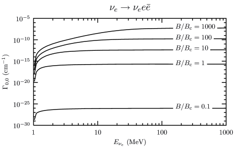
(a) Incoming electron neutrino

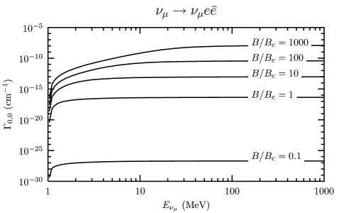
(b) Incoming muon (tau) neutrino

Figure 2: Production rates for the $n_{1}\,,n_{2}=0$ Landau levels where $\Gamma$ is the rate of production, $E_{\nu}$ is the energy of the incoming neutrino, and the magnetic field is measured relative to the critical field $B_{\mathrm{c}}=4.414\times 10^{13}~{}\mathrm{G}$. All plots are for a neutrino that is perpendicularly incident to the magnetic field.

Figure 3: The production rate’s dependance on the direction of the incoming neutrino.. The production rate is for the $0,0$ Landau level with an electron of energy $E_{\nu}=20m_{e}$ traveling at an angle $\theta$ relative to a magnetic field of strength equal to the critical field $B=B_{\mathrm{c}}$. Data is included for both an incoming electron-type neutrino (solid line) and a muon-type neutrino (dashed line). If we average over $\theta$, then the average production rate is $1.38\times 10^{-16}~{}\mathrm{cm}^{-1}$ for electron-type neutrinos or $2.94\times 10^{-17}~{}\mathrm{cm}^{-1}$ for muon or tau-type.

For comparison purposes, the production rates for other combinations of Landau levels have been calculated. These include the $1,0$ and $0,1$ cases (FIG. 4), the $20,0$ and $0,20$ cases (FIG. 5), and the $10,10$ case (FIG. 6). The first noteworthy feature of these results is that the production rates are decreasing at higher Landau levels. Because the energy required to create the pair goes as

$$E_{\mathrm{pair}} = E_{n_{1}}+E_{n_{2}}$$

$$= \sqrt{p_{1\,z}^{2}+2n_{1}eB+m_{e}^{2}}+\sqrt{p_{2\,z}^{2}+2n_{2}eB+m_{e}^{2}}$$

$$E_{\mathrm{pair}} \geq \sqrt{2n_{1}eB+m_{e}^{2}}+\sqrt{2n_{2}eB+m_{e}^{2}}\,,$$

the available phase space for the process should decrease in the order $0,0\ \to\ 0,1\ \to\ 0,20\ \to\ 10,10$. And as can be seen in FIGS. 2, 4, 5, and 6, the production rates fall off accordingly.

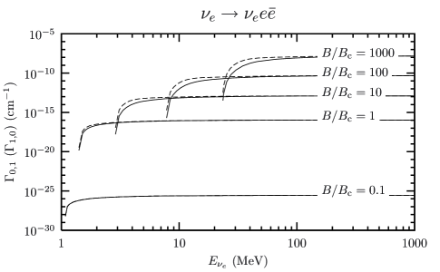
(a) Incoming electron neutrino

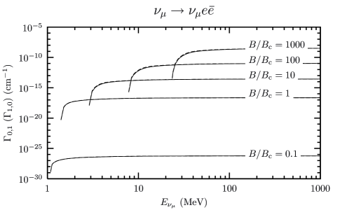
(b) Incoming muon neutrino

Figure 4: Production rates for the $n_{1}=0\,,n_{2}=1$ (solid) and $n_{1}=1\,,n_{2}=0$ (dashed) Landau levels where $\Gamma$ is the rate of production, $E_{\nu}$ is the energy of the incoming neutrino, and the magnetic field is measured relative to the critical field $B_{\mathrm{c}}=4.414\times 10^{13}~{}\mathrm{G}$.

Another interesting feature of these results is the apparent preference for the creation of electrons in the highest of the two Landau levels. That is, the rate of production is larger for the state $n_{1}=i\,,n_{2}=0$ than for $n_{1}=0\,,n_{2}=i$ (FIGS. 4 and 5). This behavior is especially significant over the range of incoming neutrino energies near its threshold value for creating pairs in the given states. Though the $i,0$ production rate is larger and increases more quickly in this “near-threshold” range than its $0,i$ counterpart, both curves plateau at higher energies, and their difference approaches zero. This difference is presumably caused by the positron having to share the $W$’s energy with the final electron-type neutrino. This also explains why such an effect is not seen for muon and tau-type neutrinos that only proceed through the neutral current reaction.

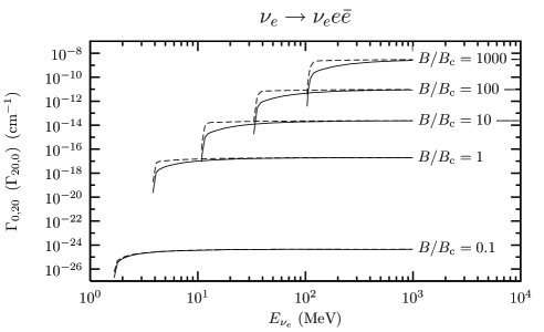
(a) Incoming electron neutrino

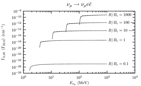
(b) Incoming muon neutrino

Figure 5: Production rates for the $n_{1}=0\,,n_{2}=20$ (solid) and $n_{1}=20\,,n_{2}=0$ (dashed) Landau levels where $\Gamma$ is the rate of production, $E_{\nu}$ is the energy of the incoming neutrino, and the magnetic field is measured relative to the critical field $B_{\mathrm{c}}=4.414\times 10^{13}~{}\mathrm{G}$.

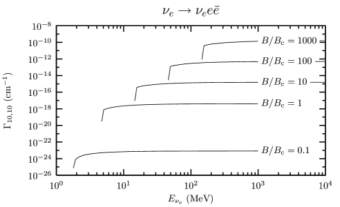
(a) Incoming electron neutrino

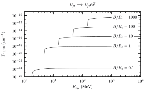
(b) Incoming muon neutrino

Figure 6: Production rates for the $n_{1}\,,n_{2}=10$ Landau levels where $\Gamma$ is the rate of production, $E_{\nu}$ is the energy of the incoming neutrino, and the magnetic field is measured relative to the critical field $B_{\mathrm{c}}=4.414\times 10^{13}~{}\mathrm{G}$.

It was mentioned in section I that previous authors have considered this process under two limiting cases Kuznetsov and Mikheev (1997). One is when the square of the energy of the initial-state neutrino and the magnetic field strength satisfy the conditions $E_{\nu}\gg eB\gg m_{e}^{2}$. Under these conditions many possible Landau levels could be stimulated, offering a multitude of production modes. Therefore, it would be inappropriate to compare their expression to our results for a specific set of Landau levels. However, the second limiting case is for $eB>E_{\nu}^{2}\gg m_{e}^{2}$. This condition is slightly more restrictive than our condition for the energies below which only the lowest energy Landau levels are occupied (Eq. (61)). In this regime our results for the $0,0$ state are the total production rates, and we can compare our results to the expression derived by the previous authors Kuznetsov and Mikheev (1997)

$$\Gamma=\frac{G_{F}^{2}\left({G_{V}^{\pm}}^{2}+1\right)}{2^{6}\pi^{3}}\,eB\,E_{\nu}^{3}\,\left(1+\mathcal{O}\left(E^{2}/eB\right)\right)\,,$$ (62)

where we have taken the direction of the incoming neutrino to be perpendicular to the magnetic field’s direction. Results of this comparison are shown in FIG. 7.

The results in FIG. 7 demonstrate the drawbacks of using the approximation in Eq. (62). While the expression is very simple, it gives only reasonable agreement with the production rate at a magnetic field equal to 100 times that of the critical field ($B=100\,B_{\mathrm{c}}$). Here it overestimates, at the very least, by a factor of two, and the inclusion of higher order corrections makes no significant improvement. One reason for the disagreement at this field strength is that there is only a very small range of energies that satisfy the condition $eB>E_{\nu}^{2}\gg m_{e}^{2}$. Therefore at higher field strengths we should get better agreement, and we do. Closer inspection of FIG. 7 reveals that the differences are less than a factor of three for neutrino energies in the range $2~{}\mathrm{MeV}<E_{\nu}<20~{}\mathrm{MeV}$, and the expression successfully provides a good order of magnitude estimation. Though the estimate will improve at higher magnetic field strengths, it begins to loose relevance as there are only a handful of known objects (namely magnetars) that can conceivably possess fields as high as $10^{15}$ G. Even for these objects, fields stronger than $10^{15}$ G cause instability in the star and the field begins to diminish Thompson and Duncan (1993).

(a) Incoming electron neutrino

(b) Incoming muon neutrino

Figure 7: The total production rate (solid lines) and its approximation (dashed lines)Kuznetsov and Mikheev (1997) for energies and magnetic field satisfying the condition $E_{\nu}^{2}<eB$. $E_{\nu}$ is the energy of the incoming neutrino, $m_{e}$ is the mass of the electron, and the magnetic field is measured relative to the critical field $B_{\mathrm{c}}=4.414\times 10^{13}~{}\mathrm{G}$.

Probing the limiting case $E_{\nu}\gg\sqrt{eB}$ is imperative because our present work has already demonstrated nontrivial deviation from approximate methods for realistic astrophysical magnetic field strengths and neutrino energies near and below the value $\sqrt{eB}$. But, as was mentioned previously, the number of Landau level states which contribute to the total production rate grows very rapidly in this higher energy regime, and we need to sum over these states. Future work will attempt to do these sums by using an approximation routine that can interpolate between rates for known sets of Landau levels. This will provide a flexible way to balance accuracy with computation time while determining when the production rate deviates from its limiting behavior. The significance of these deviations will only be known when a more complete understanding of the role that neutrino processes play in events such as supernova core-collapse and in the formation of the resulting neutron star. This work aims to improve that understanding.

Appendix A Calculation of $\mathbf{I_{n,m}}$

In section III.2 we discuss the fact that the squared scattering amplitude has coefficients that are integrals over the space-time coordinate $y$

$$I_{n,m}=\int\mathrm{d}y\,e^{i(p_{y}-p^{\prime}_{y})y}\,I_{n}(\xi_{-,1})\,I_{m}(\xi_{+,2})\,.$$ (63)

In this appendix we will derive the result after integrating over $y$.

By defining new parameters

$$\zeta = \sqrt{eB}\,y$$ (64)

$$\zeta_{i} = p_{ix}/\sqrt{eB}$$ (65)

$$\zeta_{0} = (p_{y}-p^{\prime}_{y})/\sqrt{eB}$$ (66)

and using the definition of $\xi$ (Eq. (11)) we can make a change of variable from $y$ to $\zeta$ and rewrite $I_{n,m}$ as

$$I_{n,m}=\int_{-\infty}^{\infty}\frac{\mathrm{d}\zeta}{\sqrt{eB}}\,e^{i\zeta_{0}\zeta}\,I_{n}(\zeta-\zeta_{1})\,I_{m}(\zeta+\zeta_{2})$$ (67)

where the limits of integration are $\pm\infty$ because we have taken the limit of $L_{y}$ as it approaches $\infty$. The $I_{n}(\xi)$ in Eq. (10) depend on the Hermite polynomials $H_{n}(\xi)$, which can be represented as a contour integral in the following way (Arfken and Weber, 1995, Eq. (13.8))

$$H_{n}(\xi)=\frac{n!}{2\pi i}\oint\mathrm{d}t\,t^{-n-1}\,e^{-t^{2}+2tx}\,.$$ (68)

Substituting this definition of the Hermite polynomial into Eq. (10) allows us to write the $I_{n,m}$ as

$$I_{n,m} = \int_{-\infty}^{\infty}\frac{\mathrm{d}\zeta}{\sqrt{eB}}\,e^{i\zeta_{0}\,\zeta}\,\left(\frac{\sqrt{eB}}{2^{n}\,n!\,\sqrt{\pi}}\right)^{1/2}e^{-(\zeta-\zeta_{1})^{2}/2}\,H_{n}(\zeta-\zeta_{1})\left(\frac{\sqrt{eB}}{2^{m}\,m!\,\sqrt{\pi}}\right)^{1/2}e^{-(\zeta+\zeta_{2})^{2}/2}\,H_{m}(\zeta+\zeta_{2})$$ (69)

$$= \left(2^{n+m}\,n!\,m!\,\pi\right)^{-1/2}\,\int_{-\infty}^{\infty}\mathrm{d}\zeta\,e^{i\zeta_{0}\,\zeta}\,e^{-(\zeta-\zeta_{1})^{2}/2}\,H_{n}(\zeta-\zeta_{1})e^{-(\zeta+\zeta_{2})^{2}/2}\,H_{m}(\zeta+\zeta_{2})$$

$$= \left(2^{n+m}\,n!\,m!\,\pi\right)^{-1/2}\,\int_{-\infty}^{\infty}\mathrm{d}\zeta\,e^{i\zeta_{0}\,\zeta}\,e^{-(\zeta-\zeta_{1})^{2}/2}\,e^{-(\zeta+\zeta_{2})^{2}/2}$$

$$\times\,\frac{n!}{2\pi i}\oint\mathrm{d}t\,t^{-n-1}\,e^{-t^{2}+2t(\zeta-\zeta_{1})}\frac{m!}{2\pi i}\oint\mathrm{d}s\,s^{-m-1}\,e^{-s^{2}+2s(\zeta+\zeta_{2})}\,.$$

Next, we isolate all of the $\zeta$ dependence, interchange the order of the integrals, and perform the integration over $\zeta$

$$\mathrm{Int}_{1} = \int_{-\infty}^{\infty}\mathrm{d}\zeta\,\exp\left(-\zeta^{2}+\zeta(\zeta_{1}-\zeta_{2}+i\zeta_{0}+2t+2s)\right)$$ (70)

$$= \sqrt{\pi}\ \exp\left(\left(\zeta_{1}-\zeta_{2}+i\zeta_{0}+2t+2s\right)^{2}/4\right)\,.$$

Substitution of this result back into Eq. (69) gives

$$I_{n,m} = \left(2^{n+m}\,n!\,m!\right)^{-1/2}\,e^{-\left((\zeta_{1}+\zeta_{2})^{2}+\zeta_{0}^{2}\right)/4}\,e^{i\zeta_{0}(\zeta_{1}-\zeta_{2})/2}$$

$$\times\,\frac{n!}{2\pi i}\oint\mathrm{d}t\,t^{-n-1}\,e^{t(-\zeta_{1}-\zeta_{2}+i\zeta_{0})}\,\frac{m!}{2\pi i}\oint\mathrm{d}s\,s^{-m-1}\,e^{s(\zeta_{1}+\zeta_{2}+i\zeta_{0})}\,e^{2st}\,.$$

If $m\geq n$, then we can perform the integration over $s$ first

$$\mathrm{Int}_{2} = \frac{m!}{2\pi i}\oint\mathrm{d}s\,s^{-m-1}\,e^{s(\zeta_{1}+\zeta_{2}+i\zeta_{0})}\,e^{2st}\,.$$ (72)

$$= \left.\frac{\mathrm{d}^{m}}{\mathrm{d}s^{m}}\,e^{s(\zeta_{1}+\zeta_{2}+i\zeta_{0}+2t)}\right|_{s=0}\,$$

$$= (\zeta_{1}+\zeta_{2}+i\zeta_{0}+2t)^{m}\,,$$

such that

$$I_{n,m} = \left(2^{n+m}\,n!\,m!\right)^{-1/2}\,\exp\left(-\left((\zeta_{1}+\zeta_{2})^{2}+\zeta_{0}^{2}\right)/4\right)\,\exp\left(i\zeta_{0}(\zeta_{1}-\zeta_{2})/2\right)$$ (73)

$$\times\,\frac{n!}{2\pi i}\oint\mathrm{d}t\,\frac{(\zeta_{1}+\zeta_{2}+i\zeta_{0}+2t)^{m}}{t^{n+1}}\,\exp\left(t(-\zeta_{1}-\zeta_{2}+i\zeta_{0})\right)\,.$$

The integration over $t$ is made easier by making the following changes of variable

$$\eta_{x} = \frac{\zeta_{1}+\zeta_{2}}{\sqrt{2}}\ =\ \frac{p_{1x}+p_{2x}}{\sqrt{2eB}}$$ (74)

$$\eta_{y} = \frac{\zeta_{0}}{\sqrt{2}}\ =\ \frac{p_{y}-p_{y}^{\prime}}{\sqrt{2eB}}$$ (75)

$$\phi_{0} = \frac{\zeta_{0}\,(\zeta_{1}-\zeta_{2})}{2}\ =\ \frac{(p_{y}-p_{y}^{\prime})(p_{1}-p_{2})}{2eB}$$ (76)

$$\eta^{\pm} = \eta_{x}\pm i\eta_{y}$$ (77)

$$\eta^{2} = \eta^{+}\,\eta^{-}\ =\ \eta_{x}^{2}+\eta_{y}^{2}$$ (78)

$$t = \left(u-\eta^{+}\right)/\sqrt{2}\,.$$ (79)

The integration over the variable $t$ can now be written as

$$\mathrm{Int}_{3} = \frac{n!}{2\pi i}\oint\frac{\mathrm{d}u}{\sqrt{2}}\,\frac{(\sqrt{2}\,u)^{m}}{\left(\left(u-\eta^{+}\right)/\sqrt{2}\right)^{n+1}}\,e^{\left((u-\eta^{+})/\sqrt{2}\right)(-\sqrt{2}\eta^{-})}$$

$$= 2^{(n+m)/2}\,e^{\eta^{2}}\,\frac{n!}{2\pi i}\oint\mathrm{d}u\,\frac{u^{m}}{\left(u-\eta^{+}\right)^{n+1}}\,e^{-u\eta^{-}}$$

$$= 2^{(n+m)/2}\,e^{\eta^{2}}\,\left.\frac{\mathrm{d}^{n}}{{\mathrm{d}u}^{n}}\,u^{m}\,e^{-u\eta^{-}}\right|_{u=\eta^{+}}$$

$$= 2^{(n+m)/2}\,e^{\eta^{2}}\,(\eta^{-})^{n-m}\frac{\mathrm{d}^{n}}{{\mathrm{d}(\eta^{2})}^{n}}\,(\eta^{2})^{m}\,e^{-\eta^{2}}$$

$$= n!\,2^{(n+m)/2}\,(\eta^{+})^{(m-n)}\,L^{m-n}_{n}(\eta^{2})$$

where we have used the Rodrigues’ representation for Laguerre polynomials (Arfken and Weber, 1995, Eq. (13.47))

$$L^{k}_{n}(x)=\frac{e^{x}\,x^{-k}}{n!}\,\frac{\mathrm{d}^{n}}{\mathrm{d}x^{n}}\,x^{n+k}\,e^{-x}\,,\qquad n,k\geq 0\,.$$ (80)

With the result from Eq. (A), we can now express the $I_{n,m}$ as

$$I_{n,m}=\sqrt{\frac{n!}{m!}}\ e^{-\eta^{2}/2}\,e^{i\phi_{0}}\,\left(\eta_{x}+i\,\eta_{y}\right)^{m-n}\,L_{n}^{m-n}(\eta^{2})\,,\quad m\geq n\geq 0\,,$$ (81)

For the case when $n>m$ we first integrate over $t$ in Eq. (A) and follow a similar procedure to find

$$I_{n,m}=\sqrt{\frac{m!}{n!}}\ e^{-\eta^{2}/2}\,e^{i\phi_{0}}\,\left(-\eta_{x}+i\,\eta_{y}\right)^{n-m}\,L_{m}^{n-m}(\eta^{2})\,,\quad n\geq m\geq 0\,.$$ (82)

Appendix B Result of trace

We can express the trace result for the average of the squared scattering amplitude from from Eq. (III.2) as a sum of terms

$$\overline{\left|\mathcal{M}\right|^{2}}=\frac{G_{F}^{2}}{2^{9}EE^{\prime}E_{n_{1}}E_{n_{2}}}\ \sum_{i=1}^{16}A_{i}\,\mathrm{T}_{i}\,,$$ (83)

where the coefficients $A_{i}$ depend on the products of $I_{n,m}$ and $I^{\ast}_{n^{\prime},m^{\prime}}$ defined in Eq. (47) and presented in appendix A, and the $T_{i}$ are the parts that depend on the contraction of the traces in Eq. (III.2). The results are as follows:

$$A_{1} = I_{n_{1},n_{2}}I^{\ast}_{n_{1},n_{2}}$$ (84)

$$T_{1} = \mathrm{Tr}\Bigl{\{}\gamma^{\sigma}\left(G_{V}^{\pm}-\gamma^{5}\right)\left[m(1-\sigma^{3})+\not\!{p}_{1\parallel}+\not\!{q}_{1\parallel}\gamma^{5}\right]\gamma^{\mu}\left(G_{V}^{\pm}-\gamma^{5}\right)\left[-m(1-\sigma^{3})+\not\!{p}_{2\parallel}+\not\!{q}_{2\parallel}\gamma^{5}\right]\Bigr{\}}$$

$$T_{1} = -2^{7}\left({G_{V}^{\pm}}^{2}-1\right)m_{e}^{2}\left(p_{x}p_{x}^{\prime}+p_{y}p_{y}^{\prime}\right)+2^{6}\left(G_{V}^{\pm}+1\right)^{2}(E-p_{z})(E^{\prime}-p_{z}^{\prime})(E_{n_{1}}+p_{1\,z})(E_{n_{2}}+p_{2\,z})$$ (85)

$$+2^{6}\left(G_{V}^{\pm}-1\right)^{2}(E+p_{z})(E^{\prime}+p_{z}^{\prime})(E_{n_{1}}-p_{1\,z})(E_{n_{2}}-p_{2\,z})$$

$$A_{2} = I_{n_{1},n_{2}-1}I^{\ast}_{n_{1},n_{2}}$$ (86)

$$T_{2} = \mathrm{Tr}\Bigl{\{}\gamma^{\sigma}\left(G_{V}^{\pm}-\gamma^{5}\right)\left[m(1-\sigma^{3})+\not\!{p}_{1\parallel}+\not\!{q}_{1\parallel}\gamma^{5}\right]\gamma^{\mu}\left(G_{V}^{\pm}-\gamma^{5}\right)(-\sqrt{2n_{2}eB})\left(\gamma^{1}+i\gamma^{2}\right)\Bigr{\}}$$

$$T_{2} = -2^{6}\left(G_{V}^{\pm}+1\right)^{2}\sqrt{2n_{2}eB}\,(p_{x}+i\,p_{y})(E^{\prime}-p_{z}^{\prime})(E_{n_{1}}+p_{1\,z})$$ (87)

$$-2^{6}\left(G_{V}^{\pm}-1\right)^{2}\sqrt{2n_{2}eB}\,(p_{x}^{\prime}+i\,p_{y}^{\prime})(E+p_{z})(E_{n_{1}}-p_{1\,z})$$

$$A_{3} = I_{n_{1},n_{2}}I^{\ast}_{n_{1},n_{2}-1}\ =\ A^{\ast}_{2}$$ (88)

$$T_{3} = T^{\ast}_{2}$$ (89)

$$A_{4} = I_{n_{1},n_{2}-1}I^{\ast}_{n_{1},n_{2}-1}$$ (90)

$$T_{4} = \mathrm{Tr}\Bigl{\{}\gamma^{\sigma}\left(G_{V}^{\pm}-\gamma^{5}\right)\left[m(1-\sigma^{3})+\not\!{p}_{1\parallel}+\not\!{q}_{1\parallel}\gamma^{5}\right]\gamma^{\mu}\left(G_{V}^{\pm}-\gamma^{5}\right)\left[-m(1+\sigma^{3})+\not\!{p}_{2\parallel}-\not\!{q}_{2\parallel}\gamma^{5}\right]\Bigr{\}}$$

$$T_{4} = 2^{7}\left({G_{V}^{\pm}}^{2}-1\right)m_{e}^{2}(E+p_{z})(E^{\prime}-p_{z}^{\prime})+2^{6}\left(G_{V}^{\pm}+1\right)^{2}(E+p_{z})(E^{\prime}-p_{z}^{\prime})(E_{n_{1}}+p_{1\,z})(E_{n_{2}}-p_{2\,z})$$ (91)

$$+2^{6}\left(G_{V}^{\pm}-1\right)^{2}(E+p_{z})(E^{\prime}-p_{z}^{\prime})(E_{n_{1}}-p_{1\,z})(E_{n_{2}}+p_{2\,z})$$

$$A_{5} = I_{n_{1},n_{2}}I^{\ast}_{n_{1}-1,n_{2}}$$ (92)

$$T_{5} = \mathrm{Tr}\Bigl{\{}\gamma^{\sigma}\left(G_{V}^{\pm}-\gamma^{5}\right)(\sqrt{2n_{1}eB})\left(\gamma^{1}+i\gamma^{2}\right)\gamma^{\mu}\left(G_{V}^{\pm}-\gamma^{5}\right)\left[-m(1-\sigma^{3})+\not\!{p}_{2\parallel}+\not\!{q}_{2\parallel}\gamma^{5}\right]\Bigr{\}}$$

$$T_{5} = 2^{6}\left(G_{V}^{\pm}+1\right)^{2}\sqrt{2n_{1}eB}\,(p_{x}^{\prime}+i\,p_{y}^{\prime})(E-p_{z})(E_{n_{2}}+p_{2\,z})$$ (93)

$$+2^{6}\left(G_{V}^{\pm}-1\right)^{2}\sqrt{2n_{1}eB}\,(p_{x}+i\,p_{y})(E^{\prime}+p_{z}^{\prime})(E_{n_{2}}-p_{2\,z})$$

$$A_{6} = I_{n_{1},n_{2}-1}I^{\ast}_{n_{1}-1,n_{2}}$$ (94)

$$T_{6} = \mathrm{Tr}\Bigl{\{}\gamma^{\sigma}\left(G_{V}^{\pm}-\gamma^{5}\right)(\sqrt{2n_{1}eB})\left(\gamma^{1}+i\gamma^{2}\right)\gamma^{\mu}\left(G_{V}^{\pm}-\gamma^{5}\right)(-\sqrt{2n_{2}eB})\left(\gamma^{1}+i\gamma^{2}\right)\Bigr{\}}$$

$$T_{6} = -2^{6}\left(G_{V}^{\pm}+1\right)^{2}\sqrt{2n_{1}eB}\,\sqrt{2n_{2}eB}\,(p_{x}+i\,p_{y})(p_{x}^{\prime}+i\,p_{y}^{\prime})$$ (95)

$$-2^{6}\left(G_{V}^{\pm}-1\right)^{2}\sqrt{2n_{1}eB}\,\sqrt{2n_{2}eB}\,(p_{x}+i\,p_{y})(p_{x}^{\prime}+i\,p_{y}^{\prime})$$

$$A_{7} = I_{n_{1},n_{2}}I^{\ast}_{n_{1}-1,n_{2}-1}$$ (96)

$$T_{7} = \mathrm{Tr}\Bigl{\{}\gamma^{\sigma}\left(G_{V}^{\pm}-\gamma^{5}\right)(\sqrt{2n_{1}eB})\left(\gamma^{1}+i\gamma^{2}\right)\gamma^{\mu}\left(G_{V}^{\pm}-\gamma^{5}\right)(-\sqrt{2n_{2}eB})\left(\gamma^{1}-i\gamma^{2}\right)\Bigr{\}}$$

$$T_{7} = -2^{6}\left(G_{V}^{\pm}+1\right)^{2}\sqrt{2n_{1}eB}\,\sqrt{2n_{2}eB}\,(p_{x}-i\,p_{y})(p_{x}^{\prime}+i\,p_{y}^{\prime})$$ (97)

$$-2^{6}\left(G_{V}^{\pm}-1\right)^{2}\sqrt{2n_{1}eB}\,\sqrt{2n_{2}eB}\,(p_{x}+i\,p_{y})(p_{x}^{\prime}-i\,p_{y}^{\prime})$$

$$A_{8} = I_{n_{1},n_{2}-1}I^{\ast}_{n_{1}-1,n_{2}-1}$$ (98)

$$T_{8} = \mathrm{Tr}\Bigl{\{}\gamma^{\sigma}\left(G_{V}^{\pm}-\gamma^{5}\right)(\sqrt{2n_{1}eB})\left(\gamma^{1}+i\gamma^{2}\right)\gamma^{\mu}\left(G_{V}^{\pm}-\gamma^{5}\right)\left[-m(1+\sigma^{3})+\not\!{p}_{2\parallel}-\not\!{q}_{2\parallel}\gamma^{5}\right]\Bigr{\}}$$

$$T_{8} = 2^{6}\left(G_{V}^{\pm}+1\right)^{2}\sqrt{2n_{1}eB}\,(p_{x}^{\prime}+i\,p_{y}^{\prime})(E+p_{z})(E_{n_{2}}-p_{2\,z})$$ (99)

$$+2^{6}\left(G_{V}^{\pm}-1\right)^{2}\sqrt{2n_{1}eB}\,(p_{x}+i\,p_{y})(E^{\prime}+p_{z}^{\prime})(E_{n_{2}}+p_{2\,z})$$

$$A_{9} = I_{n_{1}-1,n_{2}}I^{\ast}_{n_{1},n_{2}}\ =\ A_{5}^{\ast}$$ (100)

$$T_{9} = T_{5}^{\ast}$$ (101)

$$A_{10} = I_{n_{1}-1,n_{2}-1}I^{\ast}_{n_{1},n_{2}}\ =\ A_{7}$$ (102)

$$T_{10} = T_{7}^{\ast}$$ (103)

$$A_{11} = I_{n_{1},n_{2}}I^{\ast}_{n_{1},n_{2}-1}\ =\ A^{\ast}_{6}$$ (104)

$$T_{11} = T^{\ast}_{6}$$ (105)

$$A_{12} = I_{n_{1}-1,n_{2}-1}I^{\ast}_{n_{1},n_{2}-1}\ =\ A_{8}^{\ast}$$ (106)

$$T_{12} = T_{8}^{\ast}$$ (107)

$$A_{13} = I_{n_{1}-1,n_{2}}I^{\ast}_{n_{1}-1,n_{2}}$$ (108)

$$T_{13} = \mathrm{Tr}\Bigl{\{}\gamma^{\sigma}\left(G_{V}^{\pm}-\gamma^{5}\right)\left[m(1+\sigma^{3})+\not\!{p}_{1\parallel}-\not\!{q}_{1\parallel}\gamma^{5}\right]\gamma^{\mu}\left(G_{V}^{\pm}-\gamma^{5}\right)\left[-m(1-\sigma^{3})+\not\!{p}_{2\parallel}+\not\!{q}_{2\parallel}\gamma^{5}\right]\Bigr{\}}$$

$$T_{13} = 2^{7}\left({G_{V}^{\pm}}^{2}-1\right)m_{e}^{2}(E-p_{z})(E^{\prime}+p_{z}^{\prime})+2^{6}\left(G_{V}^{\pm}+1\right)^{2}(E-p_{z})(E^{\prime}+p_{z}^{\prime})(E_{n_{1}}-p_{1\,z})(E_{n_{2}}+p_{2\,z})$$ (109)

$$+2^{6}\left(G_{V}^{\pm}-1\right)^{2}(E-p_{z})(E^{\prime}+p_{z}^{\prime})(E_{n_{1}}+p_{1\,z})(E_{n_{2}}-p_{2\,z})$$

$$A_{14} = I_{n_{1}-1,n_{2}-1}I^{\ast}_{n_{1}-1,n_{2}}$$ (110)

$$T_{14} = \mathrm{Tr}\Bigl{\{}\gamma^{\sigma}\left(G_{V}^{\pm}-\gamma^{5}\right)\left[m(1+\sigma^{3})+\not\!{p}_{1\parallel}-\not\!{q}_{1\parallel}\gamma^{5}\right]\gamma^{\mu}\left(G_{V}^{\pm}-\gamma^{5}\right)(-\sqrt{2n_{2}eB})\left(\gamma^{1}+i\gamma^{2}\right)\Bigr{\}}$$

$$T_{14} = -2^{6}\left(G_{V}^{\pm}+1\right)^{2}(\sqrt{2n_{2}eB})(p_{x}+ip_{y})(E^{\prime}+p_{z}^{\prime})(E_{n_{1}}-p_{1\,z})$$ (111)

$$-2^{6}\left(G_{V}^{\pm}-1\right)^{2}(\sqrt{2n_{2}eB})(p_{x}^{\prime}+ip_{y}^{\prime})(E-p_{z})(E_{n_{1}}+p_{1\,z})$$

$$A_{15} = I_{n_{1}-1,n_{2}}I^{\ast}_{n_{1}-1,n_{2}-1}\ =\ A^{\ast}_{14}$$ (112)

$$T_{15} = T_{14}^{\ast}$$ (113)

$$A_{16} = I_{n_{1}-1,n_{2}-1}I^{\ast}_{n_{1}-1,n_{2}-1}$$ (114)

$$T_{16} = \mathrm{Tr}\Bigl{\{}\gamma^{\sigma}\left(G_{V}^{\pm}-\gamma^{5}\right)\left[m(1+\sigma^{3})+\not\!{p}_{1\parallel}-\not\!{q}_{1\parallel}\gamma^{5}\right]\gamma^{\mu}\left(G_{V}^{\pm}-\gamma^{5}\right)\left[-m(1+\sigma^{3})+\not\!{p}_{2\parallel}-\not\!{q}_{2\parallel}\gamma^{5}\right]\Bigr{\}}$$

$$T_{16} = -2^{7}\left({G_{V}^{\pm}}^{2}-1\right)m_{e}^{2}(p_{x}p_{x}^{\prime}+p_{y}p_{y}^{\prime})+2^{6}\left(G_{V}^{\pm}+1\right)^{2}(E+p_{z})(E^{\prime}+p_{z}^{\prime})(E_{n_{1}}-p_{1\,z})(E_{n_{2}}-p_{2\,z})$$ (115)

$$+2^{6}\left(G_{V}^{\pm}-1\right)^{2}(E-p_{z})(E^{\prime}-p_{z}^{\prime})(E_{n_{1}}+p_{1\,z})(E_{n_{2}}+p_{2\,z})\,.\quad$$