Effect of atomic beam alignment on photon correlation measurements
in cavity QED

Abstract

Quantum trajectory simulations of a cavity QED system comprising an atomic beam traversing a standing-wave cavity are carried out. The delayed photon coincident rate for forwards scattering is computed and compared with the measurements of Rempe et al. [Phys. Rev. Lett. 67, 1727 (1991)] and Foster et al. [Phys. Rev. A 61, 053821 (2000)]. It is shown that a moderate atomic beam misalignment can account for the degradation of the predicted correlation. Fits to the experimental data are made in the weak-field limit with a single adjustable parameter—the atomic beam tilt from perpendicular to the cavity axis. Departures of the measurement conditions from the weak-field limit are discussed.

I Introduction

Cavity quantum electrodynamics Berman (1994); Raimond et al. (2001); Mabuchi and Doherty (2002); Vahala (2003); Khitrova et al. (2006); Carmichael (2007) has as its central objective the realization of strong dipole coupling between a discrete transition in matter (e.g., an atom or quantum dot) and a mode of an electromagnetic cavity. Most often strong coupling is demonstrated through the realization of vacuum Rabi splitting Sanchez-Mondragon et al. (1983); Agarwal (1984). First realized for Rydberg atoms in superconducting microwave cavities Bernardot et al. (1992); Brune et al. (1996) and for transitions at optical wavelengths in high-finesse Fabry Perots Thompson et al. (1992); Childs et al. (1996); Boca et al. (2004); Maunz et al. (2005), vacuum Rabi splitting was recently observed in monolithic structures where the discrete transition is provided by a semiconductor quantum dot Yoshie et al. (2004); Reithmaier et al. (2004); Peter et al. (2005), and in a coupled system of qubit and resonant circuit engineered from superconducting electronics Wallraff et al. (2004).

More generally, vacuum Rabi spectra can be observed for any pair of coupled harmonic oscillators Car (a) without the need for strong coupling of the one-atom kind. Prior to observations for single atoms and quantum dots, similar spectra were observed in many-atom Raizen et al. (1989); Zhu et al. (1990); Gripp et al. (1996) and -exciton Weisbuch et al. (1992); Khitrova et al. (1999) systems where the radiative coupling is collectively enhanced.

The definitive signature of single-atom strong coupling is the large effect a single photon in the cavity has on the reflection, side-scattering, or transmission of another photon. Strong coupling has a dramatic effect, for example, on the delayed photon coincidence rate in forwards scattering when a cavity QED system is coherently driven on axis Carmichael (1985); Rice and Carmichael (1988); Carmichael et al. (1991); Brecha et al. (1999). Photon antibunching is seen at a level proportional to the parameter $2C_{1}=2g^{2}/\gamma\kappa$ Carmichael et al. (1991), where $g$ is the atomic dipole coupling constant, $\gamma$ is the atomic spontaneous emission rate, and $2\kappa$ is the photon loss rate from the cavity; the collective parameter $2C=N2C_{1}$, with $N$ the number of atoms, does not enter into the magnitude of the effect when $N\gg 1$. In the one-atom case, and for $2\kappa\gg\gamma$, the size of the effect is raised to $(2C_{1})^{2}$ Carmichael (1985); Rice and Carmichael (1988) [see Eq. (30)].

The first demonstration of photon antibunching was made Rempe et al. (1991) for moderately strong coupling ($2C_{1}\approx 4.6$) and $N=18$, $45$, and $110$ (effective) atoms. The measurement has subsequently been repeated for somewhat higher values of $2C_{1}$ and slightly fewer atoms Mielke et al. (1998); Foster et al. (2000a), and a measurement for one trapped atom Birnbaum et al. (2005), in a slightly altered configuration, has demonstrated the so-called photon blockade effect Imamoḡlu et al. (1979); Werner and Imamoḡlu (1999); Rebić et al. (1999, 2002); Kim et al. (1999); Smolyaninov et al. (2002)—i.e., the antibunching of forwards-scattered photons for coherent driving of a vacuum-Rabi resonance, in which case a two-state approximation may be made Tian and Carmichael (1992), assuming the coupling is sufficiently strong.

The early experiments of Rempe et al. Rempe et al. (1991) and those of Mielke et al. Mielke et al. (1998) and Foster et al. Foster et al. (2000a) employ systems designed around a Fabry-Perot cavity mode traversed by a thermal atomic beam. Their theoretical modeling therefore presents a significant challenge, since for the numbers of effective atoms used, the atomic beam carries hundreds of atoms—typically an order of magnitude larger than the effective number Carmichael and Sanders (1999)—into the interaction volume. The Hilbert space required for exact calculations is enormous ($2^{100}\sim 10^{30}$); it grows and shrinks with the number of atoms, which inevitably fluctuates over time; and the atoms move through a spatially varying cavity mode, so their coupling strengths are changing in time. Ideally, all of these features should be taken into account, although certain approximations might be made.

For weak excitation, as in the experiments, the lowest permissible truncation of the Hilbert space—when calculating two-photon correlations—is at the two-quanta level. Within a two-quanta truncation, relatively simple formulas can be derived so long as the atomic motion is overlooked Carmichael et al. (1991); Brecha et al. (1999). It is even possible to account for the unequal coupling strengths of different atoms, and, through a Monte-Carlo average, fluctuations in their spatial distribution Rempe et al. (1991). A significant discrepancy between theory and experiment nevertheless remains: Rempe et al. Rempe et al. (1991) describe how the amplitude of the Rabi oscillation (magnitude of the antibunching effect) was scaled down by a factor of 4 and a slight shift of the theoretical curve was made in order to bring their data into agreement with this model; the discrepancy persists in the experiments of Foster et al. Foster et al. (2000a), except that the required adjustment is by a scale factor closer to 2 than to 4.

Attempts to account for these discrepancies have been made but are unconvincing. Martini and Schenzle Martini and Schenzle (2001) report good agreement with one of the data sets from Ref. Rempe et al. (1991); they numerically solve a many-atom master equation, but under the unreasonable assumption of stationary atoms and equal coupling strengths. The unlikely agreement results from using parameters that are very far from those of the experiment—most importantly, the dipole coupling constant is smaller by a factor of approximately 3.

Foster et al. Foster et al. (2000a) report a rather good theoretical fit to one of their data sets. It is obtained by using the mentioned approximations and adding a detuning in the calculation to account for the Doppler broadening of a misaligned atomic beam. They state that “Imperfect alignment $\ldots$ can lead to a tilt from perpendicular of as much as $1^{\circ}$”. They suggest that the mean Doppler shift is offset in the experiment by adjusting the driving laser frequency and account for the distribution about the mean in the model. There does appear to be a difficulty with this procedure, however, since while such an offset should work for a ring cavity, it is unlikely to do so in the presence of the counter-propagating fields of a Fabry-Perot. Indeed, we are able to successfully simulate the procedure only for the ring-cavity case (Sec. IV.3).

The likely candidates to explain the disagreement between theory and experiment have always been evident. For example, Rempe et al. Rempe et al. (1991) state:

• “Apparently the transient nature of the atomic motion through the cavity mode (which is not included here or in Ref. [7]) has a profound effect in decorrelating the otherwise coherent response of the sample to the escape of a photon.”

and also:

• “Empirically, we also know that $|g^{(2)}(0)-1|$ is reduced somewhat because the weak-field limit is not strictly satisfied in our measurements.”

To these two observations we should add—picking up on the comment in Foster et al. (2000a)—that in a standing-wave cavity an atomic beam misalignment would make the decorrelation from atomic motion a great deal worse.

Thus, the required improvements in the modeling are: (i) a serious accounting for atomic motion in a thermal atomic beam, allowing for up to a few hundred interacting atoms and a velocity component along the cavity axis, and (ii) extension of the Hilbert space to include 3, 4, etc. quanta of excitation, thus extending the model beyond the weak-field limit. The first requirement is entirely achievable in a quantum trajectory simulation Carmichael (1993); Dalibard et al. (1992); Dum et al. (1992); Gardiner and Zoller (2004); Car (b), while the second, even with recent improvements in computing power, remains a formidable challenge.

In this paper we offer an explanation of the discrepancies between theory and experiment in the measurements of Refs. Rempe et al. (1991) and Foster et al. (2000a). We perform ab initio quantum trajectory simulations in parallel with a Monte-Carlo simulation of a tilted atomic beam. The parameters used are listed in Table 1: Set 1 corresponds to the data displayed in Fig. 4(a) of Ref. Rempe et al. (1991), and Set 2 to the data displayed in Fig. 4 of Ref. Foster et al. (2000a). All parameters are measured quantities— or are inferred from measured quantities—and the atomic beam tilt alone is varied to optimize the data fit. Excellent agreement is demonstrated for atomic beam misalignments of approximately $10\mkern 2.0mu{\rm mrad}$ (a little over $1/2^{\circ}$). These simulations are performed using a two-quanta truncation of the Hilbert space.

Simulations based upon a three-quanta truncation are also carried out, which, although not adequate for the experimental conditions, can begin to address physics beyond the weak-field limit. From these, an inconsistency with the intracavity photon number reported by Foster et al. Foster et al. (2000a) is found.

Parameter	Set $1$	Set $2$
cavity halfwidth $\mkern 45.0mu\kappa/2\pi$	$0.9\mkern 1.0mu{\rm MHz}$	$7.9\mkern 1.0mu{\rm MHz}$
dipole coupling constant $\mkern 70.0mug_{\rm max}/\kappa$	$3.56$	$1.47$
atomic linewidth $\mkern 50.0mu\gamma/\kappa$	$5.56$	$0.77$
mode waist $\mkern 33.0muw_{\rm 0}$	$50\mkern 1.0mu\mu{\rm m}$	$21.5\mkern 1.0mu\mu{\rm m}$
wavelength $\mkern 35.0mu\lambda$	$\mkern 5.0mu852{\rm nm}$ (Cs)	$\mkern 5.0mu780{\rm nm}$ (Rb)
effective atom number $\mkern 75.0mu\bar{N}_{\rm eff}$	18	13
oven temperature $\mkern 60.0muT$	$473\mkern 1.0mu{\rm K}$	$430\mkern 1.0mu{\rm K}$
mean speed in oven $\mkern 65.0mu\overline{v}_{\rm oven}$	$274.5\mkern 1.0mu{\rm m\!/s}$	$326.4\mkern 1.0mu{\rm m\!/s}$
mean speed in beam $\mkern 65.0mu\overline{v}_{\rm beam}$	$323.4\mkern 1.0mu{\rm m\!/s}$	$384.5\mkern 1.0mu{\rm m\!/s}$

Table 1: Parameters used in the simulations. Set 1 is taken from Ref. Rempe et al. (1991) and Set 2 from Ref. Foster et al. (2000a).

Our model is described in Sec. II, where we formulate the stochastic master equation used to describe the atomic beam, its quantum trajectory unraveling, and the two-quanta truncation of the Hilbert space. The previous modeling on the basis of a stationary-atom approximation is reviewed in Sect. III and compared with the data of Rempe et al. Rempe et al. (1991) and Foster et al. Foster et al. (2000a). The effects of atomic beam misalignment are discussed in Sec. IV; here the results of simulations with a two-quanta truncation are presented. Results obtained with a three-quanta truncation are presented in Sec. V, where the issue of intracavity photon number is discussed. Our conclusions are stated in Sec. VI.

II Cavity QED with Atomic Beams

II.1 Stochastic Master Equation: Atomic Beam Simulation

Thermal atomic beams have been used extensively for experiments in cavity QED Bernardot et al. (1992); Brune et al. (1996); Thompson et al. (1992); Childs et al. (1996); Raizen et al. (1989); Zhu et al. (1990); Gripp et al. (1996); Rempe et al. (1991); Mielke et al. (1998); Foster et al. (2000a). The experimental setups under consideration are described in detail in Refs. Brecha (1990) and Foster (1999). As typically, the beam is formed from an atomic vapor created inside an oven, from which atoms escape through a collimated opening. We work from the standard theory of an effusive source from a thin-walled oriface Ramsey (1956), for which for an effective number $\bar{N}_{\rm eff}$ of intracavity atoms Thompson et al. (1992); Carmichael and Sanders (1999) and cavity mode waist $\omega_{0}$ ($\bar{N}_{\rm eff}$ is the average number of atoms within a cylinder of radius $w_{0}/2$), the average escape rate is

$$R=64\bar{N}_{\rm eff}\bar{v}_{\rm beam}/3\pi^{2}w_{0},$$ (1)

with mean speed in the beam

$$\bar{v}_{\rm beam}=\sqrt{9\pi k_{B}T/8M},$$ (2)

where $k_{B}$ is Boltzmann’s constant, $T$ is the oven temperature, and $M$ is the mass of an atom; the beam has atomic density

$$\varrho=4\bar{N}_{\rm eff}/\pi w_{0}^{2}l,$$ (3)

where $l$ is the beam width, and distribution of atomic speeds

$$P(v)dv=2u^{3}(v)e^{-u^{2}(v)}du(v),$$ (4)

$u(v)\equiv 2v/\sqrt{\pi}\mkern 2.0mu\bar{v}_{\rm oven}$, where

$$\bar{v}_{\rm oven}=\sqrt{8k_{B}T/\pi M}=(8/3\pi)\bar{v}_{\rm beam}$$ (5)

is the mean speed of an atom inside the oven, as calculated from the Maxwell-Boltzmann distribution. Note that $\bar{v}_{\rm beam}$ is larger than $\bar{v}_{\rm oven}$ because those atoms that move faster inside the oven have a higher probability of escape.

In an open-sided cavity, neither the interaction volume nor the number of interacting atoms is well-defined; the cavity mode function and atomic density are the well-defined quantities. Clearly, though, as the atomic dipole coupling strength decreases with the distance of the atom from the cavity axis, those atoms located far away from the axis may be neglected, introducing, in effect, a finite interaction volume. How far from the cavity axis, however, is far enough? One possible criterion is to require that the interaction volume taken be large enough to give an accurate result for the collective coupling strength, or, considering its dependence on atomic locations (at fixed average density), the probability distribution over collective coupling strengths. According to this criterion, the actual number of interacting atoms is typically an order of magnitude larger than $\bar{N}_{\rm eff}$ Carmichael and Sanders (1999). If, for example, one introduces a cut-off parameter $F<1$, and defines the interaction volume by Carmichael and Sanders (1999); Carmichael et al. (1996); Sanders et al. (1997)

$$V_{F}\equiv\{(x,y,z):g(x,y,z)\geq Fg_{\rm max}\},$$ (6)

with

$$g(x,y,z)=g_{\rm max}\cos(kz)\exp\!\left[-(x^{2}+y^{2})/w_{0}^{2}\right]$$ (7)

the spatially varying coupling constant for a standing-wave TEM₀₀ cavity mode not —wavelength $\lambda=2\pi/k$—the computed collective coupling constant is Carmichael and Sanders (1999)

$$\sqrt{\bar{N}_{\rm eff}}\mkern 5.0mug_{\rm max}\to\sqrt{\bar{N}_{\rm eff}^{F}}\mkern 5.0mug_{\rm max},$$

with

$$\bar{N}_{\rm eff}^{F}=(2\bar{N}_{\rm eff}/\pi)\mkern-5.0mu\left[(1-2F^{2})\cos^{-1}F+F\sqrt{1-F^{2}}\right].$$ (8)

For the choice $F=0.1$, one obtains $\bar{N}_{\rm eff}^{F}=0.98\bar{N}_{\rm eff}$, a reduction of the collective coupling strength by 1%, and the interaction volume—radius $r\approx 3(w_{0}/2)$—contains approximately $9\bar{N}_{\rm eff}$ atoms on average. This is the choice made for the simulations with a three-quanta truncation reported in Sec. V. When adopting a two-quanta truncation, with its smaller Hilbert space for a given number of atoms, we choose $F=0.01$, which yields $\bar{N}_{\rm eff}^{F}=0.9998\bar{N}_{\rm eff}$ and $r\approx 4.3(w_{0}/2)$, and approximately $18\bar{N}_{\rm eff}$ atoms in the interaction volume on average.

In fact, the volume used in practice is a little larger than $V_{F}$. In the course of a Monte-Carlo simulation of the atomic beam, atoms are created randomly at rate $R$ on the plane $x=-w_{0}\sqrt{|\ln F|}$. At the time, $t_{0}^{j}$, of its creation, each atom is assigned a random position and velocity ($j$ labels a particular atom),

$${\bm{r}}_{j}(t_{0}^{j})=\mkern-3.0mu\left(\begin{matrix}-w_{0}\sqrt{|\ln F|}\\ \vskip 2.0pt\cr y_{j}(t_{0}^{j})\\ \vskip 3.0pt\cr z_{j}(t_{0}^{j})\end{matrix}\right),\qquad{\bm{v}_{j}}=v_{j}\mkern-3.0mu\left(\begin{matrix}\cos\theta\\ 0\\ \sin\theta\end{matrix}\right),$$ (9)

where $y_{j}(t_{0}^{j})$ and $z_{j}(t_{0}^{j})$ are random variables, uniformly distributed on the intervals $|y_{j}(t_{0}^{j})|\leq w_{0}\sqrt{|\ln F|}\mkern 2.0mu$ and $|z_{j}(t_{0}^{j})|\leq\lambda/4$, respectively, and $v_{j}$ is sampled from the distribution of atomic speeds [Eq. (4)]; $\theta$ is the tilt of the atomic beam away from perpendicular to the cavity axis. The atom moves freely across the cavity after its creation, passing out of the interaction volume on the plane $x=w_{0}\sqrt{|\ln F|}$. Thus the interaction volume has a square rather than circular cross section and measures $2\sqrt{|\ln F|}w_{0}$ on a side. It is larger than $V_{F}$ by approximately $30\%$.

Atoms are created in the ground state and returned to the ground state when they leave the interaction volume. On leaving an atom is disentangled from the system by comparing its probability of excitation with a uniformly distributed random number $r$, $0\leq r\leq 1$, and deciding whether or not it will—anytime in the future—spontaneously emit; thus, the system state is projected onto the excited state of the leaving atom (the atom will emit) or its ground state (it will not emit) and propagated forwards in time.

Note that the effects of light forces and radiative heating are neglected. At the thermal velocities considered, typically the ratio of kinetic energy to recoil energy is of order $10^{8}$, while the maximum light shift $\hbar g_{\rm max}$ (assuming one photon in the cavity) is smaller than the kinetic energy by a factor of $10^{7}$; even if the axial component of velocity only is considered, these ratios are as high as $10^{4}$ and $10^{3}$ with $\theta\sim 10\mkern 2.0mu{\rm mrad}$, as in Figs. 10 and 11. In fact, the mean intracavity photon number is considerably less than one (Sec. V); thus, for example, the majority of atoms traverse the cavity without making a single spontaneous emission.

Under the atomic beam simulation, the atom number, $N(t)$, and locations ${\bm{r}_{j}(t)}$, $j=1,\ldots,N(t)$, are changing in time; therefore, the atomic state basis is dynamic, growing and shrinking with $N(t)$. We assume all atoms couple resonantly to the cavity mode, which is coherently driven on resonance with driving field amplitude $\cal{E}$. Then, including spontaneous emission and cavity loss, the system is described by the stochastic master equation in the interaction picture

$$\dot{\rho} = {\cal E}[\hat{a}^{{\dagger}}-\hat{a},\rho]+\sum_{j=1}^{N(t)}g({\bm{r}}_{j}(t))[\hat{a}^{{\dagger}}\hat{\sigma}_{j-}-\hat{a}\hat{\sigma}_{j+},\rho]$$ (10)

$$+\frac{\gamma}{2}\sum_{j=1}^{N(t)}\left(2\hat{\sigma}_{j-}\rho\hat{\sigma}_{j+}-\hat{\sigma}_{j+}\hat{\sigma}_{j-}\rho-\rho\hat{\sigma}_{j+}\hat{\sigma}_{j-}\right)$$

$$+\kappa\left(2\hat{a}\rho\hat{a}^{{\dagger}}-\hat{a}^{{\dagger}}\hat{a}\rho-\rho\hat{a}^{{\dagger}}\hat{a}\right),$$

with dipole coupling constants

$$g({\bm{r}}_{j}(t))=g_{\rm max}\cos(kz_{j}(t))\exp\!\left[-\frac{x_{j}^{2}(t)+y_{j}^{2}(t)}{w_{0}^{2}}\right],$$ (11)

where $\hat{a}^{\dagger}$ and $\hat{a}$ are creation and annihilation operators for the cavity mode, and $\hat{\sigma}_{j+}$ and $\hat{\sigma}_{j-}$, $j=1\ldots N(t)$, are raising and lowering operators for two-state atoms.

II.2 Quantum Trajectory Unraveling

In principle, the stochastic master equation might be simulated directly, but it is impossible to do so in practice. Table 1 lists effective numbers of atoms $\bar{N}_{\rm eff}=18$ and $\bar{N}_{\rm eff}=13$. For cut-off parameter $F=0.01$ and an interaction volume of approximately $1.3\times V_{F}$ [see the discussion below Eq. (8)], an estimate of the number of interacting atoms gives $N(t)\sim 1.3\times 18\bar{N}_{\rm eff}\approx 420$ and $300$, respectively, which means that even in a two-quanta truncation the size of the atomic state basis ($\sim 10^{5}$ states) is far too large to work with density matrix elements. We therefore make a quantum trajectory unraveling of Eq. (10) Carmichael (1993); Dalibard et al. (1992); Dum et al. (1992); Gardiner and Zoller (2004); Car (b), where, given our interest in delayed photon coincidence measurements, conditioning of the evolution upon direct photoelectron counting records is appropriate: the (unnormalized) conditional state satisfies the nonunitary Schrödinger equation

$$\frac{d|\bar{\psi}_{\rm REC}\rangle}{dt}=\frac{1}{i\hbar}\hat{H}_{B}(t)|\bar{\psi}_{\rm REC}\rangle,$$ (12)

with non-Hermitian Hamiltonian

$$\hat{H}_{B}(t)/i\hbar = {\cal E}(\hat{a}^{{\dagger}}-\hat{a})+\sum_{j=1}^{N(t)}g({\bm{r}}_{j}(t))(\hat{a}^{{\dagger}}\hat{\sigma}_{j-}-\hat{a}\hat{\sigma}_{j+})$$ (13)

$$-\mkern 3.0mu\kappa\hat{a}^{{\dagger}}\hat{a}-\frac{\gamma}{2}\sum_{j=1}^{N(t)}\hat{\sigma}_{j+}\hat{\sigma}_{j-},$$

and this continuous evolution is interrupted by quantum jumps that account for photon scattering. There are $N(t)+1$ scattering channels and correspondingly $N(t)+1$ possible jumps:

$$|\bar{\psi}_{\rm REC}\rangle\to\hat{a}|\bar{\psi}_{\rm REC}\rangle,$$ (14a)

for forwards scattering—i.e., the transmission of a photon by the cavity—and

$$|\bar{\psi}_{\rm REC}\rangle\to\hat{\sigma}_{j-}|\bar{\psi}_{\rm REC}\rangle,\qquad j=1,\ldots,N(t),$$ (14b)

for scattering to the side (spontaneous emission). These jumps occur, in time step $\Delta t$, with probabilities

$$P_{\rm forwards}=2\kappa\langle\hat{a}^{\dagger}\hat{a}\rangle_{\rm REC}\Delta t,$$ (15a)

and

$$P_{\rm side}^{(j)}=\gamma\langle\hat{\sigma}_{j+}\hat{\sigma}_{j-}\rangle_{\rm REC}\Delta t,\qquad j=1,\ldots,N(t);$$ (15b)

otherwise, with probability

$$1-P_{\rm forwards}-\sum_{j=1}^{N(t)}P_{side}^{(j)},$$

the evolution under Eq. (12) continues.

For simplicity, and without loss of generality, we assume a negligible loss rate at the cavity input mirror compared with that at the output mirror. Under this assumption, backwards scattering quantum jumps need not be considered. Note that non-Hermitian Hamiltonian (13) is explicitly time dependent and stochastic, due to the Monte-Carlo simulation of the atomic beam, and the normalized conditional state is

$$|\psi_{\rm REC}\rangle=\frac{|\bar{\psi}_{\rm REC}\rangle}{\sqrt{\langle\bar{\psi}_{\rm REC}|\bar{\psi}_{\rm REC}\rangle}}.$$ (16)

II.3 Two-Quanta Truncation

Even as a quantum trajectory simulation, a full implementation of our model faces difficulties. The Hilbert space is enormous if we are to consider a few hundred two-state atoms, and a smaller collective-state basis is inappropriate, due to spontaneous emission and the coupling of atoms to the cavity mode at unequal strengths. If, on the other hand, the coherent excitation is sufficiently weak, the Hilbert space may be truncated at the two-quanta level. The conditional state is expanded as

$$|\psi_{\rm REC}(t)\rangle=|00\rangle+\alpha(t)|10\rangle+\sum_{j=1}^{N(t)}\beta_{j}(t)|0j\rangle+\eta(t)|20\rangle+\sum_{j=1}^{N(t)}\zeta_{j}(t)|1j\rangle+\!\!\sum_{j>k=1}^{N(t)}\vartheta_{jk}(t)|0jk\rangle,$$ (17)

where the state $|n0\rangle$ has $n=0,1,2$ photons inside the cavity and no atoms excited, $|0j\rangle$ has no photon inside the cavity and the $j\mkern 1.0mu^{\rm th}$ atom excited, $|1j\rangle$ has one photon inside the cavity and the $j\mkern 1.0mu^{\rm th}$ atom excited, and $|0jk\rangle$ is the two-quanta state with no photons inside the cavity and the $j\mkern 1.0mu^{\rm th}$ and $k^{\rm th}$ atoms excited.

The truncation is carried out at the minimum level permitted in a treatment of two-photon correlations. Since each expansion coefficient need be calculated to dominant order in ${\cal E}/\kappa$ only, the non-Hermitian Hamiltonian (13) may be simplified as

$$\hat{H}_{B}(t)/i\hbar = {\cal E}\hat{a}^{{\dagger}}+\sum_{j=1}^{N(t)}g({\bm{r}}_{j}(t))(\hat{a}^{{\dagger}}\hat{\sigma}_{j-}-\hat{a}\hat{\sigma}_{j+})$$ (18)

$$-\mkern 3.0mu\kappa\hat{a}^{{\dagger}}\hat{a}-\frac{\gamma}{2}\sum_{j=1}^{N(t)}\hat{\sigma}_{j+}\hat{\sigma}_{j-},$$

dropping the term $-{\cal E}\hat{a}$ from the right-hand side. While this self-consistent approximation is helpful in the analytical calculations reviewed in Sec. III, we do not bother with it in the numerical simulations.

Truncation at the two-quanta level may be justified by expanding the density operator, along with the master equation, in powers of ${\cal E}/\kappa$ Carmichael (1985); Rice and Carmichael (1988); Car (c). One finds that, to dominant order, the density operator factorizes as a pure state, thus motivating the simplification used in all previous treatments of photon correlations in many-atom cavity QED Carmichael et al. (1991); Brecha et al. (1999). The quantum trajectory formulation provides a clear statement of the physical conditions under which this approximation holds.

Consider first that there is a fixed number of atoms $N$ and their locations are also fixed. Under weak excitation, the jump probabilities (15a) and (15b) are very small, and quantum jumps are extremely rare. Then, in a time of order $2(\kappa+\gamma/2)^{-1}$, the continuous evolution (12) takes the conditional state to a stationary state, satisfying

$$\hat{H}_{B}|\psi_{\rm ss}\rangle=0,$$ (19)

without being interrupted by quantum jumps. In view of the overall rarity of these jumps, to a good approximation the density operator is

$$\rho_{\rm ss}=|\psi_{\rm ss}\rangle\langle\psi_{\rm ss}|,$$ (20)

or, if we recognize now the role of the atomic beam, the continuous evolution reaches a quasi-stationary state, with density operator

$$\rho_{\rm ss}=\overline{\vphantom{\vbox{\vskip 8.0pt}}|\psi_{\rm qs}(t)\rangle\langle\psi_{\rm qs}(t)|\mkern-2.0mu}\mkern 2.0mu,$$ (21)

where $|\psi_{\rm qs}(t)\rangle$ satisfies Eq. (12) (uninterrupted by quantum jumps) and the overbar indicates an average over the fluctuations of the atomic beam.

This picture of a quasi-stationary pure-state evolution requires the time between quantum jumps to be much larger than $2(\kappa+\gamma/2)^{-1}$, the time to recover the quasi-stationary state after a quantum jump has occurred. In terms of photon scattering rates, we require

$$R_{\rm forwards}+R_{\rm side}\ll{\textstyle\frac{1}{2}}(\kappa+\gamma/2),$$ (22)

where

$$R_{\rm forwards} = 2\kappa\langle\hat{a}^{\dagger}\hat{a}\rangle_{\rm REC},$$ (23a)

$$R_{\rm side} = \gamma\sum_{j=1}^{N(t)}\langle\hat{\sigma}_{j+}\hat{\sigma}_{j-}\rangle_{\rm REC}.$$ (23b)

When considering delayed photon coincidences, after a first forwards-scattered photon is detected, let us say at time $t_{k}$, the two-quanta truncation [Eq. (17)] is temporarily reduced by the associated quantum jump to a one-quanta truncation:

$$|\psi_{\rm REC}(t_{k})\rangle\to|\psi_{\rm REC}(t_{k}^{+})\rangle,$$

where

$$|\psi_{\rm REC}(t_{k}^{+})\rangle=|00\rangle+\alpha(t_{k}^{+})|10\rangle+\sum_{j=1}^{N(t_{k})}\beta_{j}(t_{k}^{+})|0j\rangle,$$ (24)

with

$$\alpha(t_{k}^{+})=\frac{\sqrt{2}\eta(t_{k})}{|\alpha(t_{k})|},\qquad\beta_{j}(t_{k}^{+})=\frac{\zeta(t_{k})}{|\alpha(t_{k})|}.$$ (25)

Then the probability for a subsequent photon detection at $t_{k}+\tau$ is

$$P_{\rm forwards}=2\kappa|\alpha(t_{k}+\tau)|^{2}\Delta t.$$ (26)

Clearly, if this probability is to be computed accurately (to dominant order) no more quantum jumps of any kind should occur before the full two-quanta truncation has been recovered in its quasi-stationary form; in the experiment a forwards-scattered “start” photon should be followed by a “stop” photon without any other scattering events in between. We discuss how well this condition is met by Rempe et al. Rempe et al. (1991) and Foster et al. Foster et al. (2000a) in Sec. V. Its presumed validity is the basis for comparing their measurements with formulas derived for the weak-field limit.

III Delayed Photon Coincidences for Stationary Atoms

Before we move on to full quantum trajectory simulations, including the Monte-Carlo simulation of the atomic beam, we review previous calculations of the delayed photon coincidence rate for forwards scattering with the atomic motion neglected. Beginning with the original calculation of Carmichael et al. Carmichael et al. (1991), which assumes a fixed number of atoms, denoted here by $\bar{N}_{\rm eff}$, all coupled to the cavity mode at strength $g_{\rm max}$, we then relax the requirement for equal coupling strengths Rempe et al. (1991); finally a Monte-Carlo average over the spatial configuration of atoms, at fixed density $\varrho$, is taken. The inadequacy of modeling at this level is shown by comparing the computed correlation functions with the reported data sets.

III.1 Ideal Collective Coupling

For an ensemble of $\bar{N}_{\rm eff}$ atoms located on the cavity axis and at antinodes of the standing wave, the non-Hermitian Hamiltonian (18) is taken over in the form

$$\hat{H}_{B}/i\hbar = {\cal E}\hat{a}^{\dagger}+g_{\rm max}(\hat{a}^{{\dagger}}\hat{J}_{-}-\hat{a}\hat{J}_{+})$$ (27)

$$-\mkern 3.0mu\kappa\hat{a}^{\dagger}\hat{a}-\frac{\gamma}{4}(\hat{J}_{z}+N_{\rm eff}),$$

where

$$\hat{J}_{\pm}\equiv\sum_{j=1}^{N_{\rm eff}}\hat{\sigma}_{j\pm},\qquad\hat{J}_{z}\equiv\sum_{j=1}^{N_{\rm eff}}\hat{\sigma}_{jz}$$ (28)

are collective atomic operators, and we have written $2\hat{\sigma}_{j+}\hat{\sigma}_{j-}=\hat{\sigma}_{jz}+1$. The conditional state in the two-quanta truncation is now written more simply as

$$|\psi_{\rm REC}(t)\rangle=|00\rangle+\alpha(t)|10\rangle+\beta(t)|01\rangle+\eta(t)|20\rangle+\zeta(t)|11\rangle+\vartheta(t)|02\rangle,$$ (29)

where $|nm\rangle$ is the state with $n$ photons in the cavity and $m$ atoms excited, the $m$-atom state being a collective state. Note that, in principle, side-scattering denies the possibility of using a collective atomic state basis. While spontaneous emission from a particular atom results in the transition $|n1\rangle\to\hat{\sigma}_{j-}|n1\rangle\to|n0\rangle$, which remains within the collective atomic basis, the state $\hat{\sigma}_{j-}|n2\rangle$ lies outside it; thus, side-scattering works to degrade the atomic coherence induced by the interaction with the cavity mode. Nevertheless, its rate is assumed negligible in the weak-field limit [Eq. (22)], and therefore a calculation carried out entirely within the collective atomic basis is permitted.

The delayed photon coincidence rate obtained from $|\psi_{\rm REC}(t_{k})\rangle=|\psi_{\rm ss}\rangle$ and Eqs. (24) and (26) yields the second-order correlation function Carmichael et al. (1991); Brecha et al. (1999); Car (d)

$$g^{(2)}(\tau)=\left\{1-2C_{1}\frac{\xi}{1+\xi}\frac{2C}{1+2C-2C_{1}\xi/(1+\xi)}\,e^{-\frac{1}{2}(\kappa+\gamma/2)\tau}\!\left[\cos\left(\Omega\tau\right)\!+\!\frac{\frac{1}{2}(\kappa+\gamma/2)}{\Omega}\sin\left(\Omega\tau\right)\right]\right\}^{2},$$ (30)

with vacuum Rabi frequency

$$\Omega=\sqrt{\bar{N}_{\rm eff}g_{\rm max}^{2}-{\textstyle\frac{1}{4}}(\kappa-\gamma/2)^{2}},$$ (31)

where

$$\xi\equiv 2\kappa/\gamma,$$ (32)

and

$$C\equiv\bar{N}_{\rm eff}C_{1},\qquad C_{1}\equiv g_{\rm max}^{2}/\kappa\gamma.$$ (33)

For $\bar{N}_{\rm eff}\gg 1$, as in Parameter Sets 1 and 2 (Table 1), the deviation from second-order coherence—i.e., $g^{(2)}(\tau)=1$—is set by $2C_{1}\xi/(1+\xi)$ and provides a measure of the single-atom coupling strength. For small time delays the deviation is in the negative direction, signifying a photon antibunching effect. It should be emphasized that while second-order coherence serves as an unambiguous indicator of strong coupling in the single-atom sense, vacuum Rabi splitting—the frequency $\Omega$—depends on the collective coupling strength alone.

Both experiments of interest are firmly within the strong coupling regime, with $2C_{1}\xi/(1+\xi)=1.2$ for that of Rempe et al. Rempe et al. (1991) ($2C_{1}=4.6$), and $2C_{1}\xi/(1+\xi)=4.0$ for that of Foster et al. Foster et al. (2000a) ($2C_{1}=5.6$). Figure 1 plots the correlation function obtained from Eq. (30) for Parameter Sets 1 and 2. Note that since the expression is a perfect square, the apparent photon bunching of curve (b) is, in fact, an extrapolation of the antibunching effect of curve (a); the continued nonclassicality of the correlation function is expressed through the first two side peaks, which, being taller than the central peak, are classically disallowed Rice and Carmichael (1988); Mielke et al. (1998). A measurement of the intracavity electric field perturbation following a photon detection [the square root of Eq. (30)] presents a more unified picture of the development of the quantum fluctuations with increasing $2C_{1}\xi/(1+\xi)$. Such a measurement may be accomplished through conditional homodyne detection Carmichael et al. (2000); Foster et al. (2000b, 2002).

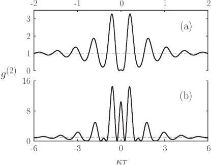
Figure 1: Second-order correlation function for ideal coupling [Eq. (30)]: (a) Parameter Set 1, (b) Parameter Set 2.

In Fig. 1 the magnitude of the antibunching effect—the amplitude of the vacuum Rabi oscillation— is larger than observed in the experiments by approximately an order of magnitude (see Fig. 3). Significant improvement is obtained by taking into account the unequal coupling strengths of atoms randomly distributed throughout the cavity mode.

III.2 Fixed Atomic Configuration

Rempe et al. Rempe et al. (1991) extended the above treatment to the case of unequal coupling strengths, adopting the non-Hermitian Hamiltonian (18) while keeping the number of atoms and the atom locations fixed. For $N$ atoms in a spatial configuration $\{{\bm{r}}_{j}\}$, the second-order correlation function takes the same form as in Eq. (30)—still a perfect square—but with a modified amplitude of oscillation Rempe et al. (1991); Car (e):

$$g^{(2)}_{\{{\bm{r}}_{j}\}}(\tau)=\left\{1-\frac{[1+\xi(1+C_{\{{\bm{r}}_{j}\}})]S_{\{{\bm{r}}_{j}\}}-2C_{\{{\bm{r}}_{j}\}}}{1+(1+\xi/2)S_{\{{\bm{r}}_{j}\}}}\,e^{-\frac{1}{2}(\kappa+\gamma/2)\tau}\!\left[\cos\left(\Omega\tau\right)+\frac{\frac{1}{2}(\kappa+\gamma/2)}{\Omega}\sin\left(\Omega\tau\right)\right]\right\}^{2},$$ (34)

with

$$C_{\{{\bm{r}}_{j}\}}\equiv\sum_{j=1}^{N}C_{1j},\qquad C_{1j}\equiv g^{2}({\bm{r}}_{j})/\kappa\gamma,$$ (35)

$$S_{\{{\bm{r}}_{j}\}}\equiv\sum_{j=1}^{N}\frac{2C_{1j}}{1+\xi(1+C_{\{{\bm{r}}_{j}\}})-2\xi C_{1j}},$$ (36)

where the vacuum Rabi frequency is given by Eq. (31) with effective number of interacting atoms

$$\bar{N}_{\rm eff}\to N^{\{{\bm{r}}_{j}\}}_{\rm eff}\equiv\sum_{j=1}^{N}g^{2}({\bm{r}}_{j})/g_{\rm max}^{2}.$$ (37)

III.3 Monte-Carlo Average and Comparison with Experimental Results

In reality the number of atoms and their configuration both fluctuate in time. These fluctuations are readily taken into account if the typical atomic motion is sufficiently slow; one takes a stationary-atom Monte-Carlo average over configurations, adopting a finite interaction volume $V_{F}$ and combining a Poisson average over the number of atoms $N$ with an average over their uniformly distributed positions ${\bm{r}}_{j}$, $j=1,\ldots,N$. In particular, the effective number of interacting atoms becomes

$$\bar{N}_{\rm eff}=\overline{N^{\{{\bm{r}}_{j}\}}_{\rm eff}},$$ (38)

where the overbar denotes the Monte-Carlo average.

Although it is not justified by the velocities listed in Table 1, a stationary-atom approximation was adopted when modeling the experimental results in Refs. Rempe et al. (1991) and Foster et al. (2000a). The correlation function was computed as the Monte-Carlo average

$$g^{(2)}(\tau)=\overline{g^{(2)}_{\{{\bm{r}}_{j}\}}(\tau)},$$ (39)

with $g^{(2)}_{\{{\bf r}_{j}\}}(\tau)$ given by Eq. (34). In fact, taking a Monte-Carlo average over normalized correlation functions in this way is not, strictly, correct. In practice, first the delayed photon coincidence rate is measured, as a separate average, then subsequently normalized by the average photon counting rate. The more appropriate averaging procedure is therefore

$$g^{(2)}(\tau)=\frac{\overline{\langle\hat{a}^{\dagger}(0)\hat{a}^{\dagger}(\tau)\hat{a}(\tau)\hat{a}(0)\rangle_{\{{\bm{r}}_{j}\}}}}{\left(\overline{\langle\hat{a}^{\dagger}\hat{a}\rangle_{\{{\bm{r}}_{j}\}}}\mkern 2.0mu\right)^{2}},$$ (40)

or, in a form revealing more directly the relationship to Eq. (34), the average is to be weighted by the square of the photon number:

$$g^{(2)}(\tau)=\frac{\overline{\left(\left\langle\hat{a}^{\dagger}\hat{a}\right\rangle_{\{{\bm{r}}_{j}\}}\right)^{2}g^{(2)}_{\{{\bm{r}}_{j}\}}(\tau)}}{\left(\overline{\langle\hat{a}^{\dagger}\hat{a}\rangle_{\{{\bm{r}}_{j}\}}}\mkern 2.0mu\right)^{2}},$$ (41)

where

$$\langle\hat{a}^{\dagger}\hat{a}\rangle_{\{{\bm{r}}_{j}\}}=\left(\frac{{\cal E}/\kappa}{1+2C_{\{{\bm{r}}_{j}\}}}\right)^{2}$$ (42)

is the intracavity photon number expectation—in stationary state $|\psi_{\rm ss}\rangle$ [Eq. (19)]—for the configuration of atoms $\{{\bm{r}}_{j}\}$.

Note that the statistical independence of forwards-scattering events that are widely separated in time yields the limit

$$\lim_{\tau\to\infty}g^{(2)}_{\{{\bm{r}}_{j}\}}(\tau)\to 1,$$ (43)

which clearly holds for the average (39) as well. Equation (41), on the other hand, yields

$$\lim_{\tau\to\infty}g^{(2)}(\tau)\to\overline{\left(\left\langle\hat{a}^{\dagger}\hat{a}\right\rangle_{\{{\bm{r}}_{j}\}}\right)^{2}}\bigg{/}\left(\overline{\langle\hat{a}^{\dagger}\hat{a}\rangle_{\{{\bm{r}}_{j}\}}}\mkern 2.0mu\right)^{2}\geq 1.$$ (44)

A value greater than unity arises because while there are fluctuations in $N$ and $\{{\bm{r}}_{j}\}$, their correlation time is infinite under the stationary-atom approximation; the expected decay of the correlation function to unity is therefore not observed.

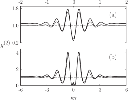
Figure 2: Second-order correlation function with Monte-Carlo average over number of atoms $N$ and configuration $\{{\bm{r}_{j}}\}$. The average is taken according to Eq. (39) (thin line) and Eq. (41) (thick line) for (a) Parameter Set 1, (b) Parameter Set 2.

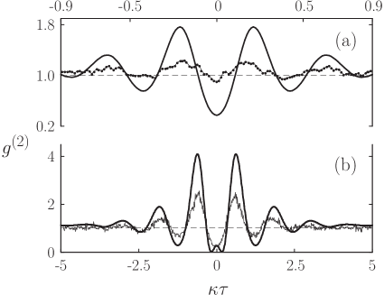
Figure 3: Second-order correlation function with Monte-Carlo average, Eq. (41), over number of atoms $N$ and configuration $\{{\bm{r}_{j}}\}$ compared with the experimental data from (a) Fig. 4(a) of Ref. Rempe et al. (1991) (Parameter Set 1) and (b) Fig. 4 of Ref. Foster et al. (2000a) (Parameter Set 2).

The two averaging schemes are compared in the plots of Fig. 2, which suggest that atomic beam fluctuations should have at least a small effect in the experiments; although, just how important they turn out to be is not captured at all by the figure. The actual disagreement between the model and the data is displayed in Fig. 3. The measured photon antibunching effect is significantly smaller than predicted in both experiments: smaller by a factor of 4 in Fig. 3(a), as the authors of Ref. Rempe et al. (1991) explicitly state, and by a factor of a little more than 2 in Fig. 3(b).

The rest of the paper is devoted to a resolution of this disagreement. It certainly arises from a breakdown of the stationary-atom approximation as suggested by Rempe et al. Rempe et al. (1991). Physics beyond the addition of a finite correlation time for fluctuations of $N(t)$ and $\{{\bm{r}}_{j}(t)\}$ is needed, however. We aim to show that the single most important factor is the alignment of the atomic beam.

IV Delayed Photon Coincidences for an Atomic Beam

We return now to the full atomic beam simulation outlined in Sec. II. With the beam perpendicular to the cavity axis, the rate of change of the dipole coupling constants might be characterized by the cavity-mode transit time, determined from the mean atomic speed and the cavity-mode waist. Taking the values of these quantities from Table 1, the experiment of Rempe et al. has $w_{0}/\bar{v}_{\rm source}=182\mkern 2.0mu{\rm nsec}$, which should be compared with a vacuum-Rabi-oscillation decay time $2(\kappa+\gamma/2)^{-1}=94\mkern 2.0mu{\rm nsec}$, while Foster et al. have $w_{0}/\bar{v}_{\rm source}=66\mkern 2.0mu{\rm nsec}$ and a decay time $2(\kappa+\gamma/2)^{-1}=29\mkern 2.0mu{\rm nsec}$. In both cases, the ratio between the transit time and decay time is $\sim 2$; thus, we might expect the internal state dynamics to follow the atomic beam fluctuations adiabatically, to a good approximation at least, thus providing a justifying for the stationary-atom approximation. Figure 3 suggests that this is not so. Our first task, then, is to see how well in practice the adiabatic following assertion holds.

IV.1 Monte-Carlo Simulation of the Atomic Beam: Effect of Beam Misalignment

Atomic beam fluctuations induce fluctuations of the intracavity photon number expectation, as illustrated by the examples in Figs. 5 and 5. Consider the two curves (a) in these figures first, where the atomic beam is aligned perpendicular to the cavity axis. The ringing at regular intervals along these curves is the transient response to enforced cavity-mode quantum jumps—jumps enforced to sample the quantum fluctuations efficiently (see Sec. IV.2). Ignoring these perturbations for the present, we see that with the atomic beam aligned perpendicular to the cavity axis the fluctuations evolve more slowly than the vacuum Rabi oscillation—at a similar rate, in fact, to the vacuum Rabi oscillation decay. As anticipated, an approximate adiabatic following is plausible.

Consider now the two curves (b); these introduce a $9.6\mkern 2.0mu{\rm mrad}$ misalignment of the atomic beam, following up on the comment of Foster et al. Foster et al. (2000a) that misalignments as large as $1^{\circ}$ ($17.45\mkern 2.0mu{\rm mrad}$) might occur. The changes in the fluctuations are dramatic. First, their size increases, though by less on average than it might appear. The altered distributions of intracavity photon numbers are shown in Fig. 6. The means are not so greatly changed, but the variances (measured relative to the square of the mean) increase by a factor of 2.25 in Fig. 5 and 1.45 in Fig. 5. Notably, the distribution is asymmetric, so the most probable photon number lies below the mean. The asymmetry is accentuated by the tilt, especially for Parameter Set 1 [Fig. 6(a)].

More important than the change in amplitude of the fluctuations, though, is the increase in their frequency. Again, the most significant effect occurs for Parameter Set 1 (Fig. 5), where the frequency with a $9.6\mkern 2.0mu{\rm mrad}$ tilt approaches that of the vacuum Rabi oscillation itself; clearly, there can be no adiabatic following under these conditions. Indeed, the net result of the changes from Fig. 5(a) to Fig. 5(b) is that the quantum fluctuations, initiated in the simulation by quantum jumps, are completely lost in a background of classical noise generated by the atomic beam. It is clear that an atomic beam misalignment of sufficient size will drastically reduce the photon antibunching effect observed.

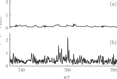
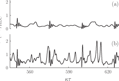
Figure 4: Typical trajectory of the intracavity photon number expectation for Parameter Set 1: (a) atomic beam aligned perpendicular to the cavity axis, (b) with a $9.6\mkern 2.0mu{\rm mrad}$ tilt of the atomic beam. The driving field strength is ${\mathcal{E}}/\kappa=2.5\times 10^{-2}$.

Figure 5: As in Fig. 5 but for Parameter Set 2.

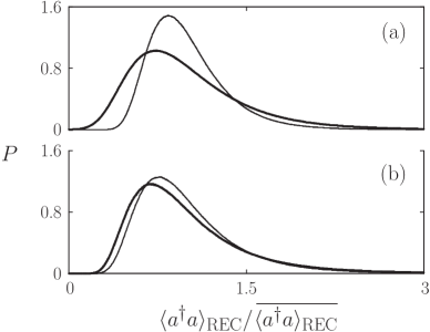
Figure 6: Distribution of intracavity photon number expectation with the atom beam perpendicular to the cavity axis (thin line) and a $9.6\mkern 2.0mu{\rm mrad}$ tilt of the atomic beam (thick line): (a) Parameter Set 1, (b) Parameter Set 2.

For a more quantitative characterization of its effect, we carried out quantum trajectory simulations in a one-quantum truncation (without quantum jumps) and computed the semiclassical photon number correlation function

$$g^{(2)}_{\rm sc}(\tau)=\frac{\overline{\langle(\hat{a}^{\dagger}\hat{a})(t)\rangle_{\rm REC}\langle(\hat{a}^{\dagger}\hat{a})(t+\tau)\rangle_{\rm REC}}}{\left(\overline{\langle(\hat{a}^{\dagger}\hat{a})(t)\rangle_{\rm REC}}\mkern 2.0mu\right)^{2}},$$ (45)

where the overbar denotes a time average (in practice an average over an ensemble of sampling times $t_{k}$). The photon number expectation was calculated in two ways: first, by assuming that the conditional state adiabatically follows the fluctuations of the atomic beam, in which case, from Eq. (42), we may write

$$\langle(\hat{a}^{\dagger}\hat{a})(t)\rangle_{\rm REC}=\left(\frac{{\cal E/\kappa}}{1+2C_{\{{\bm{r}_{j}}(t)\}}}\right)^{2},$$ (46)

and second, without the adiabatic assumption, in which case the photon number expectation was calculated from the state vector in the normal way.

Correlation functions computed for different atomic beam tilts according to this scheme are plotted in Figs. 7 and 8. In each case the curves shown in the left column assume adiabatic following while those in the right column do not. The upper-most curves [frames (a) and (e)] hold for a beam aligned perpendicular to the cavity axis and those below [frames (b)–(d) and (f)–(h)] show the effects of increasing misalignment of the atomic beam.

A number of comments are in order. Consider first the aligned atomic beam. Correlation times read from the figures are in approximate agreement with the cavity-mode transit times computed above: the numbers are $191\mkern 2.0mu{\rm nsec}$ and $167\mkern 2.0mu{\rm nsec}$ from frames (a) and (e), respectively, of Fig. 7, compared with $w_{0}/\bar{v}_{\rm oven}=182\mkern 2.0mu{\rm nsec}$; and $68\mkern 2.0mu{\rm nsec}$ and $53\mkern 2.0mu{\rm nsec}$ from frames (a) and (e) of Fig. 8, respectively, compared with $w_{0}/\bar{v}_{\rm oven}=66\mkern 2.0mu{\rm nsec}$. The numbers show a small decrease in the correlation time when the adiabatic following assumption is lifted (by 10-20%) but no dramatic change; and there is a corresponding small increase in the fluctuation amplitude.

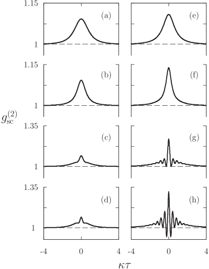
Figure 7: Semiclassical correlation function for Parameter Set 1, with adiabatic following of the photon number (left column) and without adiabatic following (right column); for atomic beam tilts of (a,e) $0\mkern 2.0mu{\rm mrad}$, (b,f) $4\mkern 2.0mu{\rm mrad}$, (c,g) $9\mkern 2.0mu{\rm mrad}$, (d,h) $13\mkern 2.0mu{\rm mrad}$.

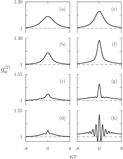
Figure 8: As in Fig. 7 but for Parameter Set 2 and atomic beam tilts of (a,e) $0\mkern 2.0mu{\rm mrad}$, (b,f) $10\mkern 2.0mu{\rm mrad}$, (c,g) $17\mkern 2.0mu{\rm mrad}$, (d,h) $34\mkern 2.0mu{\rm mrad}$.

Consider now the effect of an atomic beam tilt. Here the changes are significant. They are most evident in frames (d) and (h) of each figure, but clear already in frames (c) and (g) of Fig. 7, and frames (b) and (f) of Fig. 8, where the tilts are close to the tilt used to generate Figs. 5(b) and 5(b) (also to those used for the data fits in Sec. IV.2). There is first an increase in the magnitude of the fluctuations—the factors 2.25 and 1.45 noted above—but, more significant, a separation of the decay into two pieces: a central component, with short correlation time, and a much broader component with correlation time larger than $w_{0}/\bar{v}_{\rm oven}$. Thus, for a misaligned atomic beam, the dynamics become notably nonadiabatic.

Our explanation of the nonadiabaticity begins with the observation that any tilt introduces a velocity component along the standing wave, with transit times through a quarter wavelength of $\lambda/4\bar{v}_{\rm oven}\sin\theta=86\mkern 2.0mu{\rm nsec}$ in the Rempe et al. Rempe et al. (1991) experiment and $\lambda/4\bar{v}_{\rm oven}\sin\theta=60\mkern 2.0mu{\rm nsec}$ in the Foster et al. Foster et al. (2000a) experiment. Compared with the transit time $w_{0}/\bar{v}_{\rm oven}$, these numbers have moved closer to the decay times of the vacuum Rabi oscillation—$94\mkern 2.0mu{\rm nsec}$ and $29\mkern 2.0mu{\rm nsec}$, respectively. Note that the distances traveled through the standing wave during the cavity-mode transit, in time $w_{0}/\bar{v}_{\rm oven}$, are $w_{0}\sin\theta=0.53\lambda$ (Parameter Set 1) and $w_{0}\sin\theta=0.28\lambda$ (Parameter Set 2). It is difficult to explain the detailed shape of the correlation function under these conditions. Speaking broadly, though, fast atoms produce the central component, the short correlation time associated with nonadiabatic dynamics, while slow atoms produce the background component with its long correlation time, which follows from an adiabatic response. Increased tilt brings greater separation between the responses to fast and slow atoms.

Simple functional fits to the curves in frame (g) of Fig. 7 and frame (f) of Fig. 8 yield short correlation times of 40-50$\mkern 2.0mu{\rm nsec}$ and $20\mkern 2.0mu{\rm nsec}$, respectively. Consistent numbers are recovered by adding the decay rate of the vacuum Rabi oscillation to the inverse travel time through a quarter wavelength; thus, $(1/94+1/86)^{-1}\mkern 2.0mu{\rm nsec}=45\mkern 2.0mu{\rm nsec}$ and $(1/29+1/60)^{-1}\mkern 2.0mu{\rm nsec}=20\mkern 2.0mu{\rm nsec}$, respectively, in good agreement with the correlation times deduced from the figures.

The last and possibly most important thing to note is the oscillation in frames (g) and (h) of Fig. 7 and frame (h) of Fig. 8. Its frequency is the vacuum Rabi frequency, which shows unambiguously that the oscillation is caused by a nonadiabatic response of the intracavity photon number to the fluctuations of the atomic beam. For the tilt used in frame (g) of Fig. 7, the transit time through a quarter wavelength is approximately equal to the vacuum-Rabi-oscillation decay time, while it is twice that in frame (f) of Fig. 8. As the tilts used are close to those giving the best data fits in Sec. IV.2, this would suggest that atomic beam misalignment places the experiment of Rempe et al. Rempe et al. (1991) further into the nonadiabatic regime than that of Foster et al. Foster et al. (2000a), though the tilt is similar in the two cases. The observation is consistent with the greater contamination by classical noise in Fig. 5(b) than in Fig. 5(b) and with the larger departure of the Rempe et al. data from the stationary-atom model in Fig. 3.

IV.2 Simulation Results and Data Fits

The correlation functions in the right-hand column of Figs. 7 and 8 account for atomic-beam-induced classical fluctuations of the intracavity photon number. While some exhibit a vacuum Rabi oscillation, the signals are, of course, photon bunched; a correlation function like that of Fig. 7(g) provides evidence of collective strong coupling, but not of strong coupling of the one-atom kind, for which a photon antibunching effect is needed. We now carry out full quantum trajectory simulations in a two-quanta truncation to recover the photon antibunching effect—i.e., we bring back the quantum jumps.

In the weak-field limit the normalized photon correlation function is independent of the amplitude of the driving field ${\cal E}$ [Eqs. (30) and (34)]. The forwards photon scattering rate itself is proportional to $({\cal E}/\kappa)^{2}$ [Eq. (42)], and must be set in the simulations to a value very much smaller than the inverse vacuum-Rabi-oscillation decay time [Eq. (22)]. Typical values of the intracavity photon number were $\sim 10^{-7}-10^{-6}$. It is impractical, under these conditions, to wait for the natural occurrence of forwards-scattering quantum jumps. Instead, cavity-mode quantum jumps are enforced at regular sample times $t_{k}$ [see Figs. 5(a) and 5(a)]. Denoting the record with enforced cavity-mode jumps by $\overline{\vbox{\vskip 7.5pt}{\rm REC}\mkern-2.0mu}\mkern 2.0mu$, the second-order correlation function is then computed as the ratio of ensemble averages

$$g^{(2)}(\tau)=\frac{\overline{\langle(\hat{a}^{\dagger}\hat{a})(t_{k})\rangle_{\overline{{\rm REC}\mkern-4.0mu}}\mkern 4.0mu\langle(\hat{a}^{\dagger}\hat{a})(t_{k}+\tau)\rangle_{\overline{{\rm REC}\mkern-4.0mu}}\mkern 4.0mu}}{\left(\overline{\langle(\hat{a}^{\dagger}\hat{a})(t_{l})\rangle_{\overline{{\rm REC}\mkern-4.0mu}}\mkern 4.0mu}\mkern 2.0mu\right)^{\mkern-2.0mu2}}\mkern 2.0mu,$$ (47)

where the sample times in the denominator, $t_{l}$, are chosen to avoid the intervals—of duration a few correlation times—immediately after the jump times $t_{k}$; this ensures that both ensemble averages are taken in the steady state. With the cut-off parameter [Eq. (6)] set to $F=0.01$, the number of atoms within the interaction volume typically fluctuates around $N(t)\sim 400$-$450$ atoms for Parameter Set 1 and $N(t)\sim 280$-$320$ atoms for Parameter Set 2; in a two-quanta truncation, the corresponding numbers of state amplitudes are $\sim 90,000$ (Parameter Set 1) and $\sim 45,000$ (Parameter Set 2).

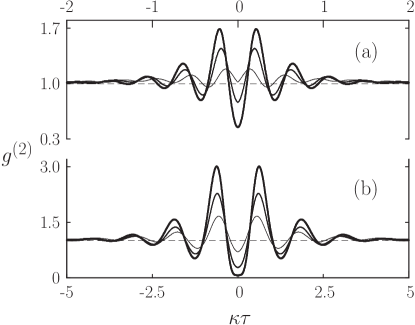
Figure 9: Second-order correlation function from full quantum trajectory simulations with a two-quanta truncation: (a) Parameter Set 1 and $\theta=0\mkern 2.0mu{\rm mrad}$ (thick line), $7\mkern 2.0mu{\rm mrad}$ (medium line), $12\mkern 2.0mu{\rm mrad}$ (thin line); (b) Parameter Set 2 and $\theta=0\mkern 2.0mu{\rm mrad}$ (thick line), $10\mkern 2.0mu{\rm mrad}$ (medium line), $17\mkern 2.0mu{\rm mrad}$ (thin line).

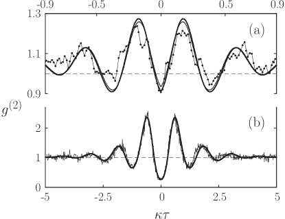
Figure 10: Best fits to experimental results: (a) data from Fig. 4(a) of Ref. Rempe et al. (1991) are fitted with Parameter Set 1 and $\theta=9.7\mkern 2.0mu{\rm mrad}$ (thick line) and $10\mkern 2.0mu{\rm mrad}$ (thin line); (b) data from Fig. 4 of Ref. Foster et al. (2000a) are fitted with Parameter Set 2 and $\theta=9.55\mkern 2.0mu{\rm mrad}$. Averages of (a) 200,000 and (b) 50,000 samples were taken with a cavity-mode cut-off $F=0.01$.

Figure 9 shows the computed correlation functions for various atomic beam tilts. We select from a series of such results the one that fits the measured correlation function most closely. Optimum tilts are found to be $9.7\mkern 2.0mu{\rm mrad}$ for the Rempe et al. Rempe et al. (1991) experiment and $9.55\mkern 2.0mu{\rm mrad}$ for the experiment of Foster et al. Foster et al. (2000a). The best fits are displayed in Fig. 10. In the case of the Foster et al. data the fit is extremely good. The only obvious disagreement is that the fitted frequency of the vacuum Rabi oscillation is possibly a little low. This could be corrected by a small increase in atomic beam density—the parameter $\bar{N}_{\rm eff}$—which is only known approximately from the experiment, in fact by fitting the formula (31) to the data.

The fit to the data of Rempe et al. Rempe et al. (1991) is not quite so good, but still convincing with some qualifications. Note, in particular, that the tilt used for the fit might be judged a little too large, since the three central minima in Fig. 10(a) are almost flat, while the data suggest they should more closely follow the curve of a damped oscillation. As the thin line in the figure shows, increasing the tilt raises the central minimum relative to the two on the side; thus, although a better fit around $\kappa\tau=0$ is obtained, the overall fit becomes worse. This trend results from the sharp maximum in the semiclassical correlation function of Fig. 7(g), which becomes more and more prominent as the atomic beam tilt is increased.

The fit of Fig. 10(b) is extremely good, and, although it is not perfect, the thick line in Fig. 10(a), with a $9.7\mkern 2.0mu{\rm mrad}$ tilt, agrees moderately well with the data once the uncertainty set by shot noise is included, i.e., adding error bars of a few percent (see Fig. 13). Thus, leaving aside possible adjustments due to omitted noise sources, such as spontaneous emission—to which we return in Sec. V—and atomic and cavity detunings, the results of this and the last section provide strong support for the proposal that the disagreement between theory and experiment presented in Fig. 3 arises from an atomic beam misalignment of approximately $0.5^{\circ}$.

One final observation should be made regarding the fit to the Rempe et al. Rempe et al. (1991) data. Figure 11 replots the comparison made in Fig. 10(a) for a larger range of time delays. Frame (a) plots the result of our simulation for a perfectly aligned atomic beam, and frames (b) and (c) shows the results, plotted in Fig. 10(a), corresponding to atomic beam tilts of $\theta=9.7\mkern 2.0mu{\rm mrad}$ and $10\mkern 2.0mu{\rm mrad}$, respectively. The latter two plots are overlayed by the experimental data. Aside from the reduced amplitude of the vacuum Rabi oscillation, in the presence of the tilt the correlation function exhibits a broad background arising from atomic beam fluctuations. Notably, the background is entirely absent when the atomic beam is aligned. The experimental data exhibit just such a background (Fig. 3(a) of Ref. Rempe et al. (1991)); moreover, an estimate, from Fig. 11, of the background correlation time yields approximately $400\mkern 2.0mu{\rm nsec}$, consistent with the experimental measurement. It is significant that this number is more than twice the transit time, $w_{0}/\bar{v}_{\rm oven}=182\mkern 2.0mu{\rm nsec}$, and therefore not explained by a perpendicular transit across the cavity mode. In fact the background mimics the feature noted for larger tilts in Figs. 7 and 8; as mentioned there, it appears to find its origin in the separation of an adiabatic (slowest atoms) from a nonadiabatic (fastest atoms) response to the density fluctuations of the atomic beam.

Note, however, that a correlation time of $400\mkern 2.0mu{\rm nsec}$ appears to be consistent with a perpendicular transit across the cavity when the cavity-mode transit time is defined as $2w_{0}/\bar{v}_{\rm oven}=364\mkern 2.0mu{\rm nsec}$, or, using the peak rather than average velocity, as $4w_{0}/\sqrt{\pi}\bar{v}_{\rm oven}=411\mkern 2.0mu{\rm nsec}$; the latter definition was used to arrive at the $400\mkern 2.0mu{\rm nsec}$ quoted in Ref. Rempe et al. (1991). There is, of course, some ambiguity in how a transit time should be defined. We are assuming that the time to replace an ensemble of interacting atoms with a statistically independent one—which ultimately is what determines the correlation time—is closer to $w_{0}/\bar{v}_{\rm oven}$ than $2w_{0}/\bar{v}_{\rm oven}$. In support of the assumption we recall that the number obtained in this way agrees with the semiclassical correlation function for an aligned atomic beam [Figs. 7 and 8, frame (a)].

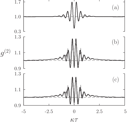
Figure 11: Second-order correlation function from full quantum trajectory simulations with a two-quanta basis for Parameter Set 1 and (a) $\theta=0\mkern 2.0mu{\rm mrad}$, (b) $\theta=9.7\mkern 2.0mu{\rm mrad}$, (c) $\theta=10\mkern 2.0mu{\rm mrad}$. Averages of (a) 15,000, and (b) and (c) 200,000 samples were taken with a cavity-mode cut-off $F=0.01$.

IV.3 Mean-Doppler-Shift Compensation

Foster et al. Foster et al. (2000a), in an attempt to account for the disagreement of their measurements and the stationary-atom model, extended the results of Sec. III.2 to include an atomic detuning. They then fitted the data using the following procedure: (i) the component of atomic velocity along the cavity axis is viewed as a Doppler shift from the stationary-atom resonance, (ii) the mean shift is assumed to be offset by an adjustment of the driving field frequency (tuning to moving atoms) at the time the data are taken, and (iii) an average over residual detunings—deviations from the mean—is taken in the model, i.e., the detuning-dependent generalization of Eq. (34). The approach yields a reasonable fit to the data (Fig. 6 of Ref. Foster et al. (2000a)).

The principal difficulty with this approach is that a standing-wave cavity presents an atom with two Doppler shifts, not one. It seems unlikely, then, that adjusting the driving field frequency to offset one shift and not the other could compensate for even the average effect of the atomic beam tilt. This difficulty is absent in a ring cavity, though, so we first assess the performance of the outlined prescription in the ring-cavity case.

In a ring cavity, the spatial dependence of the coupling constant [Eq. (11)] is replaced by

$$g({\bm{r}}_{j}(t))=\frac{g_{\rm max}}{\sqrt{2}}\exp(ikz_{j}(t))\exp\!\left[-\frac{x_{j}^{2}(t)+y_{j}^{2}(t)}{w_{0}^{2}}\right],$$ (48)

where the factor $\sqrt{2}$ ensures that the collective coupling strength and vacuum Rabi frequency remain the same. Figure 12(a) shows the result of a numerical implementation of the proposed mean-Doppler-shift compensation for an atomic beam tilt of $17.3\mkern 2.0mu{\rm mrad}$, as used in Fig. 6 of Ref.  Foster et al. (2000a). It works rather well. The compensated curve (thick line) almost recovers the full photon antibunching effect that would be seen with an aligned atomic beam (thin line). The degradation that remains is due to the uncompensated dispersion of velocities (Doppler shifts) in the atomic beam.

For the case of a standing-wave cavity, on the other hand, the outcome is entirely different. This is shown by Fig. 12(b). There, offsetting one of the two Doppler shifts only makes the degradation of the photon antibunching effect worse. In fact, we find that any significant detuning of the driving field from the stationary atom resonance is highly detrimental to the photon antibunching effect and inconsistent with the Foster et al. data.

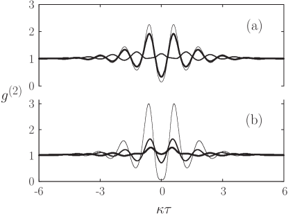
Figure 12: Doppler-shift compensation for a misaligned atomic beam in (a) ring and (b) standing-wave cavities (Parameter Set 2). The second-order correlation function is computed with the atomic beam perpendicular to the cavity axis (thin line), a $17.3\mkern 2.0mu{\rm mrad}$ tilt of the atomic beam (medium line), and a $17.3\mkern 2.0mu{\rm mrad}$ tilt plus compensating detuning of the cavity and stationary atom resonances $\Delta\omega/\kappa=k\bar{v}_{\rm oven}\sin\theta/\kappa=0.916$ (thick line).

V Intracavity Photon Number

The best fits displayed in Fig. 10 were obtained from simulations with a two-quanta truncation and premised upon the measurements being made in the weak-field limit. The strict requirement of the limit sets a severe constraint on the intracavity photon number. We consider now whether the requirement is met in the experiments.

Working from Eqs. (23a) and (23b), and the solution to Eq. (19), a fixed configuration $\{{\bm{r}}_{j}\}$ of $N$ atoms (Sec. III.2) yields photon scattering rates Carmichael et al. (1991); Brecha et al. (1999); Car (c)

$$R_{\rm forwards}=2\kappa\langle\hat{a}^{\dagger}\hat{a}\rangle_{\rm REC}=2\kappa\mkern-3.0mu\left(\frac{{\cal E/\kappa}}{1+2C_{\{{\bm{r}_{j}}\}}}\right)^{\mkern-2.0mu2},$$ (49a)

and

$$R_{\rm side} = \gamma\sum_{k=1}^{N}\langle\hat{\sigma}_{k+}\hat{\sigma}_{k-}\rangle$$ (49b)

$$= \gamma\sum_{k=1}^{N}\left(\frac{g({\bm{r}}_{k})}{\gamma/2}\frac{{\cal E/\kappa}}{1+2C_{\{{\bm{r}_{j}}\}}}\right)^{\mkern-2.0mu2}$$

$$= 2C_{\{{\bm{r}}_{j}\}}2\kappa\langle\hat{a}^{\dagger}\hat{a}\rangle_{\rm REC},$$

with ratio

$$\frac{R_{\rm side}}{R_{\rm forwards}}=2C_{\{{\bm{r}}_{j}\}}=\frac{2N_{\rm eff}^{\{{\bm{r}}_{j}\}}g_{\rm max}^{2}}{\kappa\gamma}\sim\frac{2\bar{N}_{\rm eff}g_{\rm max}^{2}}{\kappa\gamma}.$$ (50)

The weak-field limit [Eq. (22)] requires that the greater of the two rates be much smaller than $\frac{1}{2}(\kappa+\gamma/2)$; it is not necessarily sufficient that the forwards scattering rate be low. The side scattering (spontaneous emission) rate is larger than the forwards scattering rate in both of the experiments being considered—larger by a large factor of $70$–$80$. Thus, from Eqs. (49a) and (50), the constraint on intracavity photon number may be written as

$$\langle\hat{a}^{\dagger}\hat{a}\rangle\ll\frac{1+\gamma/2\kappa}{8\bar{N}_{\rm eff}g^{2}_{\rm max}/\kappa\gamma},$$ (51)

where, from Table 1, the right-hand side evaluates as $1.2\times 10^{-2}$ for Parameter Set 1 and $4.7\times 10^{-3}$ for Parameter Set 2, while the intracavity photon numbers inferred from the experimental count rates are $3.8\times 10^{-2}$ Rempe et al. (1991) and $7.6\times 10^{-3}$ Foster et al. (2000a). It seems that neither experiment satisfies condition (51). As an important final step we should therefore relax the weak-driving-field assumption (photon number $\sim 10^{-7}$–$10^{-6}$ in the simulations) and assess what effect this has on the data fits; can the simulations fit the inferred intracavity photon numbers as well?

To address this question we extended our simulations to a three-quanta truncation of the Hilbert space with cavity-mode cut-off changed from $F=0.01$ to $F=0.1$. With the changed cut-off the typical number of atoms in the interaction volume is halved: $N(t)\sim 180$–$220$ atoms for Parameter Set 1 and $N(t)\sim 150$–$170$ atoms for Parameter Set 2, from which the numbers of state amplitudes (including three-quanta states) increase to $1,300,000$ and $700,000$, respectively. The new cut-off introduces a small error in $\bar{N}_{\rm eff}$, hence in the vacuum Rabi frequency, but the error is no larger than one or two percent.

At this point an additional approximation must be made. At the excitation levels of the experiments, even a three-quanta truncation is not entirely adequate. Clumps of three or more side-scattering quantum jumps can occur, and these are inaccurately described in a three-quanta basis. In an attempt to minimize the error, we artificially restrict (through a veto) the number of quantum jumps permitted within some prescribed interval of time. The accepted number was set at two and the time interval to $1\kappa^{-1}$ for Parameter Set 1 and $3\kappa^{-1}$ for Parameter Set 2 (the correlation time measured in cavity lifetimes is longer for Parameter Set 2). With these settings approximately 10% of the side-scattering jumps were neglected at the highest excitation levels considered.

The results of our three-quanta simulations appear in Fig. 13; they use the optimal atomic beam tilts of Fig. 10. Figure 13(a) compares the simulation with the data of Rempe et al. Rempe et al. (1991) at an intracavity photon number that is approximately six times smaller than what we estimate for the experiment (a more realistic simulation requires a higher level of truncation and is impossible for us to handle numerically). The overall fit in Fig. 13 is as good as that in Fig. 10, with a slight improvement in the relative depths of the three central minima. A small systematic disagreement does remain, however. We suspect that the atomic beam tilt used is actually a little large, while the contribution to the decoherence of the vacuum Rabi oscillation from spontaneous emission should be somewhat more. We are satisfied, nevertheless, that the data of Rempe et al. Rempe et al. (1991) are adequately explained by our model.

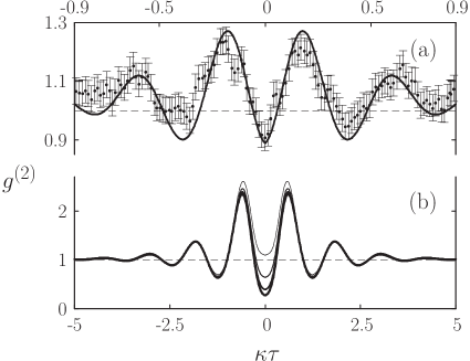
Figure 13: Second-order correlation function from full quantum trajectory simulations with a three-quanta truncation and atomic beam tilts as in Fig. 10: (a) Parameter Set 1, mean intracavity photon number $\langle a^{{\dagger}}a\rangle=6.7\times 10^{-3}$; (b) Parameter Set 2, mean intracavity photon numbers $\langle a^{{\dagger}}a\rangle=2.2\times 10^{-4}$, $5.7\times 10^{-4}$, $1.1\times 10^{-3}$, and $1.7\times 10^{-3}$ (thickest curve to thinest curve). Averages of 20,000 samples were taken with a cavity-mode cut-off $F=0.1$. Shot noise error bars are added to the data taken from Ref. Rempe et al. (1991).

Results for the experiment of Foster et al Foster et al. (2000a) lead in a rather different direction. They are displayed in Fig. 13(b), where four different intracavity photon numbers are considered. The lowest, $\langle\hat{a}^{\dagger}\hat{a}\rangle=2.2\times 10^{-4}$, reproduces the weak-field result of Fig. 10(b). As the photon number is increased, the fit becomes progressively worse. Even at the very low value of $5.7\times 10^{-4}$ intracavity photons, spontaneous emission raises the correlation function for zero delay by a noticeable amount. Then we obtain $g^{(2)}(0)>1$ at the largest photon number considered. Somewhat surprisingly, even this photon number, $\langle\hat{a}^{\dagger}\hat{a}\rangle=1.7\times 10^{-3}$, is smaller than that estimated for the experiment—smaller by a factor of five. Our simulations therefore disagree significantly with the measurements, despite the near perfect fit of Fig. 10(b). The simplest resolution would be for the estimated photon number to be too high. A reduction by more than an order of magnitude is needed, however, implying an unlikely error, considering the relatively straightforward method of inference from photon counting rates. This anomaly, for the present, remains unresolved.

VI Conclusions

Spatial variation of the dipole coupling strength has for many years been a particular difficulty for cavity QED at optical frequencies. The small spatial scale set by the optical wavelength makes any approach to a resolution a formidable challenge. There has nevertheless been progress made with cooled and trapped atoms Hood et al. (2000); Pinkse et al. (2000); Boca et al. (2004); Maunz et al. (2005); Birnbaum et al. (2005); Hennrich et al. (2005), and in semiconductor systems Yoshie et al. (2004); Reithmaier et al. (2004); Peter et al. (2005) where the participating ‘atoms’ are fixed.

The earliest demonstrations of strong coupling at optical frequencies employed standing-wave cavities and thermal atomic beams, where control over spatial degrees of freedom is limited to the alignment of the atomic beam. Of particular note are the measurements of photon antibunching in forwards scattering Rempe et al. (1991); Mielke et al. (1998); Foster et al. (2000a). They provide a definitive demonstration of strong coupling at the one-atom level; although many atoms might couple to the cavity mode at any time, a significant photon antibunching effect occurs only when individual atoms are strongly coupled.

Spatial effects pose difficulties of a theoretical nature as well. Models that ignore them can point the direction for experiments, but fail, ultimately, to account for experimental results. In this paper we have addressed a long-standing disagreement of this kind—disagreement between the theory of photon antibunching in forwards scattering for stationary atoms in a cavity Carmichael (1985); Rice and Carmichael (1988); Carmichael et al. (1991); Brecha et al. (1999); Rempe et al. (1991) and the aforementioned experiments Rempe et al. (1991); Mielke et al. (1998); Foster et al. (2000a). Ab initio quantum trajectory simulations of the experiments have been carried out, including a Monte-Carlo simulation of the atomic beam. Importantly, we allow for a misalignment of the atomic beam, since this was recognized as a critical issue in Ref. Foster et al. (2000a). We conclude that atomic beam misalignment is, indeed, the most likely reason for the degradation of the measured photon antibunching effect from predicted results. Working first with a two-quanta truncation, suitable for the weak-field limit, data sets measured by Rempe et al. Rempe et al. (1991) and Foster et al. Foster et al. (2000a) were fitted best by atomic beam tilts from perpendicular to the cavity axis of $9.7\mkern 2.0mu{\rm mrad}$ and $9.55\mkern 2.0mu{\rm mrad}$, respectively.

Atomic motion is recognized as a source of decorrelation omitted from the model used to fit the measurements in Ref. Rempe et al. (1991). We found that the mechanism is more complex than suggested there, however. An atomic beam tilt of sufficient size results in a nonadiabatic response of the intracavity photon number to the inevitable density fluctuations of the beam. Thus classical noise is written onto the forwards-scattered photon flux, obscuring the antibunched quantum fluctuations. The parameters of Ref. Rempe et al. (1991) are particularly unfortunate in this regard, since the nonadiabatic response excites a bunched vacuum Rabi oscillation, which all but cancels out the antibunched oscillation one aims to measure.

Although both of the experiments modeled operate at relatively low forwards scattering rates, neither is strictly in the weak-field limit. We have therefore extended our simulations—subject to some numerical constraints—to assess the effects of spontaneous emission. The fit to the Rempe et al. data Rempe et al. (1991) was slightly improved. We noted that the optimum fit might plausibly be obtained by adopting a marginally smaller atomic beam tilt and allowing for greater decorrelation from spontaneous emission, though a more efficient numerical method would be required to verify this possibility. The fit to the Foster et al. data Foster et al. (2000a) was highly sensitive to spontaneous emission. Even for an intracavity photon number five times smaller than the estimate for the experiment, a large disagreement with the measurement appeared. No explanation of the anomaly has been found.

We have shown that cavity QED experiments can call for elaborate and numerically intensive modeling before a full understanding, at the quantitative level, is reached. Using quantum trajectory methods, we have significantly increased the scope for realistic modeling of cavity QED with atomic beams. While we have shown that atomic beam misalignment has significantly degraded the measurements in an important set of experiments in the field, this observation leads equally to a positive conclusion: potentially, nonclassical photon correlations in cavity QED can be observed at a level at least ten times higher than so far achieved.

References

- Berman (1994) P. R. Berman, ed., Cavity Quantum Electrodynamics, Advances in Atomic, Molecular, and Optical Physics, Supplement 2 (Academic Press, San Diego, 1994).
- Raimond et al. (2001) J. M. Raimond, M. Brune, and S. Haroche, Rev. Mod. Phys. 73, 565 (2001).
- Mabuchi and Doherty (2002) H. Mabuchi and A. Doherty, Nature 298, 1372 (2002).
- Vahala (2003) K. J. Vahala, Nature 424, 839 (2003).
- Khitrova et al. (2006) G. Khitrova, H. M. Gibbs, M. Kira, S. W. Koch, and A. Scherer, Nature Physics 2, 81 (2006).
- Carmichael (2007) H. J. Carmichael, Statistical Methods in Quantum Optics 2: Nonclassical Fields (Springer, Berlin, 2007), pp. 561–766.
- Sanchez-Mondragon et al. (1983) J. J. Sanchez-Mondragon, N. B. Narozhny, and J. H. Eberly, Phys. Rev. Lett. 51, 550 (1983).
- Agarwal (1984) G. S. Agarwal, Phys. Rev. Lett. 53, 1732 (1984).
- Brune et al. (1996) M. Brune, F. Schmidt-Kaler, A. Maali, J. Dreyer, E. Hagley, J. M. Raimond, and S. Haroche, Phys. Rev. Lett. 76, 18003 (1996).
- Bernardot et al. (1992) F. Bernardot, P. Nussenzveig, M. Brune, J. M. Raimond, and S. Haroche, Europhys. Lett. 17, 33 (1992).
- Thompson et al. (1992) R. J. Thompson, G. Rempe, and H. J. Kimble, Phys. Rev. Lett. 68, 1132 (1992).
- Childs et al. (1996) J. J. Childs, K. An, M. S. Otteson, R. R. Dasari, and M. S. Feld, Phys. Rev. Lett. 77, 29013 (1996).
- Boca et al. (2004) A. Boca, R. Miller, K. M. Birnbaum, A. D. Boozer, J. McKeever, and H. J. Kimble, Phys. Rev. Lett. 93, 233603 (2004).
- Maunz et al. (2005) P. Maunz, T. Puppe, I. Schuster, N. Syassen, P. W. H. Pinkse, and G. Rempe, Phys. Rev. Lett. 94, 033002 (2005).
- Yoshie et al. (2004) T. Yoshie, A. Scherer, J. Hendrickson, G. Khitrova, H. M. Gibbs, G. Rupper, C. Ell, O. B. Shchekin, and D. G. Deppe, Nature 432, 200 (2004).
- Reithmaier et al. (2004) J. P. Reithmaier, G. Sek, A. Löffler, C. Hofmann, S. Kuhn, S. Reitzenstein, L. V. Keldysh, V. D. Kulakovskii, T. L. Reinecke, and A. Forchel, Nature 432, 197 (2004).
- Peter et al. (2005) E. Peter, P. Senellart, D. Martrou, A. Lemaître, J. Hours, J. M. Gérard, and J. Bloch, Phys. Rev. Lett. 95, 067401 (2005).
- Wallraff et al. (2004) A. Wallraff, D. I. Schuster, A. Blais, L. Frunzio, R.-S. Huang, J. Majer, S. Kumar, S. M. Girvin, and R. J. Schoelkopf, Nature 431, 162 (2004).
- Car (a) See, for example, H. J. Carmichael, L. Tian, W. Ren, and P. Alsing, “Nonperturbative interactions of photons and atoms in a cavity,” in Ref. Berman (1994), Sect. IIA.
- Raizen et al. (1989) M. G. Raizen, R. J. Thompson, R. J. Brecha, H. J. Kimble, and H. J. Carmichael, Phys. Rev. Lett. 63, 240 (1989).
- Zhu et al. (1990) Y. Z. Zhu, D. J. Gauthier, S. E. Morin, Q. Wu, H. J. Carmichael, and H. J. Kimble, Phys. Rev. Lett. 64, 2499 (1990).
- Gripp et al. (1996) J. Gripp, S. L. Mielke, L. A. Orozco, and H. J. Carmichael, Phys. Rev. A 54, R3746 (1996).
- Weisbuch et al. (1992) C. Weisbuch, M. Nishioka, A. Ishikawa, and Y. Arakawa, Phys. Rev. Lett. 69, 3314 (1992).
- Khitrova et al. (1999) G. Khitrova, H. M. Gibbs, F. Jhanke, M. Kira, and S. W. Koch, Rev. Mod. Phys. 71, 1591 (1999).
- Carmichael (1985) H. J. Carmichael, Phys. Rev. Lett. 55, 2790 (1985).
- Rice and Carmichael (1988) P. R. Rice and H. J. Carmichael, IEEE J. Quantum Electron. 24, 1351 (1988).
- Carmichael et al. (1991) H. J. Carmichael, R. Brecha, and P. R. Rice, Opt. Comm. 82, 73 (1991).
- Brecha et al. (1999) R. J. Brecha, P. R. Rice, and M. Xiao, Phys. Rev. A 59, 2392 (1999).
- Rempe et al. (1991) G. Rempe, R. J. Thompson, R. J. Brecha, W. D. Lee, and H. J. Kimble, Phys. Rev. Lett. 67, 1727 (1991).
- Mielke et al. (1998) S. L. Mielke, G. T. Foster, and L. A. Orozco, Phys. Rev. Lett. 80, 3948 (1998).
- Foster et al. (2000a) G. T. Foster, S. L. Mielke, and L. A. Orozco, Phys. Rev. A 61, 053821 (2000a).
- Birnbaum et al. (2005) K. M. Birnbaum, A. Boca, R. Miller, A. D. Boozer, T. E. Northup, and H. J. Kimble, Nature 436, 87 (2005).
- Imamoḡlu et al. (1979) A. Imamoḡlu, H. Schmidt, G. Woods, and M. Deutsch, Phys. Rev. Lett. 79, 1467 (1979).
- Werner and Imamoḡlu (1999) M. J. Werner and A. Imamoḡlu, Phys. Rev. A 61, 011801 (1999).
- Rebić et al. (1999) S. Rebić, S. M. Tan, A. S. Parkins, and D. F. Walls, J. Opt. B 1, 1464 (1999).
- Rebić et al. (2002) S. Rebić, A. S. Parkins, and S. M. Tan, Phys. Rev. A 65, 063804 (2002).
- Kim et al. (1999) J. Kim, O. Benson, H. Kan, and Y. Yamamoto, Nature 397, 500 (1999).
- Smolyaninov et al. (2002) I. I. Smolyaninov, A. V. Zayats, A. Gungor, and C. C. Davis, Phys. Rev. Lett. 88, 187402 (2002).
- Tian and Carmichael (1992) L. Tian and H. J. Carmichael, Phys. Rev. A 46, R6801 (1992).
- Carmichael and Sanders (1999) H. J. Carmichael and B. C. Sanders, Phys. Rev. A 60, 2497 (1999).
- Martini and Schenzle (2001) U. Martini and A. Schenzle, in Directions in Quantum Optics, edited by H. J. Carmichael, R. J. Glauber, and M. O. Scully (Springer, Berlin, 2001), Lecture Notes in Physics, pp. 238–249.
- Carmichael (1993) H. J. Carmichael, An Open Systems Approach to Quantum Optics (Springer, Berlin, 1993), vol. m18 of Lecture Notes in Physics, pp. 113–179.
- Dalibard et al. (1992) J. Dalibard, Y. Castin, and K. Mølmer, Phys. Rev. Lett. 68, 127902 (1992).
- Dum et al. (1992) L.-M. Dum, P. J. Zoller, and H. Ritsch, Phys. Rev. A 45, 4879 (1992).
- Gardiner and Zoller (2004) C. W. Gardiner and P. Zoller, Quantum Noise (Springer, Berlin, 2004), pp. 341–396, 3rd ed.
- Car (b) Ref. Carmichael (2007), pp. 767-879.
- Brecha (1990) R. J. Brecha, Phd thesis, University of Texas at Austin (1990).
- Foster (1999) G. T. Foster, Phd thesis, State University of New York at Stony Brook (1999).
- Ramsey (1956) N. F. Ramsey, Molecular Beams (Oxford University Press, Oxford, 1956), pp. 11–25.
- Carmichael et al. (1996) H. J. Carmichael, P. Kochan, and B. C. Sanders, Phys. Rev. Lett. 77, 631 (1996).
- Sanders et al. (1997) B. C. Sanders, H. J. Carmichael, and B. F. Wielinga, Phys. Rev. A 55, 1358 (1997).
- (52) For both experiments the cavity mode function is almost plane; the Rayleigh length exceeds the cavity length by a factor of nine in the Rempe et al. experiment Rempe et al. (1991) and by approximately half that amount in the experiment of Foster et al. Foster et al. (2000a).
- Car (c) Ref. Carmichael (2007), pp. 702-710.
- Car (d) Ref. Carmichael (2007), pp. 711-715.
- Carmichael et al. (2000) H. J. Carmichael, H. M. Castro-Beltran, G. T. Foster, and L. A. Orozco, Phys. Rev. Lett. 85, 1855 (2000).
- Foster et al. (2000b) G. T. Foster, L. A. Orozco, H. M. Castro-Beltran, and H. J. Carmichael, Phys. Rev. Lett. 85, 3149 (2000b).
- Foster et al. (2002) G. T. Foster, W. P. Smith, J. E. Reiner, and L. A. Orozco, Phys. Rev. A 66, 033807 (2002).
- Car (e) Ref. Carmichael (2007), pp. 726-733.
- Hood et al. (2000) C. J. Hood, T. W. Lynn, A. C. Doherty, A. S. Parkins, and H. J. Kimble, Science 287, 1447 (2000).
- Pinkse et al. (2000) P. W. H. Pinkse, T. Fischer, P. Maunz, and G. Rempe, Nature 404, 365 (2000).
- Hennrich et al. (2005) M. Hennrich, A. Kuhn, and G. Rempe, Phys. Rev. Lett. 94, 053604 (2005).