Two center multipole expansion method: application to macromolecular systems

Abstract

We propose a new theoretical method for the calculation of the interaction energy between macromolecular systems at large distances. The method provides a linear scaling of the computing time with the system size and is considered as an alternative to the well known fast multipole method. Its efficiency, accuracy and applicability to macromolecular systems is analyzed and discussed in detail.

I Introduction

In recent years, there has been much progress in simulating the structure and dynamics of large molecules at the atomic level, which may include up to thousands and millions of atoms Schulten06 ; Schulten06_1 ; Schulten06_2 ; Meyer03 . For example, amorphous polymers may have segments each with 10000 atoms Meyer03 which associate to form partially crystalline lamellae, random coil regions, and interfaces between these regions, each of which may contribute with special mechanical and chemical properties to the system.

With increasing computer powers nowadays it became possible to study molecular systems of enormous sizes which were not imaginable just several years ago. For example in Schulten06 a molecular dynamics simulations of the complete satellite tobacco mosaic virus was performed which includes up to 1 million of atoms. In that paper the stability of the whole virion and of the RNA core alone were demonstrated, and a pronounced instability was shown for the capsid without the RNA.

The study of structure and dynamics of macromolecules often implies the calculation of the potential energy surface for the system. The potential energy surface of a macromolecule carries a lot of useful information about the system. For example from the potential energy landscape it is possible to estimate the characteristic times for the conformational changes YSSG06_EPJD ; SYSG06_PRE ; SYSG06_JETP and for fragmentation SYSG06_JETP_frag . The potential energy surface of a macromolecular system can be used for studying the thermodynamical processes in the system such as phase transitions SYSG06_JETP_ph_trans . In proteins, the potential energy surface is related to one of the most intriguing problems of protein physics: protein folding SYSG06_JETP_ph_trans ; Chen05 ; Duan98 ; Liwo05 ; Ding02 . The rate constants for complex biochemical reactions can also be established from the analysis of the potential energy surface ElsaPoster ; ElsaPaper .

The calculation of the potential energy surface and molecular dynamics simulations often implies the evaluation of pairwise interactions. The direct method for evaluating these potentials is proportional to $\sim N^{2}$, where $N$ is the number of particles in the system. This places a severe restraint on the treatable size of the system. During the last two decades many different methods have been suggested which provide a linear dependence of the computational cost with respect to $N$ Gunsteren90 ; Petersen94 ; Ding92 ; White94 ; Schmidt91 ; Greengard85 . The most widely used algorithm of this kind is the fast multipole method (FMM) Greengard85 ; Petersen94 ; Ding92 ; White94 ; Schmidt91 ; Boar2000 ; Pincus77 ; Gibbon02 . The critical size of the system at which this method becomes computationally faster than the exact method is accuracy dependent and is very sensitive to the slope in the $N$ dependence of the computational cost. In refs. Schmidt91 ; Ding92 ; Schulten92 critical sizes ranging from $N\approx 300$ to $N\approx 30000$ have been reported. Many discrepancies of the estimates in the critical size arise from differences in the effort of optimizing the algorithm and the underlying code. However, it is also important to optimize the methods themselves with respect to the required accuracy.

The FMM is based on the systematic organization of multipole representations of a local charge distribution, so that each particle interacts with local expansions of the potential. Originally FMM was introduced in Greengard85 by Greengard and Rokhlin. Later, Greengard’s method has been implemented in various forms. Schmidt and Lee Schmidt91 have produced a version based upon the spherical multipoles for both periodic and nonperiodic systems. Zhou and Johnson have implemented the FMM for use on parallel computers Zhao91 , while Board et al have reported both serial and parallel versions of the FMM Schulten92 .

Ding et al introduced a version of the FMM that relies upon Cartesian rather than spherical multipoles Ding92 , which they applied to very large scale molecular dynamics calculations. Additionally they modified Greengard’s definition of the nearest neighbors to increase the proportion of interactions evaluated via local expansions. Shimada et al also developed a cartesian based FMM program Shimada94 , primarily to treat periodic systems described by molecular mechanics potentials. In both cases only low order multipoles were employed, since high accuracy was not sought.

In the present paper we suggest a new method for calculating the interaction energy between macromolecules. Our method also provides a linear scaling of the computational costs with the size of the system and is based on the multipole expansion of the potential. However, the underlying ideas are quite different from the FMM.

Assuming that atoms from different macromolecules interact via a pairwise Coulomb potential, we expand the potential around the centers of the molecules and build a two center multipole expansion using bipolar harmonics algebra. Finally, we obtain a general expression which can be used for calculating the energy and forces between the fragments. This approach is different from the one used in the FMM, where the so-called translational operators were used to expand the potential around a shifted center. Note that the final expression, which we suggest in our theory was not discussed before within the FMM. Similar expressions were discussed since the earlier 50’s (see e.g. Buehler51 ; Joslin84 ; Gupta81 ; Wolf68 ). In these papers the two center multipole expansion was considered as a new form of Coulomb potential expansion, but the expansion was never applied to the study of macromolecular systems.

We consider the interaction of macromolecules via Coulomb potential since this is the only long-range interaction in macromolecules, which is important for the description of the potential energy surface at large distances. Other interaction terms in macromolecular systems are of the short-range type and become important when macromolecules get close to each other SYSG06_JETP_frag . At large distances these terms can be neglected.

In the present paper we show that the method based on the two center multipole expansion can be used for computing the interaction energy between complex macromolecular systems. In section II we present the formalism which lies behind the two center multipole expansion method. In subsection III.1 we analyze the behavior of the computation cost of this method and establish the critical sizes of the system, when the two center multipole expansion method demands less computer time than the exact energy calculation approach. In subsection III.2 we compare the results of our calculation with the results obtained within the framework of the FMM. In section IV we discuss the accuracy of the two center multipole expansion method.

II Two center multipole expansion method

In this section we present the formalism, which underlies the two center multipole expansion method, which will be further referred to as the TCM method.

Let us consider two multi atomic systems, which we will denote as $A$ and $B$. The pairwise Coulomb interaction energy of those systems can be written as follows:

$$U=\sum_{i=1}^{N_{A}}\sum_{j=1}^{N_{B}}\frac{q_{i}q_{j}}{\left|{\bf R_{j}^{B}}-{\bf R_{i}^{A}}\right|}=\sum_{i=1}^{N_{A}}\sum_{j=1}^{N_{B}}\frac{q_{i}q_{j}}{\left|{\bf R_{0}}+{\bf r_{j}^{B}}-{\bf r_{i}^{A}}\right|},$$ (1)

where $N_{A}$ and $N_{B}$ are the total number of atoms in systems $A$ and $B$ respectively, $q_{i}$ and $q_{j}$ are the charges of atoms $i$ and $j$ from the system $A$ and $B$ respectively, ${\bf R_{0}}$ is the vector interconnecting the center of system $A$ with the center of system $B$, ${\bf r_{i}^{A}}$ and ${\bf r_{j}^{B}}$ are the vectors describing the position of charges $i$ and $j$ with respect to the centers of the system $A$ and $B$ respectively. The centers of both systems can be any suitable points of each of the molecules. It is natural to define them as the centers of mass of the corresponding systems, but in some cases another choice might be more convenient (see for example SYSG06_JETP_frag , where we have applied the TCM method for studying fragmentation of alanine dipeptide).

Expression (1) can be expanded into a series of spherical harmonics. The expansion depends on the vectors ${\bf R_{0}}$, ${\bf r_{i}^{A}}$ and ${\bf r_{j}^{B}}$. In the present paper we consider the case when

$$\left|{\bf R_{0}}\right|>\left|{\bf r_{j}^{B}}\right|+\left|{\bf r_{i}^{A}}\right|$$ (2)

holds for all $i$ and $j$. This particular case is important, because it describes well separated charge distributions, and can be used for modeling the interaction between complex objects at large distances. In this case the expansion of (1) reads as Varshalovich :

$$\frac{q_{i}q_{j}}{\left|{\bf R_{0}}+{\bf r_{j}^{B}}-{\bf r_{i}^{A}}\right|} = q_{i}q_{j}\sum_{L=0}^{\infty}\sum_{M=-L}^{L}\frac{4\pi}{2L+1}\frac{\left|{\bf r_{j}^{B}}-{\bf r_{i}^{A}}\right|^{L}}{R_{0}^{L+1}}$$ (3)

$$Y_{LM}^{*}\left(\Theta_{{\bf r_{j}^{B}}-{\bf r_{i}^{A}}},\Phi_{{\bf r_{j}^{B}}-{\bf r_{i}^{A}}}\right)Y_{LM}\left(\Theta_{{\bf R_{0}}},\Phi_{{\bf R_{0}}}\right)$$

According to Varshalovich the function

$$\left|{\bf r_{j}^{B}}-{\bf r_{i}^{A}}\right|^{L}Y_{LM}^{*}\left(\Theta_{{\bf r_{j}^{B}}-{\bf r_{i}^{A}}},\Phi_{{\bf r_{j}^{B}}-{\bf r_{i}^{A}}}\right)$$

can be expanded into series of bipolar harmonics:

$$\left|{\bf r_{j}^{B}}-{\bf r_{i}^{A}}\right|^{L}Y_{LM}^{*}\left(\Theta_{{\bf r_{j}^{B}}-{\bf r_{i}^{A}}},\Phi_{{\bf r_{j}^{B}}-{\bf r_{i}^{A}}}\right)=\sqrt{4\pi(2L+1)!}\sum_{{l_{1},l_{2}=0}\atop{l_{1}+l_{2}=L}}^{L}$$

$$(-1)^{l_{2}}\frac{\left(r_{i}^{A}\right)^{l_{1}}\left(r_{j}^{B}\right)^{l_{2}}}{\sqrt{(2l_{1}+1)!(2l_{2}+1)!}}\left(Y_{l_{1}}(\Theta_{r_{i}^{A}},\Phi_{r_{i}^{A}})\otimes Y_{l_{2}}(\Theta_{r_{j}^{B}},\Phi_{r_{j}^{B}})\right)_{LM}^{*}$$ (4)

where a bipolar harmonic is defined as follows:

$$\left(Y_{l_{1}}(\Theta_{r_{1}},\Phi_{r_{1}})\right. \otimes \left.Y_{l_{2}}(\Theta_{r_{2}},\Phi_{r_{2}})\right)_{LM}=$$ (5)

$$\sum_{m_{1},m_{2}}C_{l_{1}m_{1}l_{2}m_{2}}^{LM}Y_{l_{1}m_{1}}(\Theta_{r_{1}},\Phi_{r_{1}})Y_{l_{2}m_{2}}(\Theta_{r_{2}},\Phi_{r_{2}}).$$

Here $C_{l_{1}m_{1}l_{2}m_{2}}^{LM}$ are the Clebsch-Gordan coefficients, which can be transformed to the $3j$- symbol notation as follows:

$$C_{l_{1}m_{1}l_{2}m_{2}}^{LM}=(-1)^{l_{1}-l_{2}+M}\sqrt{2L+1}\begin{pmatrix}l_{1}\!\!&l_{2}\!\!&L\!\cr m_{1}&m_{2}&-M\cr\end{pmatrix}$$ (6)

Using equations (II),(6) and (5) we can rewrite expansion (3) as follows:

$$\frac{q_{i}q_{j}}{\left|{\bf R_{0}}+{\bf r_{j}^{B}}-{\bf r_{i}^{A}}\right|} = q_{i}q_{j}\sum_{{l_{1},l_{2}=0}\atop{l_{1}+l_{2}=L}}^{\infty}\sum_{{m_{1}=-l_{1}}\atop{m_{2}=-l_{2}}}^{l_{1},l_{2}}(-1)^{l_{1}+M}\sqrt{\frac{(4\pi)^{3}(2L)!}{(2l_{1}+1)!(2l_{2}+1)!}}\begin{pmatrix}l_{1}\!\!&l_{2}\!\!&L\!\cr m_{1}&m_{2}&-M\cr\end{pmatrix}$$ (7)

$$\frac{\left(r_{i}^{A}\right)^{l_{1}}\left(r_{j}^{B}\right)^{l_{2}}}{R_{0}^{L+1}}Y_{l_{1}m_{1}}(\Theta_{r_{i}^{A}},\Phi_{r_{i}^{A}})Y_{l_{2}m_{2}}(\Theta_{r_{j}^{B}},\Phi_{r_{j}^{B}})Y_{LM}^{*}\left(\Theta_{R_{0}},\Phi_{R_{0}}\right)$$

The multipole moments of systems $A$ and $B$ are defined as follows:

$$Q_{l_{1}m_{1}}^{A} = \sum_{i=1}^{N_{A}}q_{i}\left(r_{i}^{A}\right)^{l_{1}}\sqrt{\frac{4\pi}{2l_{1}+1}}Y_{l_{1}m_{1}}(\Theta_{r_{i}^{A}},\Phi_{r_{i}^{A}})$$ (8)

$$Q_{l_{2}m_{2}}^{B} = \sum_{j=1}^{N_{B}}q_{j}\left(r_{j}^{B}\right)^{l_{2}}\sqrt{\frac{4\pi}{2l_{2}+1}}Y_{l_{2}m_{2}}(\Theta_{r_{j}^{B}},\Phi_{r_{j}^{B}}).$$

Summing equation (7) over $i$ and $j$, and accounting only for the first $L_{max}$ multipoles in both systems, we obtain:

$$U_{mult} = \sum_{{l_{1},l_{2}=0}\atop{l_{1}+l_{2}=L}}^{L_{max}}\sum_{{m_{1}=-l_{1}}\atop{m_{2}=-l_{2}}}^{l_{1},l_{2}}\frac{(-1)^{l_{1}+M}}{R_{0}^{L+1}}\sqrt{\frac{4\pi(2L)!}{(2l_{1})!(2l_{2})!}}\begin{pmatrix}l_{1}\!\!&l_{2}\!\!&L\!\cr m_{1}&m_{2}&-M\cr\end{pmatrix}$$ (9)

$$Q_{l_{1}m_{1}}^{A}Q_{l_{2}m_{2}}^{B}Y_{LM}^{*}\left(\Theta_{R_{0}},\Phi_{R_{0}}\right).$$

This expression describes the electrostatic energy of the system in terms of a two center multipole expansion. Note, that this expansion is only valid when the condition $R_{0}>r_{i}^{A}+r_{j}^{B}$ holds for all $i$ and $j$, otherwise more sophisticated expansions have to be considered, which is beyond the scope of the present paper.

Summation in equation (9) is performed over $l_{1},l_{2}\in[0...L_{max}]$; $m_{1}\in[-l_{1}...l_{1}]$; $m_{2}\in[-l_{2}...l_{2}]$, and the condition $M=m_{1}+m_{2}$ holds. $L_{max}$ is the principal multipole number, which determines the number of multipoles in the expansion.

III Computational efficiency

III.1 Comparison with direct Coulomb interaction method

In this section we discuss the computational efficiency of the TCM method. For this purpose we have analyzed the time required for computing the Coulomb interaction energy between two systems of charges and the time required for the energy calculation within the framework of the TCM method for different system sizes, and for different values of the principal multipole number.

For the study of the computational efficiency of the TCM method we have considered the interaction between two systems (we denote them as $A$ and $B$) of randomly distributed charges, for which the condition eq. (2) holds. The charges in both systems were randomly distributed within the spheres of radii $R_{A}=1.0\cdot N_{A}^{1/3}$ and $R_{B}=1.0\cdot N_{B}^{1/3}$ respectively and the distance between the centers of mass of the two systems was chosen as $R_{0}=3/2(R_{A}+R_{B})$.

The computational time needed for the energy calculations is proportional to the number of operations required. Thus, the time needed for the Coulomb energy calculation (CE calculation) can be estimated as:

$$\tau_{Coul}=\alpha_{Coul}N_{A}N_{B}\sim N^{2}$$ (10)

where $\alpha_{Coul}$ is a constant depending on the computer processor power and on the efficiency of the code, $N_{A}\sim N_{B}\sim N$. From equation (10) it follows that the computational cost of the CE calculation grows proportionally to the second power of the system size.

For large systems the TCM method becomes more efficient because it provides a linear scaling with the system size. The time needed for the energy calculation reads as follows:

$$\tau_{mult}(L_{max}) = \beta N+\sum_{l_{1}=0}^{L_{max}}\sum_{l_{2}=0}^{L_{max}}\sum_{m_{1}=-l_{1}}^{l_{1}}\sum_{m_{2}=-l_{2}}^{l_{2}}\left(N_{A}\tau_{l_{1},m_{1}}+N_{B}\tau_{l_{2},m_{2}}\right)\approx$$

$$\approx \alpha_{mult}L_{max}(1+L_{max})^{3}N,$$

where the first term, $\beta N$, corresponds to the computer time needed for allocating arrays in memory and tabulating the computationally expensive functions like $\cos(\Phi)$ and $\exp(im\Phi)$. $\tau_{l,m}$ is the time needed for evaluation of the spherical harmonic at given $l$ and $m$, and $\alpha_{mult}$ is a numerical coefficient, which depends on the processor power and on the efficiency of the code. In general it is different from $\alpha_{Coul}$.

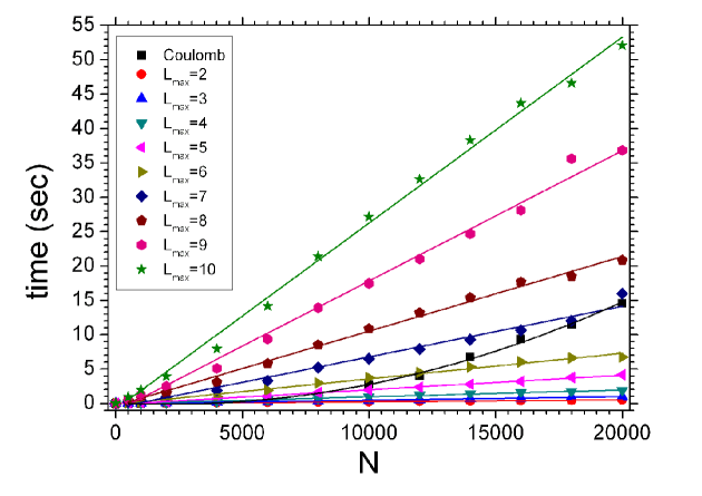
Figure 1: Time needed for energy calculation as a function of the system size.

In Fig. 1 we present the dependencies of the computer time needed for the CE calculation (squares) and for the computation of energy within the TCM method for different values of the principal multipole number as a function of system size. This data was obtained on a 1.8 GHz 64-bit AMD Opteron-244 computer.

From Fig. 1 it is clear that the time needed for the CE calculation has a prominent parabolic trend that is consistent with the analytical expression (10). The fitting expression which describes this dependance is given in the first row of Tab. 1. At large $N$ the $N^{2}$ term becomes dominant and the other two terms can be neglected. Thus, $\alpha_{Coul}\approx 4.46\cdot 10^{-8}$ $(sec)$.

Table 1: Fitting expressions for the computational time needed for the CE calculation and for the energy computation within the TCM method at different values of the principal multipole number, $L_{max}$ (second column). System sizes, for which the Coulomb energy calculation becomes more computer time demanding at a given value of $L_{max}$ are shown in the third column.

$L_{max}$	$\tau(N)$ (sec.)	$N_{max}$
Coulomb	$0.11736-0.0002N+4.6768\cdot 10^{-8}N^{2}$	-
2	$-0.01986+3.0\cdot 10^{-5}N$	4223
3	$-0.03159+5.0\cdot 10^{-5}N$	4662
4	$-0.04714+1.0\cdot 10^{-4}N$	5809
5	$-0.16054+2.1\cdot 10^{-4}N$	8026
6	$-0.14710+3.7\cdot 10^{-4}N$	11704
7	$-0.59675+7.4\cdot 10^{-4}N$	19308
8	$-0.35383+10.9\cdot 10^{-4}N$	27212
9	$-1.15856+1.9\cdot 10^{-3}N$	44286
10	$-0.83688+2.71\cdot 10^{-3}N$	61892

The fitting expressions which describe the time needed for the energy computations within the TCM method at different values of the principal multipole number are given in Tab. 1, rows 2-10. These expressions were obtained by fitting the data shown in Fig. 1. Note the linear dependence on $N$. The numerical coefficient in all expressions correspond to the factor $\alpha_{mult}L_{max}(1+L_{max})^{3}$ in equation (III.1). The fitting expressions in Tab. 1 were obtained by fitting of data obtained for systems with large number of particles (see Fig. 1). Therefore these expressions are applicable when $N\gg 1$.

From equations presented in Tab. 1 it is possible to determine the critical system sizes at which the TCM method becomes less computer time demanding then the CE calculation. The critical system sizes calculated for different principal multipole numbers are shown in the third column of Tab. 1. These sizes correspond to the intersection points of the parabola describing the time needed for the CE calculation with the straight lines describing the computational time needed for the TCM method. In Fig. 1 one can see six intersection points for $L_{max}=2-7$.

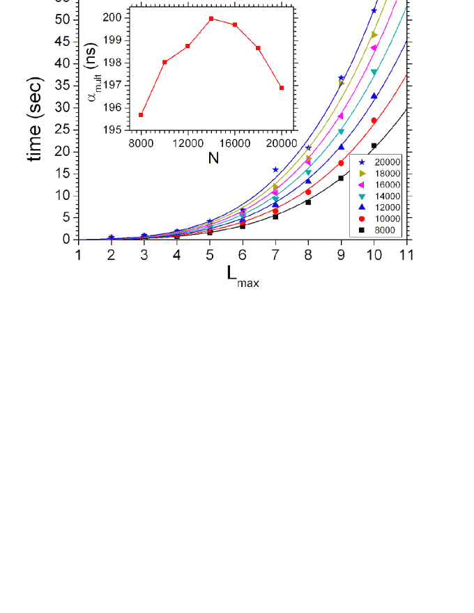
Figure 2: Time needed for the calculation of energy of the systems of different sizes computed within the framework of the TCM method as a function of the principal multipole number $L_{max}$. In the inset we plot $\alpha_{mult}$ as a function of the system size.

From equation (III.1), it follows that computation time of the energy within the framework of the TCM method grows as the power of 4 with increasing $L_{max}$. To stress this fact, in Fig. 2 we present the dependencies of the computation time obtained within the TCM method at different system sizes as a function of principal multipole number. All curves shown in Fig. 2 can be perfectly fitted by the analytical expression (III.1). In the inset to Fig. 2, we plot the dependence of the fitting coefficient $\alpha_{mult}$ as a function of the system size. From this plot it is seen that $\alpha_{mult}$ varies only slightly for all system sizes considered, being equal to $(1.982\pm 0.015)\cdot 10^{-7}$ $(sec)$.

Thus, the expression for the time needed for the energy calculation within the framework of the TCM method reads as:

$$\tau_{mult}(L_{max})\approx 1.98\cdot 10^{-7}L_{max}(1+L_{max})^{3}N.$$ (12)

Note, that $\alpha_{mult}=1.98\cdot 10^{-7}$ $(sec)$ is larger than $\alpha_{Coul}\approx 4.46\cdot 10^{-8}$ $(sec)$, since in one turn of the TCM method more algebraic operations have to be done, than in one turn of the CE calculation.

From the analysis performed in this section it is clear that the TCM method can give a significant gain in the computation time. However, at larger principal multipole numbers ($L_{max}=8,9,10$) this method can compete with the CE calculation only at system sizes greater than 27000-61000 atoms. The accounting for higher multipoles is necessary if the distance between two interacting systems becomes comparable to the size of the systems. In the next section we discuss in detail the accuracy of the TCM method and identify situations in which higher multipoles should be accounted for.

III.2 Comparison with the fast multipole method

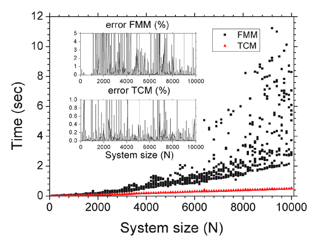
Figure 3: Time needed for the calculation of the interaction energy between two systems as a function the total number of particles calculated within the framework of the TCM method (triangles) and within the framework of the FMM (squares). In the upper and lower insets we plot the relative error of the FMM and of the TCM methods as a function of the system size respectively.

The fast multipole method (FMM) Greengard85 ; Boar2000 ; Pincus77 is a well known method for calculating the electrostatic energy in a multiparticle system, which provides a linear scaling of the computing time with the system size. In order to stress the computational efficiency of the TCM method in this section we compare the time required for the energy calculation within the framework of the FMM and using the TCM method.

To perform such a comparison we used an adaptive FMM library, which has been implemented for the Coulomb potential in three dimensions Gibbon02 ; FMMcode . We have generated two random charge distributions of different size and calculated the interaction energies between them as well as the required computation time using the FMM and the TCM methods. As in the previous section the charges in both systems were randomly distributed within the spheres of radii $R_{A}=1.0\cdot N_{A}^{1/3}$ and $R_{B}=1.0\cdot N_{B}^{1/3}$ respectively and the distance between the center of mass of the two systems was chosen as $R_{0}=3/2(R_{A}+R_{B})$.

In Fig. 3 we present the comparison of the computer time needed for the FMM calculation (squares) and for the computation of energy within the TCM method (triangles) as a function of system size. These data were obtained on an Intel(R) Xeon(TM) CPU 2.40GHz computer. In the upper and lower insets of Fig. 3 we show the relative error of the FMM and of the TCM methods as a function of the system size respectively, which is defined as follows:

$$\eta_{method}=\frac{|U_{coul}-U_{method}|}{|U_{coul}|}\cdot 100\%.$$ (13)

Here $method$ indicates the FMM or the TCM methods. For comparing the efficiency of the two methods we have considered different charge distributions within the size range of 100 to 10000 particles. Each point in Fig. 3 corresponds to a particular charge distribution. For each system size ten different charge distributions were used. The time of the FMM calculation depends on the charge distribution, as is clearly seen in Fig. 3. Note that for a given system size the calculation time of the FMM can change by more than a factor of 5, depending on the charge distribution (see points for $N=10000$ in Fig. 3).

For all system sizes FMM requires some minimal computer time for calculating the energy of the system, which increases with the growth of system size (see Fig. 3). The comparison of the minimal FMM computation time with the computation time required for the TCM method shows that the TCM method appears to be significantly faster than the FMM. For $N=10000$ FMM requires at least 2.15 seconds to compute the energy, while TCM method requires 0.53 seconds, being approximately 4 times faster.

The results of the TCM method calculation shown in Fig. 3, were obtained for $L_{max}=2$. The analysis of relative errors presented in the inset to Fig. 3 shows that with this principal multipole number it is possible to calculate the energy between two systems with an error of less than 1 % for almost arbitrary charge distribution. Note that for the same charge distributions the error of the FMM is much more, being about 5 % in almost all of the considered systems. This allows us to conclude that the TCM method is more efficient and more accurate than the classical FMM.

It is important to mention that in the traditional implementation, FMM calculates the total electrostatic energy of the system while TCM method was developed for studying interaction energy between system fragments. It is possible to modify the FMM to study only interaction energies between different parts of the system. However, the computation cost of the modified FMM is expected to be higher than of the TCM method. This happens because, within the framework of the modified FMM method, the field created by one fragment of the system should be expanded in the multipole series and the interactions of the resulting multipole moments with the charges from another fragment should be calculated. Thus the computation cost of this method will be proportional to $N_{A}\cdot N_{B}$, where $N_{A}$ and $N_{B}$ are the number of particles in two fragments, while the TCM method is proportional to $N_{A}+N_{B}$. The computation cost of the modified version of the FMM depends quadratically on the size of the system, because in this method the interacting fragments should be considered as two independent cells, while traditional FMM uses a hierarchical subdivision of the whole system into cells to achieve linear scaling.

So far we have considered only the interaction between two multi particle systems in vacuo, and demonstrated the efficiency of the TCM method in this case, although the TCM method can also be applied to the larger number of interacting systems. The study of structure and dynamics of biomolecular systems consisting of several components (i.e an ensemble of proteins, DNA, macromolecules in solution) is a separate topic, which is beyond the scope of this paper and deserves a separate investigation.

IV Accuracy of the TCM method. Potential energy surface for porcine pancreatic trypsin/soybean trypsin inhibitor complex.

We have calculated the interaction energy between two proteins within the framework of the TCM method and compared it with the exact Coulomb energy value. On the basis of this comparison we have concluded about the accuracy of the TCM method.

In the present paper we have studied the interaction energy between the porcine pancreatic trypsin and the soybean trypsin inhibitor proteins (Protein Data Bank (PDB) Protbase entry 1AVW Song98 ). Trypsins are digestive enzymes produced in the pancreas in the form of inactive trypsinogens. They are then secreted into the small intestine, where they are activated by another enzyme into trypsins. The resulting trypsins themselves activate more trypsinogens (autocatalysis). Members of the trypsin family cleave proteins at the carboxyl side (or ”C-terminus”) of the amino acids lysine and arginine. Porcine pancreatic trypsin is a archetypal example. Its natural non-covalent inhibitor (porcine pancreatic trypsin inhibitor) inhibits the enzyme’s activity in the pancreas, protecting it from self-digestion.

Trypsin is also inhibited non-covalently by the soybean trypsin inhibitor from the soya bean plant, although this inhibitor is unrelated to the porcine pancreatic trypsin inhibitor family of inhibitors. Although the biological function of the soybean trypsin inhibitor is mostly unknown it is assumed to help defend the plant from insect attack by interfering with the insect digestive system.

The structure of both proteins is shown in Fig. 4. The coordinate frame used for our computations is marked in the figure. This coordinate frame is consistent with the standard coordinate frame used in the PDB.

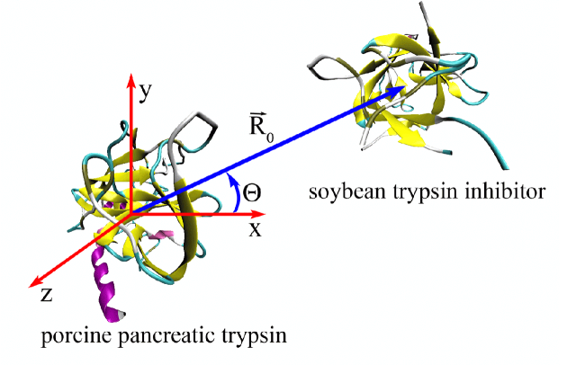
Figure 4: Structure of the porcine pancreatic trypsin and soybean trypsin inhibitor with the coordinate frame used for the energy computation. Figure has been rendered with help of the VMD visualization package Humphrey96

We use this particular example as a model system in order to demonstrate the possible use of the TCM method. Therefore environmental effects are omitted and we consider only the protein-protein interaction in vacuo. The porcine pancreatic trypsin and the soybean trypsin inhibitor include 223 and 177 amino acids respectively. Both proteins include 5847 atoms. Thus for such system size the TCM method is faster than the CE calculation if $L_{max}\leq 4$ (see Tab. 1).

We have calculated the interaction energy between the porcine pancreatic trypsin and soybean trypsin inhibitor as a function of distance between the centers of masses of the fragments, ${\vec{R}_{0}}$, and the angle $\Theta$, which is determined as the angle between the x-axis and the vector ${\vec{R}_{0}}$ (see Fig. 4). We have assumed that the porcine pancreatic trypsin is fixed in space at the center of the coordinate frame and have restricted ${\vec{R}_{0}}$ to the (xy)-plane. Of course, the two degrees of freedom considered are not sufficient for a complete description of the mutual interaction between the two systems. For this purpose at least six degrees of freedom are needed. However for our example of the energy calculation of the porcine pancreatic trypsin/soybean trypsin inhibitor complex within the framework of the TCM method the two coordinates ${\vec{R}_{0}}$ and $\Theta$ are sufficient.

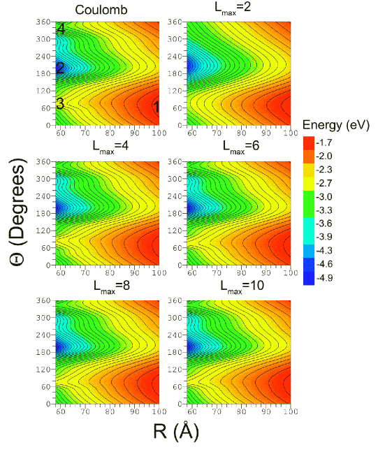
Figure 5: The interaction energies of the porcine pancreatic trypsin with the soybean trypsin inhibitor calculated as the function of $R_{0}$ and $\Theta$ (see Fig. 4) within the framework of the TCM method at different values of the principal multipole number, $L_{max}$. The principal multipole number is given above the corresponding image. The result of the CE calculation is shown in the top left plot.

The interaction energy of the porcine pancreatic trypsin with the soybean trypsin inhibitor as the function of $R_{0}$ and $\Theta$ calculated within the framework of the TCM method is shown in Fig. 5. The Coulomb interaction energy between the two proteins is shown in the top-left plot. In SYSG06_JETP_frag it has been shown that the interaction energy between two well separated biological fragments arises mainly due to the Coulomb forces. In the present paper we consider $R_{0}\in[58,100]$ Å and $\Theta\in[0,360]^{\circ}$, at which condition (2) holds and both proteins can be considered as separated. This means that the potential energy surface shown in the top-left plot of Fig. 5 describes the interaction energy between the porcine pancreatic trypsin and the soybean trypsin inhibitor on the level of accuracy of 90 % at least.

The top-left plot of Fig. 5 shows that one can select several characteristic regions on the potential energy surface marked with numbers 1-4. The corresponding configurations (states) of the system are shown in Fig. 6. The potential energy surface is determined by the Coulomb interactions between atoms, thus at large distances it raises and asymptotically approaches to zero. State 1 has the maximum energy within the considered part of the potential energy surface because this state corresponds to the largest contact separation distance between porcine pancreatic trypsin and the soybean trypsin inhibitor being equal to 54.8 Å.

At smaller distances the potential energy decreases due to the attractive forces acting between the two proteins. State 2 corresponds to the minimum on the potential energy surface. It arises because a positively charged polar arginine (R125) from the porcine pancreatic trypsin approaches the negatively charged site of the soybean trypsin inhibitor, which includes negatively charged polar amino acids glutamic acid (E549) and aspartic acid (D551) (see state 2 in Fig. 6). The strong attraction between the amino acids leads to the formation of a potential well on the potential energy surface. This observation is essential for dynamics of the attachment process of two proteins, because it establishes the most probable angle at which the proteins stick in the (xy)-plane of the considered coordinate frame ($\Theta=192^{\circ}$).

States 3 and 4 correspond to the saddle points on the potential energy surface and have energies higher than state 2. They are formed because at these configurations two positively charged polar amino acids from the two proteins become closer in space providing a source of a local repulsive force. In state 3 these amino acids are lysines (K145 and K665) (see state 3 in Fig. 6), and in state 4 these are arginines (R62 and R563)(see state 4 in Fig. 6).

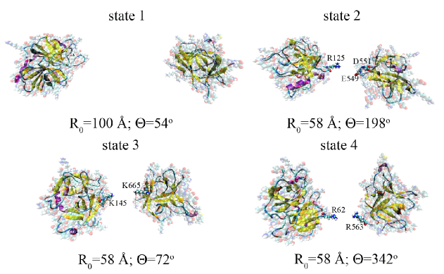
Figure 6: Relative orientations of the porcine pancreatic trypsin and the soybean trypsin inhibitor, corresponding to the selected points on the potential energy surface presented in Fig. 5. Below each image we give the corresponding values of $R_{0}$ and $\Theta$. Some important amino acids are marked according to their PDB id. Figure prepared with help of the VMD visualization package Humphrey96

In the top-right plot of Fig. 5 we present the potential energy surface obtained within the framework of the TCM method with $L_{max}=2$, i.e. with accounting for up to the quadrupole-quadrupole interaction term in the multipole expansion (9). From the figure it is seen that the TCM method describes correctly the major features of the potential energy landscape (i.e. the position of the minimum and maximum as well as their relative energies). However, the minor details of the landscape, such as the saddle points 3 and 4 (see top-left plot of Fig. 5) are missed.

The relative error of the TCM method can be defined as follows:

$$\eta(L_{max})(R_{0},\Theta)=\frac{|U_{coul}(R_{0},\Theta)-U_{mult}^{L_{max}}(R_{0},\Theta)|}{|U_{coul}(R_{0},\Theta)|}\cdot 100\%,$$ (14)

where $U_{coul}(R_{0},\Theta)$ and $U_{mult}^{L_{max}}(R_{0},\Theta)$ are the Coulomb energy and the energy calculated at given values of $R_{0}$ and $\Theta$ within the TCM method respectively. In the top-left plot of Fig. 7 we present the relative error calculated according to (14) for $L_{max}=2$. From this plot it is clear that significant deviation from the exact result arise at $\Theta\sim 50-60^{\circ}$, $140-150^{\circ}$, $245^{\circ}$, $300-310^{\circ}$ and $350^{\circ}$. The discrepancy at $\Theta\sim 50-60^{\circ}$, $\Theta\sim 300-310^{\circ}$ and $\Theta\sim 350^{\circ}$ arises because the saddle points 3 and 4, can not be described within the framework of TCM method with $L_{max}=2$. The discrepancy at $\Theta\sim 140-150^{\circ}$ and $\Theta\sim 245^{\circ}$ is due to the error in the calculation of the slopes of minimum 2 at $R_{0}=58$ Å and $\Theta=198^{\circ}$.

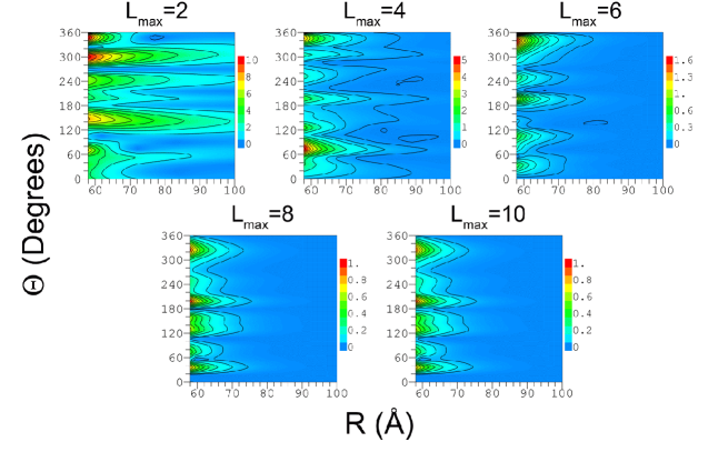
Figure 7: Relative error of the interaction energies of the porcine pancreatic trypsin with the soybean trypsin inhibitor calculated as the function of $R_{0}$ and $\Theta$ within the framework of the TCM method at different values of the principal multipole number, $L_{max}$. The principal multipole number is given above the corresponding image.

It is worth noting that the relative error of the TCM method with $L_{max}=2$ is less than 10 %. With increasing distance between the proteins, the relative error decreases, and becomes less than 5 % at $R_{0}\geq 72$ Å and less than 3 % at $R_{0}\geq 86$ Å. This means that already at $L_{max}=2$ the TCM method reproduces with a reasonable accuracy the essential features of the potential energy landscape. This observation is very important, because TCM method with $L_{max}=2$ requires less computer time then the CE calculation already at $N=4223$ (see Tab. 1). Thus, the TCM method can be used for the identification of major minima and maxima on the potential energy surface of macromolecules and modeling dynamics of complex molecular systems.

Accounting for higher multipoles in the multipole expansion (9) leads to a more accurate calculation of the potential energy surface. In the second row of Fig. 5 we present the potential energy surfaces obtained within the framework of the TCM method with $L_{max}=4$ and $6$. From these plots it is seen that all minor details of the Coulomb potential energy surface, such as the saddle points 3 and 4 are reproduced correctly. Figure 7 shows that the TCM method with $L_{max}=4$ gives the maximal relative error of about 5 % at $R_{0}=58$ Å and $\Theta=75^{\circ}$, in the vicinity of the saddle point 3. The relative errors in the vicinity of the saddle point 4 and minimum 2 are equal to 4 % and 1 % respectively. The error becomes less then 1 % for all values of angle $\Theta$ at $R_{0}\geq 70$ Å. For $L_{max}=6$, the largest relative error is equal to $1.5$ % at $R_{0}=58$ Å and $\Theta=340^{\circ}$ (saddle point 4), becoming less then 1 % at $R_{0}\geq 61$ Å.

By accounting for the higher multipoles in the multipole expansion (9) one can increase the accuracy of the method. Thus, with $L_{max}=8$ and $10$ it is possible to calculate the potential energy surface with the error less then 1 % (see bottom row in Fig. 5 and Fig. 7). Although the time needed for computing the potential energy surfaces with $L_{max}=8$ and $10$ is larger than the time needed for computing the Coulomb energy directly (see Tab. 1), we present these surfaces in order to stress the convergence of the TCM method.

V Conclusion

In the present paper we have proposed a new method for the calculation of the Coulomb interaction energy between pairs of macromolecular objects. The suggested method provides a linear scaling of the computational costs with the size of the system and is based on the two center multipole expansion of the potential. Analyzing the dependence of the required computer time on the system size, we have established the critical sizes at which our method becomes more efficient than the direct calculation of the Coulomb energy.

The comparison of efficiency of the TCM method with the efficiency of FMM allows us to conclude that the TCM method has proved to be faster and more accurate than the classical FMM.

The method based on the two center multipole expansion can be used for the efficient computation of the interaction energy between complex macromolecular systems. To determine that we have considered the interaction between two proteins: porcine pancreatic trypsin and the soybean trypsin inhibitor. The accuracy of the method has been discussed in detail. It has been shown that accounting of only four multipoles in both proteins gives an error in the interaction energy less than 5 %.

The TCM method is especially useful for studying dynamics of rigid molecules, but it can also be adopted for studying dynamics of flexible molecules. In this work we have developed a method for the efficient calculation of the interaction energy between pairs of large multi particle systems, e.g. macromolecules, being in vacuo. The investigation of biomolecular systems consisting of several components (i.e complexes of proteins, DNA, macromolecules in solution) and the extension of the TCM method for these cases deserves a separate investigation. If a system of interest consists of several interacting molecules being placed in a solution, one can use the TCM method to describe the interaction between the molecules and then to take account of the solution as implicit solvent. This can be achieved using for example the formalism of the Poisson-Bolzmann Fogolari99 ; Baker01 , similar to how it was implemented for the description of the antigen-antibody binding/unbinding process ElsaPoster ; ElsaPaper . The other possibility is to split the whole system into boxes and account for the solvent explicitly by calculating the interactions between the boxes and the molecules of interest. This can be achieved by using the TCM method or a combination of the FMM and the TCM methods. In this case the FMM can be used for the calculation of the resulting effective multipole moment of the solvent, while the TCM method is much better suitable for the description of the macromolecules energetics and dynamics. Note that all of the suggested methodologies provide linear scaling of the computation time on the system size.

The results of this work can be utilized for the description of complex molecular systems such as viruses, DNA, protein complexes, etc and their dynamics. Many dynamical features and phenomena of these systems are caused by the electrostatic interaction between their various fragments and thus the use of the two center multipole expansion method should give a significant gain in their computation costs.

VI Acknowledgements

This work is partially supported by the European Commission within the Network of Excellence project EXCELL and by INTAS under the grant 03-51-6170. We are grateful to Dr. Paul Gibbon for providing us with the FMM code. We thank Dr. Axel Arnold for his help with compiling the programs as well as for many insightful discussions. We also thank Dr. Elsa Henriques and Dr. Andrey Korol for many useful discussions. We are grateful to Ms. Stephanie Lo for her help in proofreading of this manuscript. The possibility to perform complex computer simulations at the Frankfurt Center for Scientific Computing is also gratefully acknowledged.

References

- (1) P.L. Freddolino, A.S. Arkhipov, S.B. Larson, A. McPherson, and K. Schulten, Structure 14, 437 (2006).
- (2) A.Y. Shih, A. Arkhipov, P.L. Freddolino, and K. Schulten., Journ. Phys. Chem. B 110, 3674 (2006).
- (3) D. Lu, A. Aksimentiev, A.Y. Shih, E. Cruz-Chu, P.L. Freddolino, A. Arkhipov, and K. Schulten, Phys. Biol. 3, S40 (2006).
- (4) H. Meyer and J. Baschnagel, Eur. Phys. Jorn. E 12, 147 (2003).
- (5) A.V. Yakubovich, I.A. Solov’yov, A.V. Solov’yov and W. Greiner, Eur. Phys. Journ. D 39, 23 (2006).
- (6) I.A. Solov’yov, A.V. Yakubovich, A.V. Solov’yov and W. Greiner, Phys. Rev. E 73 021916 (2006)
- (7) I.A. Solov’yov, A.V. Yakubovich, A.V. Solov’yov and W. Greiner, Journ. of Exp. and Theor. Phys. 102, 314 (2006). Original Russian Text, published in Zh. Eksp. Teor. Fiz. 129, 356 (2006).
- (8) I.A. Solov’yov, A.V. Yakubovich, A.V. Solov’yov and W. Greiner, Journ. of Exp. and Theor. Phys. 103, 463 (2006). Original Russian Text, published in Zh. Eksp. Teor. Fiz. 130, 534 (2006).
- (9) A.V. Yakubovich, I.A. Solov’yov, A.V. Solov’yov and W. Greiner, Eur. Phys. Journ. D, 40 363 (2006), (Highlight paper).
- (10) C. Chen, Y. Xiao, L. Zhang, Biophysical Journal 88, 3276 (2005).
- (11) Y. Duan, P. A. Kollman, Science 282 740 (1998).
- (12) A. Liwo, M. Khalili and H. A. Scheraga, PNAS 102, 2362 (2005).
- (13) F. Ding, N. V. Dokholyan, S. V. Buldyrev, H. E. Stanley and E. I. Scakhnovich, Biophysical Journal 83, 3525 (2002).
- (14) E.S. Henriques and A.V. Solov’yov, Abstract at the WE-Heraeus- Seminar ”Biomolecular Simulation: From Physical Principles to Biological Function”. Manuscript in preparation (2006).
- (15) E.S. Henriques and A.V. Solov’yov, submitted to Europhys. J. D (2007).
- (16) W.F. van Gunsteren and H.J.C. Berendsen, Angew. Chem. Int. Ed. Engl. 29, 992 (1990).
- (17) H.G. Petersen, D. Soelvason and J.W. Perram, J. Chem. Phys. 101, 8870 (1994).
- (18) H.-Q. Ding, N. Karasawa, and W.A. Goddard III, J. Chem. Phys. 97, 4309 (1992).
- (19) C.A. White, B.G. Johnson, P.M.W. Gill, M. Head-Gordon, Chem. Phys. Lett. 230, 8 (1994).
- (20) K.E. Schmidt and M.A. Lee, Journ. of Stat. Phys. 63, 1223 (1991).
- (21) L. Grengard and V. Rokhlin, J. Comput. Phys. 60, 187 (1985).
- (22) J. Board and K. Schulten, Comp. Sci. Eng., 56 (2000)
- (23) M.R. Pincus and H.A. Scheraga, J. Phys. Chem. 81, 1579 (1977).
- (24) P. Gibbon and G. Sutmann, in Quantum Simulations of Complex Many-Body Systems: From Theory to Algorithms, Lecture Notes, J. Grotendorst, D. Marx, A. Muramatsu (Eds.), John von Neumann Institute for Computing, Jülich, NIC Series 10 467 (2002).
- (25) J.A. Board, J.W. Causey, J.F. Leathrum, Jr., A. Windemuth, and K. Schulten, Chem. Phys. Lett. 198, 89 (1992);
- (26) F. Zhao and S.L. Johnson, Siam. J. Sci. Stat. Comput. 12, 1420 (1991).
- (27) J. Shimada, H. Kaneko, and T. Takada, J. Comp. Chem. 15, 29 (1994).
- (28) R.J. Buehler and J.O. Hirschfelder, Phys. Rev. 83, 628 (1951).
- (29) C.G. Joslin and C.G. Gray, J.Phys.A: Mat. Gen 17, 1313 (1984).
- (30) G.P. Gupta and K.C. Mathur, Phys. Rev. A 23, 2347 (1981).
- (31) W.P Wolf and R.J. Birgeneau, Phys. Rev. 166, 376 (1968).
- (32) D.A. Varshalovich, A.N. Moskalev, and V.K. Khersonskii, Qunatum Theory of Angular Momentum (World Scientific, Singapore, 1988).
- (33) The FMM library for long range Coulomb interactions was provided by the complex atomistic modeling and simulations group, Forschungszentrum Jülich, http://www.fz-juelich.de/zam/fcs/
- (34) F. Fogolari, P. Zuccato, G. Esposito, and P. Viglino, Biophys. J. 76, 1 (1999).
- (35) N.A. Baker, D. Sept, S. Joseph, M.J. Holst and J.A. MacCammon, Proc. Natl. Acad. Sci 98, 10037 (2001).
- (36) H. Berman, J. Westbrook, Z. Feng, G. Gilliland, T. Bhat, H. Weissig, I. Shindyalov, P. Bourne, Nucleic Acids Research 28, 235 (2000).
- (37) H.K. Song and S.W. Suh, Journ. of Mol. Biol. 275, 347 (1998).
- (38) W. Humphrey, A. Dalke and K. Schulten, Journ. Molec. Graphics 14.1, 33 (1996)