Spectral Analysis of the Chandra Comet Survey

Abstract

Aims. We present results of the analysis of cometary X-ray spectra with an extended version of our charge exchange emission model (Bodewits et al. 2006). We have applied this model to the sample of 8 comets thus far observed with the Chandra X-ray observatory and acis spectrometer in the 300–1000 eV range. The surveyed comets are C/1999 S4 (linear), C/1999 T1 (McNaught–Hartley), C/2000 WM1 (linear), 153P/2002 (Ikeya–Zhang), 2P/2003 (Encke), C/2001 Q4 (neat), 9P/2005 (Tempel 1) and 73P/2006-B (Schwassmann–Wachmann 3) and the observations include a broad variety of comets, solar wind environments and observational conditions.

Methods. The interaction model is based on state selective, velocity dependent charge exchange cross sections and is used to explore how cometary X-ray emission depend on cometary, observational and solar wind characteristics. It is further demonstrated that cometary X-ray spectra mainly reflect the state of the local solar wind. The current sample of Chandra observations was fit using the constrains of the charge exchange model, and relative solar wind abundances were derived from the X-ray spectra.

Results. Our analysis showed that spectral differences can be ascribed to different solar wind states, as such identifying comets interacting with (I) fast, cold wind, (II), slow, warm wind and (III) disturbed, fast, hot winds associated with interplanetary coronal mass ejections. We furthermore predict the existence of a fourth spectral class, associated with the cool, fast high latitude wind.

1 Introduction

When highly charged ions from the solar wind collide on a neutral gas, the ions get partially neutralized by capturing electrons into an excited state. These ions subsequently decay to the ground state by the emission of one or more photons. This photon emission is called charge exchange emission (cxe) and it has been observed from comets, planets and the interstellar medium in X-rays and the Far-UV Lisse et al. (1996); Krasnopolsky (1997); Snowden et al. (2004); Dennerl (2002). The spectral shape of the cxe depends on properties of both the neutral gas and the solar wind and the subsequent emission can therefore be regarded as a fingerprint of the underlying interactions Cravens et al. (1997); Kharchenko and Dalgarno (2000, 2001); Beiersdorfer et al. (2003); Bodewits et al. (2004a, 2006).

Since the first observations of cometary X-ray emission, more than 20 comets have been observed with various X-ray and Far-UV observatories Lisse et al. (2004); Krasnopolsky et al. (2004). This observational sample contains a broad variety of comets, solar wind environments and observational conditions. The observations clearly demonstrate the diagnostics available from cometary charge exchange emission.

First of all, the emission morphology is a tomography of the distribution of neutral gas around the nucleus Wegmann et al. (2004). Gaseous structures in the collisionally thin parts of the coma brighten, such as the jets in 2P/Encke Lisse et al. (2005), the Deep Impact triggered plume in 9P/Tempel 1 Lisse et al. (2007) and the unusual morphology of comet 6P/d’Arrest Mumma et al (1997). In other comets, the X-ray emission clearly mapped a spherical gas distribution. This resulted in a characteristic crescent shape for larger and hence collisionally thick comets observed at phase angles of roughly 90 degrees (e.g. Hyakutake - Lisse et al. (1996), linear S4 - Lisse et al. (2001)). Macroscopic features of the plasma interaction such as the bowshock are observable, too Wegmann & Dennerl (2005).

Secondly, by observing the temporal behavior of the comet s X-ray emission, the activity of the solar wind and comet can be monitored. This was first shown for comet C/1996 B2 (Hyakutake) Neugebauer et al. (2000) and recently in great detail by long term observations of comet 9P/2005 (Tempel 1) Willingale et al. (2006); Lisse et al. (2007) and 73P/2006 (Schwassmann–Wachmann 3C) Brown et al. (2007), where cometary X-ray flares could be assigned to either cometary outbursts and/or solar wind enhancements.

Thirdly, cometary spectra reflect the physical characteristics of the solar wind; e.g. spectra resulting from either fast, cold (polar) wind and slow, warm equatorial solar wind should be clearly different Schwadron and Cravens (2000); Kharchenko and Dalgarno (2001); Bodewits et al. (2004a). Several attempts were made to extract ionic abundances from the X-ray spectra.

The first generation spectral models have all made strong assumptions when modelling the X-ray spectra Haeberli et al (1997); Wegmann et al. (1998); Kharchenko and Dalgarno (2000); Schwadron and Cravens (2000); Lisse et al. (2001); Kharchenko and Dalgarno (2001); Krasnopolsky et al. (2002); Beiersdorfer et al. (2003); Wegmann et al. (2004); Bodewits et al. (2004a); Krasnopolsky (2004); Lisse et al. (2005). Here, we present a more elaborate and sophisticated procedure to analyze cometary X-ray spectra based on atomic physics input, which for the first time allows for a comparative study of all existing cometary X-ray spectra. In Section 2, our comet-wind interaction model is briefly introduced. In Section 3, it is demonstrated how cometary spectra are affected by the velocity and target dependencies of charge exchange reactions. In Section 4, the various existing observations performed with the Chandra X-ray Observatory, as well as the solar wind data available are introduced. Based upon our modelling, we construct an analytical method of which the details and results are presented in Section 5. In Section 6, we discuss our results in terms of comet and solar wind characteristics. Lastly, in Section 7 we summarize our findings. Details of the individual Chandra comet observations are given in Appendix A.

2 Charge Exchange Model

2.1 Atomic structure of He-like ions

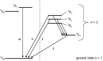
Figure 1: Part of the decay scheme of a helium–like ion. The ¹S₀ decays to the ground state via two-photon processes (not indicated).

Electron capture by highly charged ions populates highly excited states, which subsequently decay to the ground state. These cascading pathways follow ionic branching ratio statistics. Because decay schemes work as a funnel, the lowest transitions ($n=2\to 1$) are the strongest emission lines in cxe spectra. For helium-like ions, these are the forbidden line ($z$: 1s^2 1S₀–1s2s ³S₁), the intercombination lines ($y,x$: 1s^2 1S₀–1s2p ³P_1,2), and the resonance line (w: 1s^2 1S₀–1s2p ¹P₁), see Figure 1.

The apparent branching ratio, B_eff, for the intercombination transitions is determined by weighting branching ratios (B_j) derived from theoretical transition rates compiled by Porquet et al. (2000, 2001), by an assumed statistical population of the triplet P-term:

$$B_{\mathrm{eff}}=\sum^{2}_{j=0}\frac{(2j+1)}{(2L+1)(2S+1)}\cdot\mathrm{B}_{j}$$ (1)

The resulting effective branching ratios are given in Table 1. These ratios can only be observed at conditions where the metastable state is not destroyed (e.g. by UV flux or collisions) before it decays. In contrast to many other astrophysical X-ray sources, this condition is fulfilled in cometary atmospheres, making the forbidden lines strong markers of cxe emission.

Table 1: Apparent effective branching ratios (B_eff) for the relaxation of the 2³P-state of He-like carbon, nitrogen, oxygen and neon.

transition	C v	N vi	O vii	Ne ix
1s2 (1S0)–1s2p (3P1,2)	0.11	0.22	0.30	0.34
1s2s (3S1)–1s2p (3P${}_{0,1,2})$	0.89	0.78	0.70	0.66

2.2 Emission Cross Sections

To obtain line emission cross sections we start with an initial state population based on state selective electron capture cross sections and then track the relaxation pathways defined by the ion’s branching ratios.

Table 2: Compilation of theoretical, velocity dependent emission cross sections for collisions between bare- and H-like solar wind ions and atomic hydrogen, in units of 10^-16 cm². See text for details. We estimate uncertainties to be ca. 20%. The ion column contains the resulting ion, not the original solar wind ion. Line energies compiled from Garcia & Mack (1965); Vainshtein & Safronova (1985); Drake (1988); Savukov et al. (2003) and the chianti database Dere et al. (1997); Landi et al. (2006).

$E$ (eV)	Ion	Transition	200 km s-1	400 km s-1	600 km s-1	800 km s-1	1000 km s-1
299.0	C v	z	8.7	12	16	18	20
304.4	C v	x,y	0.65	1.0	1.5	1.7	1.8
307.9	C v	w	1.8	3.0	4.1	4.8	5.2
354.5	C v	1s3p-1s2	0.55	0.71	0.81	1.0	1.3
367.5	C v	1s4p-1s2	0.70	0.66	0.76	0.74	0.72
367.5	C vi	2p-1s	15	26	30	33	34
378.9	C v	1s5p-1s2	0.00	0.02	0.05	0.04	0.04
419.8	N vi	z	13	23	28	29	29
426.3	N vi	x,y	2.7	4.3	5.3	5.7	6.0
430.7	N vi	w	3.8	6.0	7.4	8.1	8.5
435.5	C vi	3p-1s	1.6	4.0	4.7	4.7	4.8
459.4	C vi	4p-1s	2.9	5.9	7.0	6.4	6.0
471.4	C vi	5p-1s	0.55	1.0	1.3	0.85	0.54
497.9	N vi	1s3p-1s2	0.43	0.99	1.3	1.3	1.3
500.3	N vii	2p-1s	40	45	44	42	42
523.0	N vi	1s4p-1s2	0.81	1.6	1.9	1.8	1.7
534.1	N vi	1s5p-1s2	0.14	0.31	0.33	0.21	0.14
561.1	O vii	z	37	34	33	32	31
568.6	O vii	x,y	10	10	10	9.9	9.7
574.0	O vii	w	9.9	11	11	11	10
592.9	N vii	3p-1s	6.3	4.9	4.8	4.5	4.3
625.3	N vii	4p-1s	2.9	2.9	3.7	4.3	4.6
640.4	N vii	5p-1s	11	5.2	3.7	2.7	2.2
650.2	N vii	6p-1s	0.00	0.21	0.13	0.09	0.08
653.5	O viii	2p-1s	27	40	48	51	53
665.6	O vii	1s3p-1s2	1.7	1.3	1.3	1.2	1.2
697.8	O vii	1s4p-1s2	0.81	0.79	1.0	1.2	1.3
712.8	O vii	1s5p-1s2	2.8	1.3	0.92	0.68	0.54
722.7	O vii	1s6p-1s2	0.00	0.06	0.04	0.02	0.02
774.6	O viii	3p-1s	2.6	4.7	5.6	5.3	5.0
817.0	O viii	4p-1s	1.0	1.6	2.0	2.2	2.3
836.5	O viii	5p-1s	2.4	4.0	4.6	4.1	3.7
849.1	O viii	6p-1s	1.6	1.6	1.5	1.1	0.67

Electron capture reactions can be strongly dependent on target effects. An important difference between reactions with atomic hydrogen and the other species is the presence of multiple electrons, hence allowing for multiple (mostly double) electron transfer. It has been demonstrated both experimentally and theoretically that double electron capture can be an important reaction channel in multi-electron targets and that after autoionization to an excited state it may contribute to the X-ray emission Ali et al. (2005); Hoekstra et al. (1989); Beiersdorfer et al. (2003); Otranto et al (2006); Bodewits et al. (2006). Unfortunately, experimental data on reactions with species typical for cometary atmospheres, such as H₂O, atomic O and CO are at best scarcely available. Because the first ionization potentials of these species are all close to that of atomic H, using state selective one electron capture cross sections for bare ions charge exchanging with atomic hydrogen from theory is a reasonable assumption, which is also confirmed by experimental studies Greenwood et al. (2000, 2001); Bodewits et al. (2006). Here, we will use the working hypothesis that effective one electron cross sections for multi-electron targets present in cometary atmospheres are at least roughly comparable to cross sections for one electron capture from H. Based on this hypothesis, we will use our comet-wind interaction model to evaluate the contribution of the different species.

For our calculations, we use a compilation of theoretical state selective, velocity dependent cross sections for collisions with atomic hydrogen Errea et al. (2004); Fritsch and Lin (1984); Green et al. (1982); Shipsey et al. (1983). We furthermore assume that capture by H-like ions leads to a statistical triplet to singlet ratio of 3:1, based on measurements by Suraud et al. (1991); Bliek et al. (1998). We will first focus on the strongest emission features, which are the $n=2\to 1$ transitions, i.e., the Ly-$\alpha$ transition (H-like ions) or the forbidden, resonance and intercombination lines (He-like ions).

In Fig. 2, the emission cross sections of the Ly-$\alpha$ or the sum of the emission cross sections of the forbidden, resonance and intercombination lines of different ions (C, N, O) are shown as a function of collision velocity, for one electron capture reactions with atomic hydrogen. This figure sets the stage for solar wind velocity induced effects in cometary X-ray spectra. Most important is the effect of the velocity on the two carbon emission features; their prime emission features increase by a factor of almost two when going from typical ‘slow’ to typical ‘fast’ solar wind velocities. The O viii Ly-$\alpha$ emission cross section can be seen to drop steeply below ca. 300 km s^-1. The N vi K-$\alpha$ displays a similar, though somewhat less strong behavior.

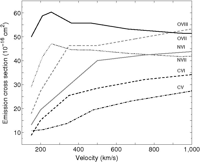
Figure 2: Velocity dependence of Ly-$\alpha$ or the sum of the forbidden/resonance/intercombination emission cross sections of different solar wind ions: O viii (dashed, grey line), O vii (solid, black line), N vii (dotted, black line), N vi (solid, grey line), C vi (dashed, black line) and C v (dash-dotted, black line).

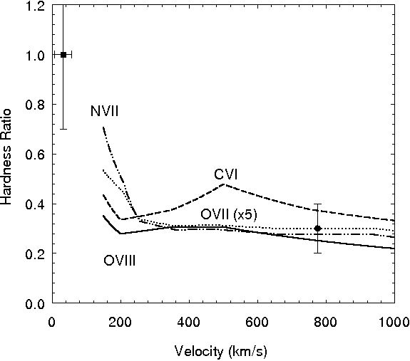
Figure 3: Velocity dependence of the hardness ratio of different solar wind ions: O viii (solid line), O vii (dashed line) N vii (dashed line) and C vi (dash-dotted line). Also shown are two experimentally obtained hardness ratios by Beiersdorfer et al. (2001) and Greenwood et al. (2000) for O⁸⁺ colliding on CO₂ and H₂O, respectively (see text).

The relative intensity of the emission lines (per species) is governed by the state selective electron capture cross sections of the charge exchange reaction and the branching ratios of the resulting ion. A measure of these intensities is the hardness ratio (Beiersdorfer et al. 2001), which is defined as the ratio between the emission cross sections of the higher order terms of the Lyman-series and Ly-$\alpha$ (or between the higher order K-series and K-$\alpha$ in case of He-like ions):

$$\frac{\sum_{n>2}^{\infty}\sigma_{\mathrm{em}}(\mathrm{Ly-}n)}{\sigma_{\mathrm{em}}(\mathrm{Ly-}\alpha)}$$ (2)

For electron capture by H-like ions, we will use the ratio between the sum of the resonance-, intercombination and forbidden emission lines and the rest of the K-series as the hardness ratio. Fig. 3 shows the hardness ratios of cxe from abundant solar wind ions. The figure shows that most hardness ratios are constant at typical solar wind velocities (above 300 km s^-1) but it also clearly demonstrates the suggestion made by Beiersdorfer et al. (2001) that hardness ratios are good candidates for studies of velocimetry deep within the coma when the solar wind has slowed down by mass loading.

2.3 Interaction Model

Cometary high-energy emission depends upon certain properties of both the comet (gas production rate, composition, distance to the Sun) and the solar wind (speed, composition). Recently, we developed a model that takes each of these effects into account Bodewits et al. (2006), which we will briefly describe here.

The neutral gas model is based on the Haser-equation, which assumes that a comet has a spherically expanding neutral coma Haser (1957); Festou (1981). The lifetime of neutrals in the solar radiation field varies greatly amongst species typical for cometary atmospheres Huebner et al. (1992). The dissociation and ionization scale lengths also depend on absolute UV fluxes, and therefore on the distance to the Sun. The coma interacts with solar wind ions, penetrating from the sunward side following straight line trajectories. The charge exchange processes between solar wind ions and coma neutrals are explicitly followed both in the change of the ionization state of the solar wind ions and in the relaxation cascade of the excited ions (as discussed above).

Due to its interaction with the cometary atmosphere, the solar wind is both decelerated and heated in the bow shock. This bow shock does not affect the ionic charge state distribution. The bow shock lowers the drift velocity of the wind but at the same time increases its temperature and the net collision velocity of the ions is ca. 77$\%$ of the initial velocity v$(\infty)$ throughout the interaction zone. We use a rule of thumb derived by Wegmann et al. (2004) to estimate the stand-off distance $R_{\mathrm{bs}}$ of the bow shock.

Deep within the coma, the solar wind finally cools down as the hot wind ions, neutralized by charge exchange, are replaced by cooler cometary ions. For simplicity however, we shall assume that the wind keeps a constant velocity and temperature after crossing the bow shock.

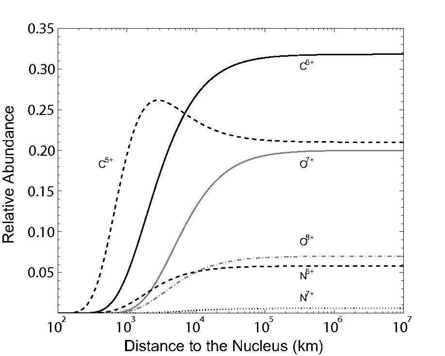
Figure 4: Modeled charge state distribution along the comet-Sun line, assuming an equatorial 300 km s^-1 wind interacting with a comet with outgassing rate Q=$10^{29}$ molecules s^-1 at 1 AU from the Sun. A composition typical for the slow, equatorial wind was assumed.

Initially, the charge state distribution depends on the solar wind state. For most simulation purposes, we will assume the ‘average’ ionic composition for the slow, equatorial solar wind as given by Schwadron and Cravens (2000). Using our compilation of charge changing cross sections, we can solve the differential equations that describe the charge state distribution in the coma in the 2D-geometry fixed by the comet-Sun axis. Figure 4 shows the charge state distribution for a 300 km s^-1 equatorial wind interacting with a comet with an outgassing rate $Q$ of $=10^{29}$ molecules s^-1 comet. From this charge state distribution, it can be seen that along the comet-Sun axis, the comet becomes collisionally thick between 3500 km (O⁸⁺) to 2000 km (C⁶⁺), depending on the cross section of the ions. A maximum in the C⁵⁺ abundance can be seen around 2,000 km, which is due to the relatively large initial C⁶⁺ population and the small cross section of C⁵⁺ charge exchange.

A 3D integration assuming cylindrical symmetry around the comet-Sun axis finally yields the absolute intensity of the emission lines. Effects due to the observational geometry (i.e. field of view and phase angle) are included at this step in the model.

3 Model Results

3.1 Relative Contribution of Target Species

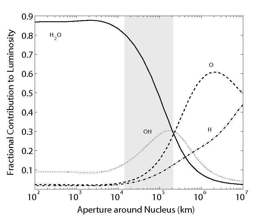
Figure 5: Relative contribution of target species to the total intensity of O vii 570 eV emission complex with increasing field of view, for an active Q$=10^{29}$ molecules s^-1 comet, interacting with a 300 km s^-1 solar wind at 1 AU from the Sun. The shaded area indicates the range of apertures used to obtain spectra discussed within this survey.

Figure 5 shows the dominant collisions which underly the X-ray emission of comets. Shown is the total intensity projected on the sky, with increasing field of view. Within $10^{4}$ km around the nucleus, water is the dominant collision partner. Farther outward ($\geq 2\times 10^{5}$ km), the atomic dissociation products of water take over, and atomic oxygen becomes the most important collision partner. When the field of view exceeds 10⁷ km, atomic hydrogen becomes the sole collision partner. Note that collisions with water never account for 100% of the emission, even with very small apertures, due to the contribution of collisions with atomic hydrogen, OH and oxygen in the line of sight towards the nucleus.

The comets observed with Chandra are all observed with an aperture of ca. 7.5′ centered on the nucleus. This corresponds to a range of $1.6-22\times 10^{4}$ km (as indicated in Figure 5). Our model predicts that the emission from nearby comets will be dominated by cxe from water, but that for comets observed with a larger field of view, up to 60% of the emission can come from cxe interactions with the water dissociation products atomic oxygen and OH, and 10% from interactions with atomic hydrogen.

3.2 Solar Wind Velocity

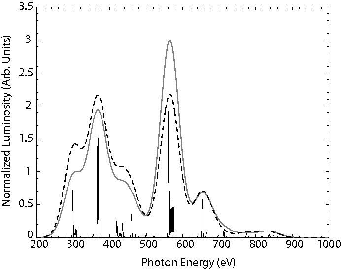
Figure 6: Simulated X-ray spectra for a 10²⁹ molecules s^-1 comet interacting with an equatorial wind with velocities of 300 km s^-1 (solid grey line) and 700 km s^-1 (dashed black line). The spectra are convolved with Gaussians with a width of $\sigma=50$ eV to simulate the Chandra spectral resolution. To indicate the different lines, also the 700 km s^-1 $\sigma=1$ eV spectrum is indicated (not to scale). A field of view of 10⁵ km and ‘typical’ slow wind composition were used.

To illustrate solar wind velocity induced variations in charge exchange spectra, we simulated charge exchange spectra following solar wind interactions between an equatorial wind and a $Q=10^{29}$ molecules s^-1 comet, and assumed the same solar wind composition in all cases. In Fig. 6, spectra resulting from collisional velocities of 300 km s^-1 and 700 km s^-1 are shown. In the spectrum from the faster wind, the C vi 367 eV and O vii 570 eV emission features are roughly equally strong, whereas at 300 km s^-1, the oxygen feature is clearly stronger. Assuming the wind’s composition remains the same, within the range of typical solar wind velocities (300–700 km s^-1), the cross sectional dependence on solar wind velocity does not affect cometary X-ray spectra by more than a factor 1.5. In practice, the compositional differences between slow and fast wind will induce much stronger spectral changes.

3.3 Collisional Opacity

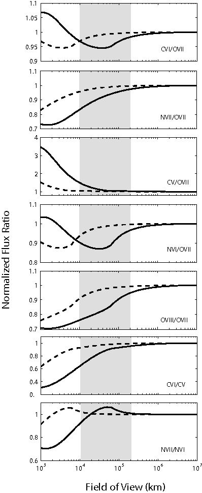
Figure 7: Collisional opacity effects on flux ratios within the field of view. The outer bounds of the fields of view within this survey were between $10^{4}-10^{5}$ km, as indicated by the shaded area. We considered a 500 km s^-1 equatorial wind interacting with comets with different activities: $Q=10^{28}$ molecules s^-1  (dashed lines) and $Q=10^{29}$ molecules s^-1 (solid lines). All flux ratios are normalized to 1 at infinity.

Many of the 20⁺ comets that have been observed in X-ray display a typical crescent shape as the solar wind ion content is depleted via charge exchange. Comets with low outgassing rates around 10²⁸ molecules s^-1, such as 2P/2002 (Encke) and 9P/2005 (Tempel 1), did not display this emission morphology Lisse et al. (2005, 2007). Whether or not the crescent shape can be resolved depends mainly on properties of the comet (outgassing rate), but, to a minor extent, also on the solar wind (velocity dependence of cross sections). Other parameters (secondary, but important), are the spatial resolution of the instrument and the distance of the comet to the observer.

In a collisionally thin environment, the ratio between emission features is the product of the ion abundance ratios and the ratio between the relevant emission cross sections:

$$r_{\mathrm{thin}}=\frac{n(A^{q+})}{n(B^{q+})}\cdot\frac{\sigma_{\mathrm{em}}^{A^{q+}}(\mathrm{v})}{\sigma_{\mathrm{em}}^{B^{q+}}(\mathrm{v})}$$ (3)

The flux ratio for a collisionally thick system depends on the charge states considered. In case of a bare ion $A$ and a hydrogenic ion $B$, the ratio between the photon fluxes from $A$ and $B$ is given by the abundance ratio weighted by efficiency factors $\mu$ and $\eta$:

$$r_{\mathrm{thick}}=\frac{n(A^{q+})}{n(B^{(r-1)+})+\mu(B^{r+})n(B^{r+})}\cdot\frac{\eta(A^{q+})}{\eta(B^{(r-1)+})}$$ (4)

The efficiency factor $\mu$ is a measure of how much B^(r-1)+ is produced by charge exchange reactions by B^q+:

$$\mu=\frac{\sigma_{r,r-1}(\mathrm{v})}{\sigma_{r}(\mathrm{v})}$$ (5)

where $\sigma_{r}$ is the total charge exchange cross section and $\sigma_{r,r-1}$ the one electron charge changing cross section. The efficiency factor $\eta$ describes the emission yield per reaction and is given by the ratio between the relevant emission cross section $\sigma_{\mathrm{em}}$ and the total charge changing cross section $\sigma_{r}$:

$$\eta=\frac{\sigma_{\mathrm{em}}(\mathrm{v})}{\sigma_{r}(\mathrm{v})}$$ (6)

To explore the effect of collisional opacity on spectra, we simulated two comets at 1 AU from the Sun, with gas production rates of $10^{28}$ and $10^{29}$ molecules s^-1, interacting with a solar wind with a velocity of 500 km s^-1 and an averaged slow wind composition Schwadron and Cravens (2000). The results are summarized in Figure 7 where different flux ratios are shown. The behavior of these ratios as a function of aperture is important because they can be used to derive relative ionic abundances. All ratios are normalized to 1 at infinite distance from the comet’s nucleus. For low activity comets with $Q\leq 10^{28}$ molecules s^-1, the collisional opacity does not affect the comet’s X-ray spectrum. Within typical field of views all line flux ratios are close to the collisionally thin value. For more active comets ($Q=10^{29}$ molecules s^-1), collisional opacity can become important within the field of view. Observed flux ratios involving C v should be treated with care, see e.g. C v/O vii and C vi/C v, because the flux ratios within the field of view can be affected by almost 50% and 35%, respectively. The effect is the strongest in these cases because of the large relative abundance of C⁶⁺, that contributes to the C v emission via sequential electron capture reactions in the collisionally thick zones. For N vii and O viii, a small field of view of $10^{4}$ km could affect the observed ionic ratios by some 20%.

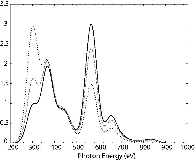
Figure 8: Simulated X-ray spectra for a 10²⁹ molecules s^-1 comet interacting with an equatorial wind with a velocity of 300 km s^-1 for fields of view decreasing from 10⁵ km (solid line), 10⁴ km (dashed line) and 10³ km (dotted line).

To further illustrate these results, we show the resulting X-ray spectra in Fig. 8. There, we consider a $Q=10^{29}$ molecules s^-1 comet interacting with a 300 km s^-1 wind and show the effect of slowly zooming from the collisionally thin to the collisionally thick zone around the nucleus. The field of view decreases from $10^{5}$ to $10^{3}$ km. At $10^{5}$ km, the spectrum is not affected by collisionally thick emission, whereas the emission within an aperture of 1000 km is almost purely from the interactions within the collisionally thick zones of the comet, which can be most clearly seen by the strong enhancement of the C v emission around 300 eV.

The results of our model efforts demonstrate that cometary X-ray spectra reflect characteristics of the comet, the solar wind and the observational conditions. Firstly, charge exchange cross sections depend on the velocity of the solar wind, but its effects are the strongest at velocities below regular solar wind velocities. Secondly, collisional opacity can affect cometary X-ray spectra but mainly when an active comet ($Q=10^{29}$ molecules s^-1) is observed with a small field of view ($\leq 5\times 10^{4}$ km). The dominant factor however to explain differences in cometary CXE spectra is therefore the state and hence composition of the solar wind. This implies that the spectral analysis of cometary X-ray spectra can be used as a direct, remote quantitative and qualitative probe of the solar wind.

4 Observations

Table 3: Comet observation times and observing parameters. For comets McNaught–Hartley and Ikeya–Zhang, the parameters were averaged over the observation time span. Solar wind proton velocities and fluxes are measured in the ecliptic plane. Solar wind data for comets observed at large heliocentric latitudes are therefore highly uncertain and denoted within brackets. Comet labels refer to labels used in the figures in this paper.

Parameter		C/1999 S4	C/1999 T1	C/2000 WM1	153P/2002	2P/2003	C/2001 Q4	9P/2005	73P/2006
		(linear)	(McNaught–Hartley)	(linear)	(Ikeya–Zhang)	(Encke)	(neat)	(Tempel 1)	(SW3-B)
Comet Label		a.	b.	c.	d.	e.	f.	g.	h.
Observation Date		7/14/2000	1/8-15/2001	12/31/2001	4/15-16/2002	12/24/2003	5/12/2004	6/30/2005	5/23/2006
T${}_{\textrm{exp}}$	(ksec)	9.4	16.9	35	24	54	10.51	52	20
rh	(AU)	0.80	1.26	0.75	0.81	0.89	0.96	1.51	0.97
$\Delta^{a}$	(AU)	0.53	1.37	0.68	0.45	0.28	0.38	0.88	0.10
Lona	(Degrees)	312	185	70	206	51	211	245	247
$\Delta$Lon	(Degrees)	20	73	-30	0.5	-11	-22	-34	5
Lata	(Degrees)	24	15	-34	26	11	-3	0.8	0.5
Phasea	(Degrees)	98	62	87	102	103	86	41	114
S-O-T	(Degrees)	51	44	49	52	60	72	105	61
Q${}_{\textrm{gas}}$	(1028 mol. s-1)	3	6-20	3-9	20	0.7	13	0.9	2
Wind		icme	cir/flare	icme	icme	Flare/PS	Quiet	Quiet	cir
vp	(km s${}^{-1})$	(592)	353	(324)	(372)	583	352	402	449
$\Delta t$	(days)	1.09	6.63	-3.5	-0.73	-1.09	-1.80	-0.38	0.2
F${}_{p}^{l}$	(108 cm-2 s${}^{-1})$	(2.9)	1.6	(1.4)	(3.8)	3.15	5.9	5.1	2.3
Radius FoV	(105 km)	0.86	2.24	1.66	0.73	0.46	0.62	1.44	0.16

In this section, we will briefly introduce the different comet observations performed with Chandra. A summary of comet and solar wind parameters is given in Table 3. More observational details on the comet and a summary of the state of the solar wind at the location of the comet during the X-ray observations can be found in Appendix A.

4.1 Solar Wind Data

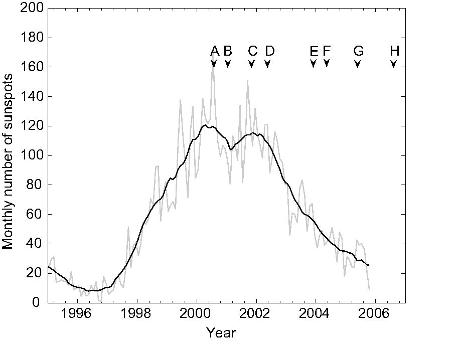
Figure 9: Chandra comet observations during the descending phase of solar cycle # 23. Monthly sunspot numbers (grey line) and smoothed monthly sunspot number (black lines) from the Solar Influences Data Analysis Center of the Department of Solar Physics, Royal Observatory of Belgium (http://sidc.oma.be/). Letters refer to the chronological order of observation.

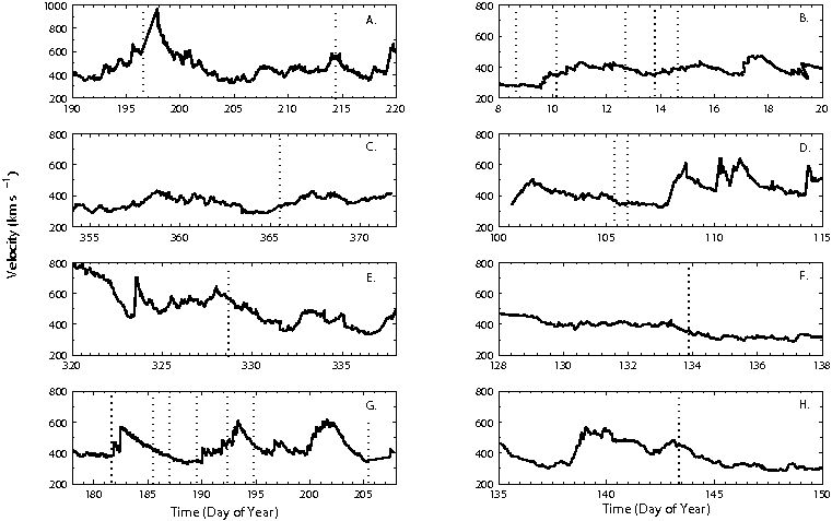
Figure 10: Solar wind proton velocities estimated from ace and soho data. For all comets, the time of the observations is indicated with a dotted line. Letters refer to the chronological order of observation.

Our survey spans the whole period between solar maximum (mid 2000) and solar minimum (mid 2006), see Fig. 9. During solar minimum, the solar wind can be classified in polar- and equatorial streams, where the polar can be found at latitudes larger than 30^∘ and the equatorial wind within 15^∘ of the helioequator. Polar streams are fast (ca. 700 km s^-1) and show only small variations in time, in contrast to the irregular equatorial wind. Cold, fast wind is also ejected from coronal holes around the equator, and when these streams interact with the slower background wind corotating interaction regions (cirs) are formed. As was illustrated by Schwadron and Cravens (2000), different wind types vary greatly in their compositions, with the cooler, fast wind consisting of on average lower charged ions than the hotter equatorial wind. This clear distinction disappears during solar maximum, when at all latitudes the equatorial type of wind dominates. In addition, coronal mass ejections are far more common around solar maximum.

There is a strong variability of heavy ion densities due to variations in the solar source regions and dynamic changes in the solar wind itself Zurbuchen & Richardson (2006). The variations mainly concern the charge state of the wind as elemental variations are only on the order of a factor of 2 (Von Steiger et al. (2000), and references therein).

We obtained solar wind data from the online data archives of ace (proton velocities and densities from the swepam instrument, heavy ion fluxes from the swics and swims instruments) and soho (proton fluxes from the Proton Monitor Instrument). Both ace and soho are located near Earth, at its Lagrangian point L1. In order to map the solar wind from L1 to the position of the comets, we used the time shift procedure described by Neugebauer et al. (2000). The calculations are based on the comet ephemeris, the location of L1 and the measured wind speed. With this procedure, the time delay between an element of the corotating solar wind arriving at L1 and the comet can be predicted. A disadvantage of this procedure is that it cannot account for latitudinal structures in the wind or the magnetohydrodynamical behavior of the wind (i.e., the propagation of shocks and cmes). These shortcomings imply that especially for comets that have large longitudinal, latitudinal and/or radial separations from Earth, the solar wind data is at best an estimate of the local wind conditions. The resulting proton velocities at the comets near the time of the Chandra observations are shown in Fig. 10.

Parallel to this helioradial and heliolongitudinal mapping, we compared our comet survey to a 3D mhd time–dependent solar wind model that was employed during most of Solar Cycle 23 (1997 - 2006) on a continuous basis when significant solar flares were observed. The model (reported by Fry et al. (2003); McKenna-Lawlor et al. (2006) and Z.K. Smith, private communication, for, respectively, the ascending, maximum, and descending phases) treats solar flare observations and maps the progress of interplanetary shocks and cmes. The papers mentioned above provide an rms error for ”hits” of $\pm 11$ hours Smith et al. (2000); McKenna-Lawlor et al. (2006). cir fast forward shocks were also taken into account in order to differentiate between the co-rotating ”quiet” and transient structures. It was important, in this differentiating analysis, to examine (as we have done here) the ecliptic plane plots of both of these structures as simulated by the deforming interplanetary magnetic field lines (see, for example, Lisse et al. (2005, 2007) for several of the comets discussed here.) Therefore, the various comet locations (Table 3) were used to estimate the probability of their X-ray emission during the observations being influenced by either of these heliospheric situations.

4.2 X-ray Observations

After its launch in 1999, 8 comets have been observed with the Chandra X-ray Observatory and Advanced ccd Imaging Spectrometer (acis). Here, we have mainly considered observations made with the acis-S3 chip, which has the most sensitive low energy response and for which the majority of comets were centered. The Chandra’s acis-S instrument provides moderate energy resolution ($\sigma\approx$ 50 eV) in the 300 to 1500 eV energy range, the primary range for the relatively soft cometary emission. All comets in our sample were re-mapped into comet-centered coordinates using the standard Chandra Interactive Analysis of Observations (ciao v3.4) software ‘sso_freeze’ algorithm.

Comet source spectra were extracted from the S3 chip with a circular aperture with a diameter of 7.5$\arcmin$, centered on the cometary emission. The exception was comet C/2001 Q4, which filled the chip and a 50% larger aperture was used. acis’ response matrices were used to model the instrument’s effective area and energy dependent sensitivity matrices were created for each comet separately using the standard ciao tools.

Due to the large extent of cometary X-ray emission, and Chandra’s relatively narrow field of view, it is not trivial to obtain a background uncontaminated by the comet and sufficiently close in time and viewing direction. We extracted background spectra using several techniques: spectra from the S3 chip in an outer region generally $>8\arcmin$, an available acis S3 blank sky observation, and backgrounds extracted from the S1 ccd. For several comets there are still a significant number of cometary counts in the outer region of the S3 ccd. Background spectra taken from the S1 chip have the advantage of having been taken simultaneous with the S3 observation and thus having the same space environment as the S3 observation. In general the background spectra were extracted with the same 7.5$\arcmin$ aperture as the source spectra but centered on the S1 chip. For comet Encke, where the S1 chip was off during the observation the background from the outer region of the S3 chip was used. Comet C/2000 WM1 (linear) was observed with the Low-Energy Transmission Grating (letg) and acis-S array. For the latter, we analyzed the zero-th order spectrum, and used a background extracted from the outer region of the S3 chip. It is possible that the proportion of incident X-rays diffracted onto the S3 chip will vary with photon energy. Background-subtracted spectra generally have a signal-to-noise at 561 eV of at least 10, and over 50 for 153P/2002 C1 (Ikeya–Zhang).

5 Spectroscopy

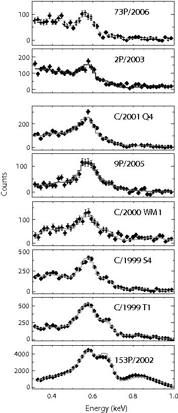
Figure 11: Observed spectrum and fit of all 8 comets observed with Chandra, grouped by their spectral shape (see text). The histogram lines indicate the CXE model fit.

The observed spectra are shown in Figure 11. The spectra suggest a classification based upon three competing emission features, i.e. the combined carbon and nitrogen emission (below 500 eV), O vii emission around 565 eV and O viii emission at 654 eV. Firstly, the C+N emission ($<$500 eV) seems to be anti-correlated with the oxygen emission. This clearly sets the spectra of 73P/2006 S.–W.3B and 2P/2003 (Encke) apart, as for those two comets the C+N features are roughly as strong as the O vii emission. In the spectra of the remaining five comets, oxygen emission dominates over the carbon and nitrogen emission below 500 eV. The O viii/O vii ratio can be seen to increase continuously, culminating in the spectrum of 153P/2002 (Ikeya–Zhang) where the spectrum is completely dominated by oxygen emission with almost comparable O viii and O vii emission features. From our modelling, we expect that the separate classes reflect different states of the solar wind, which imply different ionic abundances. To explore the obtained spectra more quantitatively, we will use a spectral fitting technique based on our cxe model to extract X-ray line fluxes.

5.1 Spectral Fitting

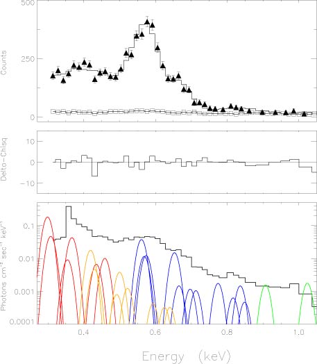
Figure 12: Details of the cxe fit for the spectrum of comet 1999/S4 (linear). Top panel: Comet (filled triangles) and background (open squares) spectrum. Middle panel: Residuals of cxe fit Bottom panel: cxe model and observed spectrum indicating the different lines and their strengths. Carbon - red; nitrogen - orange; oxygen - blue; neon - green. The unfolded model is scaled above the emission lines for the ease of presentation.

The charge exchange mechanism implies that cometary X-ray spectra result from a set of solar wind ions, which produce at least 35 emission lines in the regime visible with Chandra. As comets are extended sources, these lines cannot all be resolved. All spectra were therefore fit using the 6 groups of fixed lines of our cxe model (see Table 2) and spectral parameters were derived using the least squares fitting procedure with the xspec package. The relative strengths from all lines were fixed per ionic species, according to their velocity dependent emission cross sections. Thus, the free parameters were the relative fluxes of the C, N and O ions contained in our model.

Two additional Ne lines at 907 eV (Ne ix) and 1024 eV (Ne x) were also included, giving a total of 8 free parameters. All line widths were fixed at the acis-S3 instrument resolution.

The spectra were fit in the 300 to 1000 eV range. This provided 49 spectral bins, and thus 41 degrees of freedom. acis spectra below 300 eV are discarded because of the rising background contributions, calibration problems and a decreased effective area near the instrument’s carbon edge.

As a more detailed example of the cxe model and comparison to the data, we show in Fig 12 the acis-S3 data for C/1999 S4 (linear). The figure shows the background subtracted source spectrum over-plotted with the background spectrum, the difference between the model and data, and the model spectrum and data to indicate to contribution of the different ions. Only the emission lines with $>$3% strength of the strongest line in their species are shown for ease of presentation.

The fluxes obtained by our fitting are converted into relative ionic abundances by weighting them by their velocity dependent emission cross sections. For comets observed near the ecliptic plane ($<15^{\circ}$), solar wind conditions mapped to the comet were used (Section 4.1). For comets observed at higher latitudes, these data are most likely not applicable and a solar wind velocity of 500 km s^-1 was assumed.

Table 4: Results of the cxe-model fit for all cometary spectra. Fluxes are given in dimensions of 10^-5 photons cm^-2 s^-1. Errors are obtained by averaging over the calculated + and - 90$\%$ confidence contours and averaged those (corresponding to $\chi^{2}=2.7$ or $1.6\leavevmode\nobreak\ \sigma$)

Ion	Line	C/1999 S4			C/1999 T1			C/2000 WM1			153P /2002			2P/2003			C/2001 Q4			9P/2005			73P/2006
	(eV)	(linear)			(McNaught–Hartley)			(linear)			(Ikeya–Zhang)			(Encke)			(neat)			(Tempel 1)			(SW3–B)
O viii	653	23	$\pm$	2.0	25	$\pm$	1.6	20	$\pm$	3.9	357	$\pm$	14	1.95	$\pm$	0.36	9.7	$\pm$	1.7	3.5	$\pm$	0.98	1.5	$\pm$	0.57
O vii	561	57	$\pm$	3.4	47	$\pm$	2.7	52	$\pm$	7.1	296	$\pm$	1.0	7.12	$\pm$	0.84	52	$\pm$	4.3	16	$\pm$	1.6	11	$\pm$	1.3
C vi	368	65	$\pm$	17	36	$\pm$	15	85	$\pm$	40	288	$\pm$	1.8	18	$\pm$	7.0	47	$\pm$	36	0.5	$\pm$	7.0	21	$\pm$	10
C v	299	276	$\pm$	85	278	$\pm$	90	62	$\pm$	193	1052	$\pm$	18	192	$\pm$	62	809	$\pm$	280	121	$\pm$	89	326	$\pm$	109
N vii	500	5.2	$\pm$	4.7	11	$\pm$	3.6	9.8	$\pm$	9.2	98	$\pm$	1.6	1.3	$\pm$	1.2	17	$\pm$	6.4	0	$\pm$	0.98	0.1	$\pm$	1.25
N vi	420	27	$\pm$	8.5	17	$\pm$	6.9	19	$\pm$	19	123	$\pm$	0.84	4.8	$\pm$	3.3	36	$\pm$	16	7.6	$\pm$	5.0	13.0	$\pm$	6.0
Ne ix	907	2.4	$\pm$	1.1	1.97	$\pm$	0.67	6.7	$\pm$	1.7	38	$\pm$	0.11	0.68	$\pm$	0.2	1.4	$\pm$	0.54	0	$\pm$	0.17	0.48	$\pm$	0.24
Ne x	1024	2.7	$\pm$	1.2	0.41	$\pm$	0.47	4.6	$\pm$	2.1	8.2	$\pm$	0.02	0.72	$\pm$	0.24	0.8	$\pm$	0.46	0.07	$\pm$	0.22	0.02	$\pm$	0.25
$\chi^{2}_{R}$		1.4			1.1			1.4			1.7			1.4			1.4			0.91			1

Table 5: Solar wind abundances relative to O⁷⁺, obtained from the cxe-model fit.

Ion	C/1999 S4			C/1999 T1			C/2000 WM1			153P /2002			2P/2003			C/2001 Q4			9P/2005			73P/2006
	(linear)			(McNaught–Hartley)			(linear)			(Ikeya–Zhang)			(Encke)			(neat)			(Tempel 1)			(SW3–B)
O8+	0.32	$\pm$	0.03	0.42	$\pm$	0.04	0.31	$\pm$	0.07	0.96	$\pm$	0.04	0.19	$\pm$	0.04	0.17	$\pm$	0.03	0.19	$\pm$	0.06	0.10	$\pm$	0.04
C6+	1.4	$\pm$	0.4	0.95	$\pm$	0.4	2.0	$\pm$	1.0	1.21	$\pm$	0.0	2.9	$\pm$	1.1	1.2	$\pm$	0.9	0.0	$\pm$	0.6	2.3	$\pm$	1.1
C5+	12	$\pm$	3.8	15	$\pm$	4.8	3.0	$\pm$	9.3	8.9	$\pm$	0.2	56	$\pm$	19.3	49	$\pm$	17.4	22	$\pm$	15.9	71	$\pm$	24.9
N7+	0.07	$\pm$	0.06	0.19	$\pm$	0.06	0.14	$\pm$	0.14	0.25	$\pm$	0.00	0.14	$\pm$	0.13	0.25	$\pm$	0.10	0.00	$\pm$	0.05	0.008	$\pm$	0.08
N6+	0.63	$\pm$	0.21	0.47	$\pm$	0.20	0.49	$\pm$	0.49	0.56	$\pm$	0.00	0.79	$\pm$	0.55	1.1	$\pm$	0.52	0.72	$\pm$	0.48	1.5	$\pm$	0.72
Ne10+	0.02	$\pm$	0.01	0.004	$\pm$	0.005	0.044	$\pm$	0.02	0.01	$\pm$	0.0001	0.05	$\pm$	0.02	0.008	$\pm$	0.004	0.002	$\pm$	0.007	0.001	$\pm$	0.01

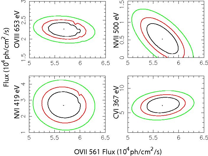
Figure 13: Parameter sensitivity for the major emission features in the fit of C/1999 S4 (linear), with respect to the O vii 561 eV feature. All units are 10^-4 photons cm^-2 s^-1. The contours indicate a $\chi_{R}^{2}$ of 9.2 (or 99$\%$ confidence, largest, green contour), a $\chi_{R}^{2}$ of 4.6 (90$\%$, red contour) and a $\chi_{R}^{2}$ of 2.3 (68$\%$, smallest, blue contour).

5.2 Spectroscopic Results

Table 6: Solar wind abundance relative to O⁷⁺, obtained for comet linear S4. References: Bei ’03 – Beiersdorfer et al. (2003), Kra ’04 – Krasnopolsky (2004), Kra ’06 – Krasnopolsky (2006), Otr ’06 – Otranto et al (2006) and S&C ’00 – Schwadron and Cravens (2000). Dots indicate that an ion was included in the fitting, but no abundances were derived; dash means that an ion was not included in the fitting. Otranto et al (2006) did not fit the observed spectrum, but used a combination of ace-data and solar wind averages from Schwadron and Cravens (2000) to compute a syntectic spectrum of the comet. Solar wind averages are given for comparison Schwadron and Cravens (2000)

Ion	this work			Bei 03			Kra 04			Kra 06			Otr 06
O8+	0.32	$\pm$	0.03	0.13	$\pm$	0.03	0.13	$\pm$	0.05	0.15	$\pm$	0.03	0.35	0.35
C6+	1.4	$\pm$	0.4	0.9	$\pm$	0.3	0.7	$\pm$	0.2	0.7	$\pm$	0.2	1.02	1.59
C5+	12	$\pm$	4.0	11	$\pm$	9	…			1.7	$\pm$	0.7	1.05	1.05
N7+	0.07	$\pm$	0.06	0.06	$\pm$	0.02	–			–			0.03	0.03
N6+	0.63	$\pm$	0.21	0.5	$\pm$	0.3	–			–			0.29	0.29
Ne10+	0.02	$\pm$	0.01	–			–			–			–	–
Ne9+	…			–			$(15\pm 6)\times 10^{-3}$			$(20\pm 7)\times 10^{-3}$			–	–

The fits to all cometary spectra are shown in Fig. 11 and the results of the fits are given in Table 5. For the majority of the comets, the model is a good fit to the data within a 95% confidence limit ($\chi_{R}^{2}\approx 1.4$). Results for comet 153P/2002 (Ikeya–Zhang) are presented in Table 5 with an additional systematic error to account for its brightness and any uncertainties in the response.

The spectra for all comets are well reproduced in the 300 to 1000 eV range. The nitrogen contribution is statistically significant for all comets except the fainter ones, 2P/2003 (Encke) and 73P/2006 (S.-W.3B). For example, removing the nitrogen components from linear S4’s cxe model and re-fitting, increases $\chi^{2}_{R}$ to over 7.

$\chi^{2}$ contours for C/1999 S4 (linear) are presented in Fig 13. The line strengths for each ionic species are generally well constrained, except where spectral features overlap. This can be readily seen when comparing the contours for the N vii 500 eV and O vii 561 eV features where a strong anti-correlation exists (Figure 12). Due to the limited resolution of acis an increase in the N vii feature will decrease the O vii strength. Similar anti-correlations exist between the nitrogen N vi or N vii and C v 299 eV lines. Since the line strength for the main line in each ionic species is linked to weaker lines, a range of energies can contribute and better constrain its strength. However with O vii as the strongest spectral feature the nitrogen and carbon components may be artificially lower as a result of the aforementioned anti-correlations. The lack of effective area due to the carbon edge in the acis response also may over-estimate the C v line flux. The neon features were well constrained for the brighter comets, but this is a region of lower signal and some caution must be taken when treating the neon line strengths and they are included here largely for completeness.

In the case of 153P/Ikeya–Zhang, the $\chi^{2}_{R}>1.4$. The main discrepancy is that the model produces not enough flux in the 700 to 850 eV range compared to the observed spectrum. This may reflect an underestimation of higher O viii transitions or the presence of species not (yet) included in the model, such as Fe. This will be discussed further in the last section of this paper and in a separate paper dedicated to the observations of this comet (K. Dennerl, private communication).

One of the best studied comets is C/1999 S4 (linear), because of its good signal-to-noise ratio. To discuss our results, we will compare our findings with earlier studies of this comet. In general, the spectra analyzed here have more counts than earlier analyzes, because of improvements in the Chandra processing software and because we took special care to use a background that is as comet-free as possible. Previous studies appear to have removed true comet signal when the background subtraction was performed. In particular, both the Krasnopolsky (2004) and Lisse et al. (2001) studies used background regions from the outer part of the S3 chip and this may have still had true cometary emission. Krasnopolsky (2004) subtracted over 70% of the total signal as background. We find that using the S1-chip, the background contributes only 20% of the total counts.

Different attempts to derive relative ionic abundances from C1999/S4’s X-ray spectrum are compared in Table 6. Our atomic physics based spectral analysis combines the benefits of earlier analytical approaches by Kharchenko and Dalgarno (2000, 2001); Beiersdorfer et al. (2003). These methods were all applied to just one or two comets. Beiersdorfer et al. (2003) interpret C1999/S4’s X-ray spectrum by fitting it with 6 experimental spectra obtained with their ebit setup. The resulting abundances are very similar to ours. The advantage of their method is that it includes multiple electron capture, but in order to observe the forbidden line emission, the spectra were obtained with trapped ions colliding at CO₂, at collision energies of 200 to 300 eV or ca. 30 km s^-1. As was shown in Fig. 3, the cxe hardness ratio may change rapidly below 300 km s^-1, implying an overestimation of the higher order lines compared to the $n=2\to 1$ transition, which for O vii overlap with the O viii emission. We therefore find higher abundances of O⁸⁺.

Krasnopolsky (2004, 2006) obtained fluxes and ionic abundances by fitting the spectrum with 10 lines of which the energies were semi-free. Their analysis thus does not take the contamination of unresolved emission into account, and N vi and N vii are not included in the fit. The line energies were attributed to cxe lines of mainly solar wind C and O but also to ions of Mg and Ne. The inclusion of the resulting low energy emission (near 300 eV) results in lower C⁵⁺ fluxes (see also Otranto et al (2006)).

There are several factors that may contribute to the unexpectedly low C vi/C v ratios: 1) There may be a small contribution to the C v line from other ions in the 250-300 eV range (e.g. Si, Mg, Ne) that are currently not included in the model. Including these species in the model would lower the C v flux, but probably only with a small amount. 2) The low acis effective area in the 250-300 eV region allows the C v flux to be unconstrained, and this increases the uncertainty in the C v flux. We estimate that the uncertainty in the effective area, introduced by the carbon edge, can account for an uncertainty as large as a factor of 10 in the observed C v/C vi ratios.

We will not compare our results with measured ace/swics ionic data. As discussed in section 4, the solar wind is highly variable in time and its composition can change dramatically over the course of less than a day. Variations in the solar wind’s ionic composition are often more than 50% during the course of an observation. Data on N, Ne, and O⁸⁺ ions have not been well documented as the errors of these abundances are dominated by counting statistics. As discussed above, latitudinal and corotational separations imply large inaccuracies in any solar wind mapping procedure. These conditions clearly disfavor modelling based on either average solar wind data or ace/swics data.

6 Comparative Results

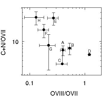
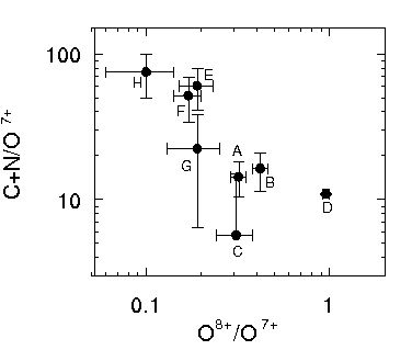
Figure 14: Flux ratios of all observed comets. The low energy C+N feature is anti-correlated to the oxygen ionic ratio. Letters refer to the chronological order of observation.

Figure 15: Ion ratios of all observed comets. The C+N ionic abundantie is anti-correlated to the oxygen ionic ratio. Letters refer to the chronological order of observation.

Table 7: Correlation between classification according to spectral shape and comet/solar wind characteristics during the observations. Comet families from Marsden & Williams (2005). Phase refers to where in the solar cycle the comet was observed, where 1 is the solar maximum and 0 the solar minimum of cycle #23’s descending phase. For other references, see Table 3.

Class	#	Comet	Comet	Q	Latitude	Wind Type
			Family	(1028 mol. s-1)
cold	H	73P/2006 (S.-W.3B)	Jupiter	2	0.5	cir
	E	2P/2003 (Encke)	Jupiter	0.7	11.4	Flare/PS
warm	F	C/2001 Q4 (neat)	unknown	10	-3	Quiet
	G	9P/2005 (Tempel 1)	Jupiter	0.9	0.8	Quiet
hot	C	C/2000 WM1 (linear)	unknown	3-9	-34	PS
	A	C/1999 S4 (linear)	unknown	3	24	icme
	B	C/1999 T1 (McNaught–Hartley)	unknown	6-20	15	Flare/cir
	D	C/2002 C1 (Ikeya–Zhang)	Oort	20	26	icme

As noted in Section 5, spectral differences show up in the behavior of the low energy C+N emission ($<$ 500 eV), the O vii emission at 561 eV and the O viii emission at 653 eV. Figure 15 shows a color plot of the fluxes of these three emission features, and Figure 15 the corresponding ionic abundances. There is a clear separation between the two comets with a large C+N contribution and the other ‘oxygen-dominated’ comets, which on their turn show a gradual increase in the oxygen ionic ratio. This sample of comet observations suggest that we can distinguish two or three spectral classes.

Table 7 surveys the comet parameters for the different spectral classes. The outgassing rate, heliocentric- or geocentric distance and comet family do not correlate to the different classes, in accordance with our model findings. The data does suggest a correlation between latitude and wind conditions during the observations. At first sight, the apparent correlation between latitude and oxygen ratio seems paradoxical. According to the bimodal structure of the solar wind the fast, cold wind dominates at latitudes $>15^{\circ}$, implying less O viii emission. In Figure 9, the comet observations are shown with respect to the phase of the last solar cycle. Interestingly, we note that all comets that were observed at higher latitudes were observed around solar maximum. The solar wind is highly chaotic during solar maximum and the frequency of impulsive events like CMEs is much higher than during the descending and minimum phase of the cycle. This explains both why the comets observed in the period 2000–2002 encountered a disturbed solar wind and why our survey does not contain a sample of the cool fast wind from polar coronal holes.

The observed classification can therefore be fully ascribed to solar wind states. The first class is associated with cold, fast winds with lower average ionization. These winds are found in cirs and behind flare related shocks. The spectra due to these winds are dominated by the low energy x-rays, because of the low abundances of highly charged oxygen. At the relevant temperatures, most of the solar wind oxygen is He-like O⁶⁺, which does not produce any emission visible in the 300–1000 eV regime accessible with Chandra. Secondly, there is an intermediate class with two comets that were all observed during periods of quiet solar wind. These comets interacted with the equatorial, warm slow wind. The third class then comprises comets that interacted with a fast, hot, disturbed wind associated with icmes or flares. From the solar wind data, Ikeya–Zhang was probably the most extreme example of this case. This comet had 10 times more signal than any other comet in our sample and small discrepancies in the response may be important at this level. Extending into the 1-2 keV regime, a preliminary analysis indicates the presence of bare and H-like Si, Mg and Fe xv-xx ions, in accordance with ace measurements of icme compositions Lepri & Zurbuchen (2004).

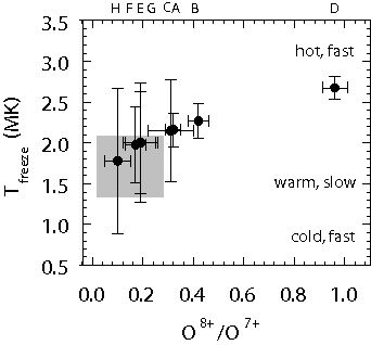
Figure 16: Spectrum derived ionic oxygen ratios and corresponding freezing-in temperatures from Mazotta et al. (1998). The shaded area indicates the typical range of slow wind associated with streamers. Letters refer to the chronological order of observation.

The variability and complex nature of the solar wind allows for many intermediate states in between these three categories Zurbuchen et al. (2002), which explain the gradual increase of the O viii/O vii ratio that we observed in the cometary spectra. As the solar wind is a collisionless plasma, the charge state distribution in the solar wind is linked to the temperature in its source region. Ionic temperatures are therefore a good indicator of the state of the wind encountered by a comet. The ratio between O⁷⁺ and O⁶⁺ ionic abundances has been demonstrated to be a good probe of solar wind states. Zurbuchen et al. (2002) observed that slow, warm wind associated with streamers typically lies within $0.1<$ O⁷⁺/O⁶⁺ $<1.0$, corresponding to freezing in temperatures of 1.3–2.1 MK. The corresponding temperature range is indicated in the Figure 16. In the figure, we show the observed O⁸⁺ to O⁷⁺ ratios and the corresponding freezing-in temperatures from the ionizational/recombination equilibrium model by Mazotta et al. (1998). Most observations are within or near to the streamer-associated range of oxygen freezing in temperatures. Four comets interacted with a wind significantly hotter than typical streamer winds, and in all four cases we found evidence in solar wind archives that the comets most likely encountered a disturbed wind.

7 Conclusions

Cometary X-ray emission arises from collisions between bare- and H-like ions (such as C, N, O, Ne, …) with mainly water and its dissociation products OH, O and H. The manifold of dependencies of the cxe mechanism on characteristics of both comet and wind offers many diagnostic opportunities, which are explored in the first part of this paper. Charge exchange cross sections are strongly dependent on the velocity of the solar wind, and these effects are strongest at velocities below the regular wind conditions. This dependency might be used as a remote plasma diagnostics in future observations. Ruling out collisional opacity effects, we used our model to demonstrate that the spectral shape of cometary cxe emission is in the first place determined by local solar wind conditions. Cometary X-ray spectra hence reflect the state of the solar wind.

Based on atomic physic modelling of cometary charge exchange emission, we developed an analytical method to study cometary X-ray spectra. First, the data of 8 comets observed with Chandra were carefully reprocessed to avoid the subtraction of cometary signal as background. The spectra were then fit using an extensive data set of velocity dependent emission cross sections for eight different solar wind species. Although the limited observational resolution currently available hampers the interpretation of cometary X-ray spectra to some degree, our spectral analysis allows for the unravelling of cometary X-ray spectra and allowed us to derive relative solar wind abundances from the spectra.

Because the solar wind is a collisionless plasma, local ionic charge states reflect conditions of its source regions. Comparing the fluxes of the C+N emission below 500 eV, the O vii emission and the O viii emission yields a quantitative probe of the state of the wind. In accordance with our modelling, we found that spectral differences amongst the comets in our survey could be very well understood in terms of solar wind conditions. We are able to distinguish interactions with three different wind types, being the cold, fast wind (I), the warm, slow wind (II); and the hot, fast, disturbed wind (III). Based on our findings, we predict the existence of even cooler cometary X-ray spectra when a comet interacts with the fast, cool high latitude wind from polar coronal holes. The upcoming solar minimum offers the perfect opportunity for such an observation.

Appendix A Observations within this Survey

This Appendix presents the observational details of the Chandra data and the corresponding solar wind state. The prefix ’FF’ (fearless forecast) used in this appendix refers to the real time forecasting of coronal mass ejection shocks arrivals at Earth. The numbers were so-named for flare/coronal shock events during solar cycle #23.

A.1 C/1999 S4 (linear)

X-rays. The first Chandra cometary observation was of comet C/1999 S4 (linear) Lisse et al. (2001), with observations being made both before and after the breakup of the nucleus. Due to the low signal-to-noise ratio of the second detection, only the July 14th 2000 pre-breakup observation is discussed here. Summing the 8 pointings of the satellite gave a total time interval of 9390 s. In this period, the acis-S3 ccd collected a total of 11 710 photons were detected in the range 300–1000 eV. Detections out side this range or on other acis-ccds were not attributed to the comet. As a result, data from the S1-ccd (which is configured identically to S3) may be used as an indicator of the local X-ray background.

The morphology can be described by a crescent shape, with the maximum brightness point 24 000 km from the nucleus on the Sun-facing side. The brightness dims to 10% of the maximum level at 110 000 km from the nucleus.

Solar wind. A large velocity jump can be seen around DoY 199, which was due to the famous ”Bastille Day” flare on 14 July (FF#153, Dryer et al (2001); Fry et al. (2003)). This flare reached the comet only after the first observation. At July 12, 2017UT a solar flare started at N17W65 (FF#152), which was nicely placed to hit this comet with a very high probability during the first observations Fry et al. (2003). As for the second observation, there was another flare on July 28, S17E24, at 1713 UT (FF#164) and there was a high probability that its shock’s weaker flank hit the comet.

A.2 C/1999 T1 (McNaught–Hartley)

X-rays. The allocated observing time of comet McNaught–Hartley was partitioned into 5 one-hour-slots between January 8th and January 15th, 2001 Krasnopolsky et al. (2002). The strongest observing period was on January 8th, when $\Delta=1.37$ AU and $r_{h}=1.26$ AU.

There were 15 000 total counts observed by the acis-S3 ccd between 300 and 1000 eV. The emission region can be described by a crescent, with the peak brightness is at 29 000 km from the nucleus. The brightness dims to 10% of the maximum at a cometocentric distance of 260 000 km. Again, the acis-S1 ccd may be used to indicate the local background signal.

Solar wind. The comet was not within the heliospheric current/plasma sheet (HCS/HPS). Two corotating cirs are probably associated with the first two observations. Two flares (FF#233 and #234) took place; however, another corotating cir more likely arrived before the flare’s transient shock’s effects did McKenna-Lawlor et al. (2006).

A.3 C/2000 WM1 (linear)

X-rays. The only attempt to use the high-resolution grating capability of the acis-S array was made with comet C/2000 WM1 (linear). Here, the Low-Energy Transmission Grating (letg) was used. The dimness of the observed X-rays, and the extended nature of the emitting atmosphere meant that the grated spectra did not yield significant results. It is still possible to extract a spectrum based on the pulse-heights generated by each X-ray detection on the acis-S3 chip, although the morphology is not recorded. 6300 total counts were recorded for the pulse-height spectrum of the S3 chip in the 300 to 1000 eV range.

Solar wind. Comet WM1 was observed at the highest latitude available within this survey, and at a latitude of 34 degrees, it was far outside the hcs. During the observations, this comet might have experienced the southerly flank of the shock of a strong X3.4 flare at S20E97 and its icme and shock on December 28, 2001 (FF#359) McKenna-Lawlor et al. (2006).

A.4 153P/2002 (Ikeya–Zhang)

X-rays. The brightest X-ray comet in the Chandra archive is 153P/2002 (Ikeya–Zhang). The heliographic latitude, geocentric distance and heliocentric distance were comparable to those for comet C/1999 S4 (linear), with a latitude of $26^{\circ}$, $\Delta=0.457$ AU and $r_{h}=0.8$ AU. Rather than periodically re-point the detector to track the comet, the pointing direction was fixed and the comet was monitored as it passed through the field of view, thus increasing the effective FoV. There were two observing periods on April 15th 2002, each lasting for approximately 3 hours and 15 minutes. In both periods, a strong cometary signal is detected on all of the activated acis-ccds. Consequently, a background signal cannot be taken from the observation. A crescent shape on the Sun side of the comet is observed over all of the ccd array. Over 200 000 total counts were observed from the S3 chip in the 300 to 1000 eV range. The time intervals for each observing period are 11 570 and 11 813 seconds.

Solar wind. Like C/2000 WM1, this comet was observed at a relatively high heliographic latitude. Solar wind data obtained in the ecliptic plane can therefore not be used to determine the wind state at the comet. 153P/2002 (Ikeya–Zhang) was well-positioned during the first observation on 15 April 2002 for a flare at N16E05 (FF#388) on 12 April 2002. During the second observation on 16 April, there was an earlier flare on 14 April at N14W57, but this flare was probably too far to the west to be effective McKenna-Lawlor et al. (2006). The comet was observed at a high latitude, and hence ace solar wind data is most likely not applicable.

A.5 2P/2003 (Encke)

X-rays. The Chandra observation of Encke took place on the 24th of November 2003 Lisse et al. (2005), when the comet had a heliocentric distance of $r_{h}=0.891$ AU and a geocentric distance of $\Delta=0.275$ AU and a heliographic latitude of 11.4 degrees. The comet was continuously tracked for over 15 hours, resulting in a useful exposure of 44 000 seconds. The acis-S3 ccd counted 6140 X-rays in the range 300–1000 eV.

The brightest point was offset from the nucleus by 11 000 km, dimming to 10% of this value at a distance of 60 000 km.

The acis-S1 ccd was not activated in this observation. The low quantum efficiency of the other activated ccds below 0.5 keV makes them unsuitable as background references.

Solar wind. The proton velocity decreased during observations from 600 km s^-1 to 500 km s^-1. A flare on 20 November 2003, at N01W08 (FF#525), was well-positioned to affect the observations on 23 November (data from work in progress by Z.K. Smith et al.). The comet most likely interacted with the overexpanded, rarified plasma flow that followed the earlier hot shocked and compressed flow behind the flare’s shock.

A.6 C/2001 Q4 (neat)

X-rays. A short observation of comet C/2001 Q4 was made on May 12 2004, when the geocentric and heliocentric distances were $\Delta=0.362$ AU and $r_{h}=0.964$ AU respectively. With a heliographic latitude of 3 degrees, the comet was almost in the ecliptic plane. From 3 pointings, the useful exposure was 10 328 seconds. The acis-S3 chip detected 6540 X-rays in between 300 and 1000 eV. The acis-S1 was used as a background signal.

Solar wind. There was no significant solar activity during the observations (Z.K. Smith et al., ibid.). From solar wind data, the comet interacted with a quiet, slow 352 km s^-1 wind.

A.7 9P/2005 (Tempel 1)

X-rays. The observation of comet 9P/2005 (Tempel 1) was designed to coincide with the Deep Impact mission Lisse et al. (2007). The allocated observation time of 291.6 ks was split into 7 periods, starting on June 30th, July 4th (encompassing the Deep Impact collision), July 5th, July 8th, July 10th, July 13th and July 24th. The brightest observing periods were June 30th and July 8th. The focus here is on the June 30th observation. On this date, $r_{h}=1.507$ AU and $\Delta=0.872$ AU.

The useful exposure was 50 059 seconds, with a total of 7300 counts, 4000 from the June 30th flare alone, were detected in the energy range of 300–1000 eV.

The brightest point for the June 30th observation was located 11 000 km from the nucleus. The morphology appears to be more spherical than in other comet observations.

Solar wind. Observations were taken over a long time span covering different solar wind environments. There was no significant solar activity during the 30 June 2005 observations (Z.K. Smith et al., ibid. Lisse et al. (2007)). From the ace data, it can be seen that at June 30, the comet most likely interacted with a quiet, slow solar wind.

A.8 73P/2006 (Schwassmann–Wachmann 3B)

X-rays. The close approach of comet 73P/2006 (Schwassmann–Wachmann 3B) in May 2005 ($\Delta=0.106$ AU, $r_{h}=0.965$ AU) provided an opportunity to examine cometary X-rays in high spatial resolution. Chandra was one of several X-ray missions to focus on one of the large fragments of the comet. Between 300 and 1000 eV, 6285 counts were obtained in a useful exposure of 20 600 seconds.

Solar wind. There was a weak flare on 22 May 2006 (FF#655, Z.K. Smith, priv. comm.). A sequence of three high speed coronal hole streams passed the comet in the period around the observations and a corotating cir might have reached the comet in association with the observations on 23 May, which is confirmed by the mapped solar wind data.