Burgers Turbulence

Abstract

The last decades witnessed a renewal of interest in the Burgers equation. Much activities focused on extensions of the original one-dimensional pressureless model introduced in the thirties by the Dutch scientist J.M. Burgers, and more precisely on the problem of Burgers turbulence, that is the study of the solutions to the one- or multi-dimensional Burgers equation with random initial conditions or random forcing. Such work was frequently motivated by new emerging applications of Burgers model to statistical physics, cosmology, and fluid dynamics. Also Burgers turbulence appeared as one of the simplest instances of a nonlinear system out of equilibrium. The study of random Lagrangian systems, of stochastic partial differential equations and their invariant measures, the theory of dynamical systems, the applications of field theory to the understanding of dissipative anomalies and of multiscaling in hydrodynamic turbulence have benefited significantly from progress in Burgers turbulence. The aim of this review is to give a unified view of selected work stemming from these rather diverse disciplines.

1 From interface dynamics to cosmology

At the end of the thirties, the Dutch scientist J.M. Burgers [26] introduced a one-dimensional model for pressure-less gas dynamics. He was hoping that the use of a simple model having much in common with the Navier–Stokes equation would significantly contribute to the study of fluid turbulence. This model now known as the Burgers equation

$$\partial_{t}v+v\,\partial_{x}v=\nu\,\partial_{x}^{2}v,$$ (1.1)

has not only the same type of hydrodynamical (or advective) quadratic nonlinearity as the Navier–Stokes equation that is balanced by a diffusive term, but it also has similar invariances and conservation laws (invariance under translations in space and time, parity invariance, conservation of energy and momentum in one dimension for $\nu=0$).

Such hopes appeared to be shattered when in the fifties, Hopf [67] and Cole [33] showed that the Burgers equation can be integrated explicitly. This model thus lacks one of the essential properties of Navier–Stokes turbulence: sensitivity to small perturbations in the initial data and thus the spontaneous arise of randomness by chaotic dynamics. Unable to cope with such a fundamental aspect, the Burgers equation then lost its interest in “explaining” fluid turbulence.

In spite of this, the Burgers equation reappeared in the eighties as the asymptotic form of various nonlinear dissipative systems. Physicists and astrophysicists then devoted important effort to the understanding of its multi-dimensional form and to the study of its random solutions arising from random initial conditions or a random forcing. The goal of this paper is to review selected works that exemplify this strong renewal of interest in Burgers turbulence.

The rest of this section is dedicated to the description of several physical situations where the Burgers equation arises. We will then see in section 2 that in any dimension and in the limit of vanishing viscosity, the solutions to the Burgers equation can be expressed in an explicit manner in the decaying case or in an implicit manner in the forced case, in terms of a variational principle that permits a systematic classification of its various singularities (shocks and others) and of their local structure (normal form). Section 3 is dedicated to the study of the decay of the solutions to the one-dimensional unforced Burgers equation with random initial data. The multi-dimensional decaying problem is discussed in section 4. The motivation comes from cosmology where large-scale structures can be described in terms of mass transport by solutions to the Burgers equation. The basic principles of the forced Burgers turbulence are discussed in section 5 where the notions of global minimizer and topological shocks are introduced. Section 6 is dedicated to the study of the solutions to the periodically kicked Burgers equation and their relation with Aubry–Mather theory for commensurate-incommensurate phase transitions. Section 7 reviews various studies of the stochastically forced Burgers equation in one dimension with a particular emphasize on questions that are arising from the statistical study of turbulent flows. Finally, section 8 encompasses concluding remarks and a non-exhaustive list of open questions on the problem of the Burgers turbulence.

1.1 The Burgers equation in statistical mechanics

The Burgers equation appears in condensed matter, in statistical physics, and also beyond physics in vehicle traffic models (see [32], for a review on this topic). When a random forcing term is added - usually a white noise in time - it is used to describe various problems of interface deposition and growth (see, for instance, [5]). An instance frequently studied is the Kardar–Parisi–Zhang (KPZ) model [74]. This continuous version of ballistic deposition models accounts for the lateral growth of the interface. Let us indeed consider an interface where particles deposit with a random flux $F$ that depends both on time $t$ and on the horizontal position ${\vec{x}}$. The growth of the local height $h$ happens in the direction normal to the interface and its time evolution is given by

$$\partial_{t}h-\frac{1}{2}\left|\nabla h\right|^{2}=\nu\nabla^{2}h+F,$$ (1.2)

where the first term of the right-hand side represents the relaxation due to a surface tension $\nu$. The gradient of (1.2) gives the multidimensional Burgers equation

$$\partial_{t}{\vec{v}}+{\vec{v}}\cdot\nabla{\vec{v}}=\nu\,\nabla^{2}{\vec{v}}-\nabla F,\qquad{\vec{v}}=-\nabla h,$$ (1.3)

forced by the random potential $F$. As we will see later, shocks generically appear in the solution to the Burgers equation in the inviscid limit $\nu\to 0$. They correspond to discontinuities of the derivative of the height $h$. The KPZ model is hence frequently used to understand the appearence of roughness in various interface problems, as for instance front propagation in randomly distributed forests (see, e.g., [101]).

The Hopf–Cole transformation ${\mathcal{Z}}=\exp(h/2\nu)$ allows rewriting (1.2) as a linear problem with random coefficients.

$$\partial_{t}{\mathcal{Z}}=\nu\,\nabla^{2}{\mathcal{Z}}+\frac{1}{2\nu}F\,{\mathcal{Z}},$$ (1.4)

This equation appears in many complex systems, as for instance directed polymers in random media [75, 22]. Indeed the solution ${\mathcal{Z}}({\vec{x}},t)$ is exactly the partition function of an elastic string in the random potential $(1/2\nu)\,F({\vec{x}},t)$, subject to the constraint that its boundary is fixed at $({\vec{x}},t)$. Note that here, the time variable $t$ is actually a space variable in the main direction of the polymer.

1.2 The adhesion model in cosmology

The multidimensional Burgers equation has important applications in cosmology where it is closely linked to what is usually referred to as the Zel’dovich approximation [112]. In the limit of vanishing viscosity $\nu\to 0$ the Burgers equation is known as the adhesion model [62]. Right after the decoupling between baryons and photons, the primitive Universe is a rarefied medium without pressure composed mainly of non-collisional dust interacting through Newtonian gravity. The initial density of this dark matter fluctuates around a mean value $\bar{\rho}$. These fluctuations are responsible for the formation of the large-scale structures in which both the dark non-baryonic matter and the luminous baryonic matter concentrate. A hydrodynamical formulation of the cosmological problem leads to a description where matter evolves with a velocity ${\vec{v}}$, solution of the Euler–Poisson equation (see, e.g., [98], for further details).

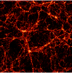
(a)

(b)

Figure 1: (a) Projection of the matter distribution in a slice obtained from an N-body simulation by the Virgo consortium [71]. (b) Composite picture showing the superposition of the results of an N-body simulation with the skeleton of the results obtained from the adhesion model (from [78]).

In the linear theory of the gravitational instability, that is for infinitesimally small initial fluctuations of the density field, an instability is obtained with potential dominant modes (i.e. ${\vec{v}}=-\nabla\Psi$) and, in the suitable coordinates, the gravitational interactions can be neglected. In 1970, Zel’dovich proposed to extend these two properties to the nonlinear régimes where density fluctuations become important. In this approximation, he also postulates that the acceleration is a Lagrangian invariant, leading to the formation of caustics. N-body simulations however show that the large-scale structures of the Universe are much simpler than caustics: they resemble sort of thin layers in which the particles tend to be trapped (see figure 1(a)).

It was shown by Gurbatov and Saichev [62] that these structures are very well approximated by those obtained when constraining the particles not to cross each other but to stick together. Even if this mechanism is not collisional but rather gravitational (probably due to instabilities at small spatial scales), its effect can be modeled by a small viscous diffusive term in the Euler–Poisson equation and thus amounts to considering the Burgers equation in the limit of vanishing viscosity.

1.3 A benchmark for hydrodynamical turbulence

As a nonlinear conservation law, and since its solution can be easily known explicitly, the one-dimensional Burgers equation frequently serves as a testing ground for numerical schemes, and especially for those dedicated to compressible hydrodynamics. For instance, it is a central example for the validation of finite-volumes schemes.

The Burgers equation was also used for testing statistical theories of turbulence. For instance, field theoretical methods have frequently been applied to turbulence (see [96, 102]). These approaches had very little impact until recently when they led to significant advances in the understanding of intermittency in passive scalar advection (see, e.g., [46] for a review). In the past such attempts were mostly based on a formal expansion of the nonlinearity using, for instance, Feynman graphs. Since the Burgers equation has the same type of quadratic nonlinearity as the Navier–Stokes equation, such methods are applicable in both instances. From this point of view, it is important to know answers for Burgers turbulence to questions that are generally asked for Navier–Stokes turbulence. For instance, Burgers turbulence with a random forcing is the counterpart of the hydrodynamical turbulence model where a steady state is maintained by an external forcing. The Burgers equation has frequently been used as a model where the dissipation of kinetic energy remains finite in the limit of vanishing viscosity (dissipative anomaly). This allows singling out artifacts arising from manipulation that ignore shock waves (see, for instance, [51, 40]).

Beyond statistical theory, Burgers turbulence gives a simple hydrodynamical training ground for developing mathematical tools to study not only Navier–Stokes turbulence but also various hydrodynamical or Lagrangian problems. The forced Burgers equation has recently been at the center of studies that allowed unifying different branches of mathematics. Mainly used in the past as a simple illustration of the notion of entropy (or viscosity) solution for conservation laws [83, 95, 85], the Burgers equation was related in the eighties to the theory of Hamiltonian systems developed by Kolmogorov [80], Arnold [2] and Moser [93] (KAM), through the introduction of the weak KAM theory [43, 47, 48]. More recently, the study of the solutions to the Burgers equation with a random forcing was at the center of a “random” Aubry–Mather theory related to random Lagrangian systems [38, 69]. A particular emphasis on these aspects of Burgers turbulence is given throughout the present review. For the application of the Burgers equation to the propagation of random nonlinear waves in nondispersive media, we refer the reader to the book written by Gurbatov, Malakhov, and Saichev [61]. For a complete state of the art on most mathematical apsects of Burgers turbulence, we refer the reader to the lecture notes by Woyczyński [110].

2 Basic tools

In this section we introduce various analytical, geometrical and numerical tools that are useful for constructing solutions to the Burgers equation, with and without forcing, in the limit of vanishing viscosity. All these tools are derived from a variational principle that allows writing in an implicit way the solution at any time. This variational principle leads to a straightforward classification of the various singularities that are generically present in the solution to the Burgers equation.

2.1 Inviscid limit and variational principle

We consider here the multidimensional viscous Burgers equation with forcing

$$\partial_{t}{\vec{v}}+({\vec{v}}\cdot\nabla){\vec{v}}=\nu\nabla^{2}{\vec{v}}-\nabla F({\vec{x}},t),$$ (2.1)

where ${\vec{x}}$ lives on a prescribed configuration space $\Omega$ of dimension $d$. For a potential initial condition, ${\vec{v}}({\vec{x}},t_{0})=-\nabla\Psi_{0}({\vec{x}})$, the velocity field remains potential by construction at any later time, ${\vec{v}}=-\nabla\Psi$, where the potential $\Psi$ satisfies the equation

$$\partial_{t}\Psi-\frac{1}{2}\left|\nabla\Psi\right|^{2}=\nu\nabla^{2}\Psi+F.$$ (2.2)

Note that if one sets abruptly $\nu=0$ in (2.2), then $-\Psi$ solves the Hamilton–Jacobi equation associated to the Hamiltonian $\mathcal{H}(\vec{q},\vec{p})=|\vec{p}|^{2}+F(\vec{q},t)$. In the unforced case, $-\Psi$ is a solution of the Hamilton–Jacobi equation associated to the dynamics of free particles. The Hopf–Cole transformation [67, 33] uses a change of unknown $\Psi(\vec{x},t)=2\nu\,\ln\Theta({\vec{x}},t)$. The new unknown scalar field $\Theta$ is solution of the (imaginary-time) Schrödinger equation

$$\partial_{t}\Theta=\nu\nabla^{2}\Theta+\frac{1}{2\nu}\,F\,\Theta,$$ (2.3)

with the initial condition $\Theta({\vec{x}},t_{0})=\exp(\Psi_{0}({\vec{x}})/(2\nu))$. The solution can be expressed through the Feynman-Kac formula

$$\Theta({\vec{x}},t)\!=\!\left\langle\!\exp\!\left[\!\frac{1}{2\nu}\Psi_{0}(\vec{W}_{t_{0}})\!-\!\frac{1}{2\nu}\!\int_{t_{0}}^{t}\!\!\!\!F(\vec{W}_{s},s)\,\mathrm{d}s\right]\!\right\rangle\!,$$ (2.4)

where the brackets $\langle\cdot\rangle$ denote the ensemble average with respect to the realizations of the $d$-dimensional Brownian motion $\vec{W}_{s}$ with variance $2\nu$ defined on the configuration space $\Omega$ and which starts at $\vec{x}$ at time $t$. The limit $\nu\to 0$ is obtained by a classical saddle-point argument. The main contribution will come from the trajectories $\vec{W}$ minimizing the argument of the exponential; the velocity potential can then be expressed as a solution of the variational principle

$$\Psi({\vec{x}},t)=-\inf_{\vec{\gamma}(\cdot)}\left[\mathcal{A}(\vec{\gamma},t_{0},t)-\Psi_{0}(\vec{\gamma}(t_{0}))\right],$$ (2.5)

where the infimum is taken over all trajectories $\vec{\gamma}$ that are absolutely continuous (e.g. piece-wise differentiable) with respect to the time variable and that satisfy $\vec{\gamma}(t)={\vec{x}}$. The action $\mathcal{A}(\vec{\gamma},t_{0},t)$ associated to the trajectory $\vec{\gamma}$ is defined by

$$\mathcal{A}(\vec{\gamma},t_{0},t)=\int_{t_{0}}^{t}\left[\frac{1}{2}|\dot{\vec{\gamma}}(s)|^{2}-F(\vec{\gamma}(s),s)\right]\,\mathrm{d}s,$$ (2.6)

where the dot stands for time derivative. The kinetic energy term $|\dot{\vec{\gamma}}|^{2}/2$ comes from the propagator of the $d$-dimensional Brownian motion $\vec{W}$. This variational formulation of the solution to the Burgers equation was obtained first by Hopf [67], Lax [83] and Oleinik [95] for scalar conservation laws. Its generalization to multidimensional Hamilton–Jacobi equations was done by Kruzhkov [82] (see also [85]). In the case of a random forcing potential $F$, it was shown by E, Khanin, Mazel and Sinai [38] that this formulation is still valid after replacing the action by a stochastic integral. It is also important to notice that the variational formulation (2.5) in the limit of vanishing viscosity is valid irrespective of the configuration space $\Omega$ on which the solution is defined.

The minimizing trajectories $\vec{\gamma}(\cdot)$ necessarily satisfy at times $s<t$ the Newton (or Euler–Lagrange) equation

$$\ddot{\vec{\gamma}}=-\nabla F(\vec{\gamma}(s),s),$$ (2.7)

with the boundary conditions (at the final time $t$)

$$\vec{\gamma}(t)={\vec{x}}\quad\mbox{and}\quad\dot{\vec{\gamma}}(t)={\vec{v}}({\vec{x}},t).$$ (2.8)

Note that these equations are only valid backward in time. Extending them to times larger than $t$ requires knowing that the Lagrangian particle will neither cross the trajectory of another particle, nor be absorbed by a mature shock. This requires global knowledge of the solution that satisfies the variational principle (2.5).

When the forcing term is absent from (2.1), it is easily checked that the variational principle reduces to

$$\Psi({\vec{x}},t)=\max_{{\vec{x}}_{0}}\left(\Psi_{0}({\vec{x}}_{0})-\frac{|{\vec{x}}-{\vec{x}}_{0}|^{2}}{2t}\right)\,,$$ (2.9)

where the maximum is taken over all initial positions ${\vec{x}}_{0}$ in the configuration space $\Omega$. The Euler–Lagrange equation takes then the particularly simple form

$$\ddot{\vec{\gamma}}=0,\quad\mbox{i.e.}\quad{\vec{x}}={\vec{x}}_{0}+t\,{\vec{v}}_{0}({\vec{x}}_{0}),$$ (2.10)

which simply means that the initial velocity is conserved along characteristics.

Typically there exist Eulerian locations ${\vec{x}}$ where the minimum in (2.5) – or the maximum in (2.9) in the unforced case – is reached for several different trajectories $\vec{\gamma}$. Such locations correspond to singularities in the solution to the Burgers equation. After their appearance, the velocity potential $\Psi$ contains angular points corresponding to discontinuities of the velocity field ${\vec{v}}=-\nabla\Psi$.

2.2 Variational principle for the viscous case

The derivation of the variational principle (2.5) makes use of the Hopf–Cole transformation and of the Feynman–Kac formula. There is in fact another approach which also yields a variational formulation of the solution to the viscous Hamilton–Jacobi equation (2.2). Indeed it turns out that the solution to (2.2) can be obtained in the following way. Consider solutions to the stochastic differential equation

$$\mathrm{d}\vec{\gamma}_{\vec{u}}=\vec{u}(\vec{\gamma}_{\vec{u}},s)\,\mathrm{d}s+\sqrt{2\nu}\,\mathrm{d}\vec{W}_{s}\,,$$ (2.11)

where $\vec{u}$ is a stochastic control, that is an arbitrary time-dependent velocity field which depends (progressively measurably) on the noise $\vec{W}$. Limiting ourselves to solutions satisfying the final condition $\vec{\gamma}_{\vec{u}}(t)=\vec{x}$, we can write

$$\Psi({\vec{x}},t)=-\inf_{\vec{u}}\left\langle\mathcal{A}_{\vec{u}}(\vec{\gamma}_{\vec{u}},t_{0},t)-\Psi_{0}(\vec{\gamma}_{\vec{u}}(t_{0}))\right\rangle,$$ (2.12)

where the brackets $\left\langle\cdot\right\rangle$ now denote average with respect to $\vec{W}_{s}$ and the action is given by

$$\mathcal{A}_{\vec{u}}(\vec{\gamma}_{\vec{u}},t_{0},t)=\int_{t_{0}}^{t}\left[\frac{1}{2}|\vec{u}(s)|^{2}-F(\vec{\gamma}_{\vec{u}}(s),s)\right]\,\mathrm{d}s.$$ (2.13)

It is obvious that this variational principle gives (2.5) in the inviscid limit $\nu\to 0$. Note that this approach has the advantage to be applicable not only to Burgers dynamics but to any convex Lagrangian (see [50, 58]).

2.3 Singularities of Burgers turbulence

The singularities appearing in the course of time play an essential role in understanding various aspects of the statistical properties in the inviscid limit. The shocks – discontinuities of the velocity field – and other singularities, such as preshocks, generally not associated to discontinuities, are often responsible for non-trivial universal behaviors. In order to understand the contribution of each kind of singularities, it is first important to know in a detailed manner their genericity and their type.

As we have seen in the previous section, the potential solutions to the multidimensional Burgers equation can be expressed in the inviscid limit in terms of the variational principle (2.5) (that reduces to (2.9) in the unforced case). There typically exist Eulerian locations ${\vec{x}}$ where the minimum is either degenerate or attained for several trajectories. A co-dimension can be associated to such points by counting the number of relations that are necessary to determine them. The singular locations of co-dimension $c$ form manifolds of the Eulerian space-time with dimension $(d-c)$. The singularities with the lower co-dimension are the shocks corresponding to the Eulerian positions where two different trajectories minimize (2.5); they form Eulerian manifolds of dimension $(d-1)$: in one dimension the shocks are isolated points, in two dimensions they are lines, in three dimensions surfaces, etc. There also exist Eulerian manifolds with three different minimizing trajectories. In one dimension, they are isolated space-time events corresponding to the merger of two shocks. In two dimensions, they are triple points where three shock lines meet. In three dimensions they are filaments corresponding to the intersection of three shock surfaces. There also exist Eulerian locations where the minimum in (2.5) is reached for four different trajectories, etc.

(a)

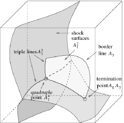
(b)

Figure 2: Typical aspect of the singularities present at a fixed time in the solution for (a) $d=2$ and (b) $d=3$.

The generic form of such singularities and their typical metamorphoses occurring in the course of time were studied in details and classified for $d=2$ and $d=3$ by Arnold, Baryshnikov and Bogaevsky in the Appendix of [62] and in a more detailed paper by Bogaevsky [17]. This classification is based on two criteria: (i) the number of trajectories minimizing (2.5) and (ii) the multiplicity of each of these minima. The shocks corresponding to locations with two distinct minimizers are hence denoted by $A_{1}^{2}$. At a fixed time, the $A_{1}^{2}$ singularities are discrete points in one dimension. In two dimensions (see figure 2(a)) they form curve segments with extremities that can be either triple points $A_{1}^{3}$ or isolated termination points of the type $A_{3}$ corresponding to a degenerate minimum. In three dimensions (see figure 2(b)) the singular manifold is formed by shock surfaces of $A_{1}^{2}$ points. The boundaries of these surfaces are either made of degenerate $A_{3}$ points or of triple lines made of $A_{1}^{3}$ points. The triple lines intersect at isolated $A_{1}^{4}$ points or intersect shock boundaries at particular singularities called $A_{1}A_{3}$ where the minimum is attained in two points, one of which is degenerate.

It is important to remark here that degenerate singularities (of the type $A_{3}$ or of higher orders $A_{5}$, $A_{7}$, etc.) introduce in the solution points where the velocity gradients becomes arbitrarily large. This is not the case of the $A_{1}^{n}$ singularities which correspond to discontinuities of the velocity but are associated to bounded values of its gradients. As we will see in sections 4 and 7, these degenerate singularities are responsible for an algebraic behavior of the probability density function of velocity gradients, velocity increments and of the mass density.

(a)

(b)

Figure 3: Illustration of the similarities between the singular manifold in space time for $d=1$ and at fixed time for $d=2$ (b). The two manifolds contain the same type of singularities with the same co-dimensions. The restrictions on the possible metamorphoses in dimension $d=1$ are the following: a point of the type $A_{3}$ can only exist at the bottom extremity of a shock trajectory; the $A_{1}^{3}$ points necessarily correspond to the merger of two shocks; shock trajectories cannot have a horizontal tangent.

The singularities with co-dimensions $(d+1)$ generically appear in the solution at isolated times. They correspond to instantaneous changes in the topological structure of the singular manifold, called metamorphoses and can be also classified (see [17]). In one dimension, there are two generic metamorphoses: shock formations (the preshocks) corresponding to a specific space-time location where the minimum is degenerate ($A_{3}$ singularities) and shock mergers associated to space-time positions where the minimum is attained for three different trajectories ($A_{1}^{3}$ singularities). We see that some of the singularities generically present in two dimensions appear at isolated times in three dimensions. Actually, all the singularities generically present in dimension $(d+1)$ appear in dimension $d$ on a discrete set of space time, that is at isolated positions and instants of time. However, it has been shown in [17] that the irreversible dynamics of the Burgers equation restricts the set of possible metamorphoses. The admissible metamorphoses are characterized by the following property: after the bifurcation, the singular manifold must remain locally contractible (homotopic to a point in the neighborhood of the Eulerian location of the metamorphosis). This topological restriction is illustrated for the one-dimensional case in figure 3. Note that this constraint actually holds for all solutions to the Hamilton–Jacobi equation in the limit of vanishing viscosity, as long as the Hamiltonian is a convex function.

In order to determine precisely how all these singularities contribute to the statistical properties of the solution, it is important to know the local structure of the velocity (or potential) field in their vicinity. Various normal forms can be obtained from the multiplicity of the minimum in the variational formulation of the solution (2.5). In the case without forcing, they can be obtained from a Taylor expansion of the initial velocity potential. This will be used in next section to determine the tail of the probability distribution of a mass density field advected by a velocity solution to the Burgers equation.

2.4 Remarks on numerical methods

All the traditional methods used to solve equations of fluid dynamics, or more generally any partial differential equations, can be used to obtain the solutions to the Burgers equation. However, as we have seen above, the solution typically has singularities (discontinuities of the velocity) in the limit of vanishing viscosity. Hence methods which rely on the smoothness of the solution require a non-vanishing viscosity, which is introduced either in an explicit way to ensure stability (as, e.g., for pseudo-spectral methods) or in an implicit way through the discretization procedure (as for finite-differences methods). In both cases the value of the viscosity is determined from the mesh size and, even in one dimension, their uses might be very disadvantageous. We will now demonstrate various numerical methods that allow approximating the solutions to the Burgers equation directly in the limit of vanishing viscosity $\nu\to 0$.

2.4.1 Finite volumes

The one-dimensional Burgers equation with no forcing is a scalar conservation law. Its entropic solutions (or viscosity solutions) can thus be approximated numerically by finite-volume methods. Instead of constructing a discrete approximation of the solution on a grid, such methods consist in considering an approximation of its mean value on a discrete partitioning of the system into finite volumes. One then needs to evaluate for each of these volumes the fluxes exchanged with each of its neighbors. Various approximations of these fluxes were introduced by Godunov, Roe, and Lax and Wendroff (see, e.g., [35], Vol. 3, for a review). These methods require to dicretize both space and time. The time step being then related to the spatial mesh size by a Courant–Friedrichs–Lewy type condition. Thus to integrate the equation during times comparable to one eddy turnover time, they require a computational time $O(N^{2})$ where $N$ is the resolution. As we now show there actually exist numerical schemes that allow constructing the solution to the decaying Burgers equation for arbitrary times without any need to compute the solution at intermediate times.

2.4.2 Fast Legendre transform

As we have seen in section 2.1, the solution to the unforced Burgers equation is given explicitly by the variational principle (2.9). A method based on the idea of using this formulation together with a monotonicity property of the Lagrangian map $\vec{x}_{0}\to\vec{x}=\vec{X}(\vec{x}_{0},t)$ was given in [94]. It is called the fast Legendre transform whose principles were already sketched in [23]. Both Eulerian and Lagrangian positions are discretized on regular grids. Then, for a fixed Eulerian location $\vec{x}^{(i)}$ on the grid, one has to find the corresponding Lagrangian coordinate $\vec{x}_{0}^{(j)}$ maximizing (2.9). A naive implementation would require $O(N_{\rm E}^{d}\,N_{\rm L}^{d})$ operations if the Eulerian and the Lagrangian grids contain $N_{\rm E}^{d}$ and $N_{\rm L}^{d}$ points respectively. Actually the number of operations can be reduced to $O((N_{\rm E}\,\ln N_{\rm L})^{d})$ by using the monotonicity of the Lagrangian map, that is the fact that for any pair of Lagrangian positions $\vec{x}_{0}^{(1)}$ and $\vec{x}_{0}^{(2)}$, one has at any time $[\vec{X}(\vec{x}_{0}^{(1)},t)-\vec{X}(\vec{x}_{0}^{(2)},t)]\cdot(\vec{x}_{0}^{(1)}-\vec{x}_{0}^{(2)})\geq 0$. In the case of orthogonal grids, this property allows performing the maximization by exploring along a binary tree the various possibilities; thus the number of operations is reduced to $\ln N_{\rm L}$ for each of the $N_{\rm E}$ positions on the Eulerian grid. Such algorithms give access to the solution not only directly in the limit of vanishing viscosity but also by jumping directly from the initial time to an arbitrary time.

This method can also be used for the forced Burgers equation, approximating the forcing by a sum of impulses at discrete times and letting the solution decay between two such kicks. This gives an efficient algorithm for the forced Burgers equation directly applicable in the limit of vanishing viscosity.

2.4.3 Particle tracking methods

In one dimension, Lagrangian methods can be implemented in a straightforward manner after noticing that particles cannot cross each other and that it is advisable to track not only fluid particles but also shocks (see, e.g., [6]). Lagrangian methods can in principle be used to solve the Burgers equation in any dimension. However the shock dynamics is meaningful only for potential solutions. Outside the potential framework almost nothing is known about the construction of the solution beyond the first crossing of trajectories. In the potential case, a particle method can be formulated by choosing to represent the solution in the position-potential $(\vec{x},\Psi)$ space instead of the position-velocity $(\vec{x},\vec{v})$ space. An idea in two dimensions, which was not yet implemented, consists in considering a meshing of the hyper-surface defined by the velocity potential. If such a mesh contains only triple points, such singularities are preserved by the dynamics and can be tracked using the results discussed below in section 4.2 and by checking at all time steps in an exhaustive manner at all the metamorphoses encountered by triple points.

3 Decaying Burgers turbulence

We focus in this section on the solutions to the $d$-dimensional unforced potential Burgers equation

$$\partial_{t}\vec{v}+\vec{v}\!\cdot\!\nabla\vec{v}=\nu\nabla^{2}\vec{v},\ \ \vec{v}(\vec{x},0)\!=\!\vec{v}_{0}(\vec{x})\!=\!-\nabla\Psi_{0}(\vec{x}).$$ (3.1)

As showed in section 2.1, the solution can be expressed in the limit of vanishing viscosity $\nu\to 0$ in terms of a variational principle that relates the velocity potential at time $t$ to its initial value:

$$\Psi({\vec{x}},t)=\max_{{\vec{x}}_{0}}\left(\Psi_{0}({\vec{x}}_{0})-\frac{|{\vec{x}}-{\vec{x}}_{0}|^{2}}{2t}\right).$$ (3.2)

The next subsection describes several geometrical constructions of the solution that are helpful to determine various statistical properties of the decaying problem (3.1). This is illustrated in subsections 3.2 and 3.3 which are devoted to the study of the decay of smooth homogeneous and of Brownian initial data, respectively.

The study of the solutions to the Burgers equation transporting a density field is of particular interest in the application of the Burgers equation in cosmology within the framework of the adhesion model. This question will be discussed in section 4.

3.1 Geometrical constructions of the solution

3.1.1 The potential Lagrangian manifold

The variational formulation of the solution (3.2) has a simple geometrical interpretation in the position-potential space $({\vec{x}},\Psi)$ of dimension $d+1$. Indeed, consider the $d$-dimensional manifold parameterized by the Lagrangian coordinate ${\vec{x}}_{0}$ and defined by

$$\left\{\begin{array}[]{lll}{\vec{x}}&=&{\vec{x}}_{0}-t\,\nabla\Psi_{0}({\vec{x}}_{0})\\ \Psi&=&\displaystyle\Psi_{0}({\vec{x}}_{0})-\frac{t}{2}|\nabla\Psi_{0}({\vec{x}}_{0})|^{2}.\end{array}\right.$$ (3.3)

The first line corresponds to the position where the gradient of the argument of the maximum function in (3.2) vanishes while the second line is just its argument evaluated at the maximum. For a sufficiently regular initial potential $\Psi_{0}$ (at least twice differentiable) and for sufficiently small times, equation (3.3) unambiguously defines a single-valued function $\Psi({\vec{x}},t)$. However, there exists generically a time $t_{\star}$ at which the manifold is folding. Figure 4(a) (upper) shows in one space dimension the typical shape of the Lagrangian manifold defined by (3.3) after the critical time $t_{\star}$. For some Eulerian positions ${\vec{x}}$, there is more than one branch and cusps are present at Eulerian locations where the number of branches change.

(a)

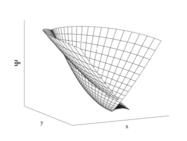
(b)

Figure 4: (a) Lagrangian manifold for $d=1$ in the $(x,\Psi)$ plane (upper) and in the $(x,v)$ plane (lower); the heavy lines correspond to the correct Eulerian solutions. (b) Lagrangian manifold in the $({\vec{x}},\Psi)$ space for $d=2$.

The situation is very similar in higher dimensions as illustrated for $d=2$ in figure 4(b). Clearly from the variational principle (2.9), the correct solution to the inviscid Burgers equation is obtained by taking the maximum, that is the highest branch. The velocity potential is by construction always continuous but it contains angular points corresponding to discontinuities of the velocity ${\vec{v}}=-\nabla\Psi$. Such singularities are located at Eulerian locations where the maximum in (2.9) is degenerate and attained for different ${\vec{x}}_{0}$. As already discussed in section 2.3 the different singularities appearing in the solutions can be classified in any dimension.

Below we describe other geometrical constructions of the solutions to the decaying Burgers equation in the limit of vanishing viscosity that are based on the variational principle (2.9).

3.1.2 The velocity Lagrangian manifold

In one dimension, when the velocity field is always potential, the method based on the study of the potential manifold in the $(x,\Psi)$ space described above can be straightforwardly extended to the position-velocity phase space. Consider the Lagrangian manifold defined by

$$\left\{\begin{array}[]{lll}x&=&x_{0}-t\,v_{0}(x_{0})\\ v&=&v_{0}(x_{0}).\end{array}\right.$$ (3.4)

The regular parts of the graph of the solution are necessarily contained in this manifold. However, for times larger than $t_{\star}$, folding appears and the naive solution would be multi-valued. To construct the true solution one should find a way to choose among the different branches. In one dimension, there is a simple relation between the potential Lagrangian manifold in the $(x,\Psi)$ plane and those of the $(x,v)$ plane defined by (3.4): the potential manifold is obtained by taking the “multi-valued integral” that can be defined by transforming the spatial integral into an integral with respect to the arc length. The maximum representation (2.9) implies that the velocity potential is continuous. Hence a shock corresponds to an Eulerian position $x$ where two points belonging to different branches define equal areas in the $(x,v)$ plane. In the case of a single loop of the manifold, this is equivalent to applying the Maxwell rule to determine the shock position (see figure 4(a) - lower). This construction of the solution can become rather involved as soon as the number of shocks becomes large or that several mergers have taken place. For the moment there is no generalization to dimension higher than one of this Maxwell rule construction of the solution. For such an extension, one needs to develop a geometrical framework to describe the Lagrangian manifold in the $({\vec{x}},{\vec{v}})$ space. Such approaches would certainly shed some light on the problem of constructing non-potential solutions to the Burgers equation in the limit of vanishing viscosity.

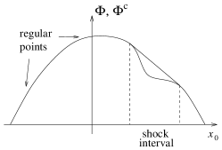
(a)

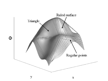
(b)

Figure 5: Convex hull construction in terms of the Lagrangian potential (a) for $d=1$ and (b) for $d=2$.

3.1.3 The convex hull of the Lagrangian potential

Another geometrical construction of the solution, which is valid in any dimension makes use of the Lagrangian potential

$$\Phi({\vec{x}}_{0},t)=t\Psi_{0}({\vec{x}}_{0})-\frac{|{\vec{x}}_{0}|^{2}}{2}.$$ (3.5)

Clearly, the negative gradient of the Lagrangian potential gives the naive Lagrangian map

$$\vec{X}({\vec{x}}_{0},t)=-\nabla_{{\vec{x}}_{0}}\Phi({\vec{x}}_{0},t)={\vec{x}}_{0}+t{\vec{v}}_{0}({\vec{x}}_{0}),$$ (3.6)

that is satisfied by Lagrangian trajectories as long as they do not enter shocks. The maximum formulation of the solution (2.9) can be rewritten as

$$t\Psi({\vec{x}},t)+\frac{|{\vec{x}}|^{2}}{2}=\max_{{\vec{x}}_{0}}(\Phi({\vec{x}}_{0})+{\vec{x}}_{0}\cdot{\vec{x}}),$$ (3.7)

which represents the potential as, basically, a Legendre transform of the Lagrangian potential. An important property of the Legendre transform is that the right-hand side. of (3.7) is unchanged if the Lagrangian potential $\Phi$ is replaced by its convex hull, that is the intersection of all the half planes containing its graph. In other terms, the convex hull $\Phi^{\rm c}$ of the Lagrangian potential $\Phi$ is defined as $\Phi^{\rm c}({\vec{x}}_{0},t)=\inf g({\vec{x}}_{0})$, where the infimum is taken over all convex functions $g$ satisfying $g(\cdot)\geq\Phi(\cdot,t)$. This is illustrated in one dimension in figure 5(a) which shows both regular points (Lagrangian points which have not fallen into a shock) and one shock interval, situated below the segment which is a part of the convex hull. In two dimensions, as illustrated in figure 5(b), the convex hull is typically formed by regular points, by ruled surfaces, and by triangles which correspond, to the regular part of the velocity field, the shock lines, and the shock nodes, respectively.

Note that in one dimension, there exists an equivalent construction which is directly based on the Lagrangian map $x_{0}\mapsto X(x_{0},t)$ defined by (3.6). Working with the convex hull is equivalent to the Maxwell rule applied to the non-invertible regions of the Lagrangian map. A shock corresponds to a whole Lagrangian interval having a single point as an Eulerian image. One then talks about a Lagrangian shock interval.

3.1.4 The paraboloid construction

Finally, the maximum representation (3.7) leads in a straightforward way to another geometrical construction of the solution. As illustrated in figure 6 in both one and two dimensions, a paraboloid with apex at ${\vec{x}}$ and radius of curvature proportional to $t$ is moved down in the $({\vec{x}}_{0},\Psi_{0})$ space until it touches the surface defined by the initial velocity potential $\Psi_{0}$ at the Lagrangian location associated to ${\vec{x}}$. The location ${\vec{x}}_{0}$ where the paraboloid touches the graph of the potential is exactly the pre-image of ${\vec{x}}$. If it touches simultaneously at several locations, a shock is located at the Eulerian position ${\vec{x}}$. One constructs in this way the inverse Lagrangian map.

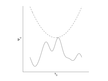
(a)

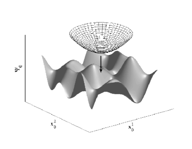
(b)

Figure 6: Paraboloid construction of solution for (a) $d=1$ and (b) $d=2$.

3.2 Kida’s law for energy decay

An important issue in turbulence is that of the law of decay at long times when the viscosity is very small. Before turning to the Burgers equation it is useful to recall some of the features of decay for the incompressible Navier–Stokes case. It is generally believed that high-Reynolds number turbulence has universal and non-trivial small-scale properties. In contrast, large scales, important for practical applications such as transport of heat or pollutants, are believed to be non-universal. This is however so only for the toy model of turbulence maintained by prescribed large-scale random forces. Very high-Reynolds number turbulence, decaying away from its production source, and far from boundaries can relax under its internal nonlinear dynamics to a (self-similarly evolving) state with universal and non-trivial statistical properties at all scales. Von Kármán and Howarth [109], investigating the decay for the case of high-Reynolds number homogeneous isotropic three-dimensional turbulence, proposed a self-preservation (self-similarity) ansatz for the spatial correlation function of the velocity: the functional shape of the correlation function remains fixed, while the integral scale $L(t)$ grows in time and the mean kinetic energy $E(t)=V^{2}(t)$ decays, both following power laws; there are two exponents which can be related by the condition that the energy dissipation per unit mass $|\dot{E}(t)|$ should be proportional to $V^{3}/L$. But an additional relation is needed to actually determine the exponents. The invariance in time of the energy spectrum at low wavenumbers, known as the “permanence of large eddies” [53, 84, 63] can be used to derive the law of self-similar decay when the initial spectrum $E_{0}(k)\propto k^{n}$ at small wavenumbers $k$ with $n$ below a critical value equal to 3 or 4, the actual value being disputed because of the “Gurbatov phenomenon” (see the end of this section). One then obtains a law of decay $E(t)\propto t^{-2(n+1)/(3+n)}$. (Kolmogorov [79] proposed a law of energy decay $V^{2}(t)\propto t^{-10/7}$, which corresponds to $n=4$ and used in its derivation the so-called “Loitsyansky invariant”, a quantity actually not conserved, as shown by Proudman and Reid [100].) When the initial energy spectrum at low wavenumbers goes to zero too quickly, the permanence of large eddies cannot be used, because the energy gets backscattered to low wavenumbers by nonlinear interactions. For Navier–Stokes turbulence the true law of decay is then known only within the framework of closure theories (see, e.g., [84]).

For one-dimensional Burgers turbulence, many of the above issues are completely settled. First, we observe that the problem of decay is quite simple if spatial periodicity is assumed. Indeed, all the shocks appearing in the solution will eventually merge into a single shock per period, as shown in figure 7. The position of this shock is random and the two ramps have slope $1/t$, as is easily shown using the parabola construction of subsection 3.1. Hence, the law of decay is simply $E(t)\propto t^{-2}$.

Figure 7: Snapshot of solution of decaying Burgers turbulence at long times when spatial periodicity is assumed.

Nontrivial laws of decay are obtained if the Burgers turbulence is homogeneous in an unbounded domain and has the “mixing” property (which means, roughly, that correlations are vanishing when the separation goes to infinity). The number of shocks is then typically infinite but their density per unit length decreases in time because shocks are constantly merging. The $E(t)\propto t^{-2(n+1)/(3+n)}$ law mentioned above can be derived for Burgers turbulence from the permanence of large eddies when $n\leq 1$ [63]. For $n=0$, this $t^{-2/3}$ law was actually derived by Burgers himself [27].

The hardest problem is again when permanence of large eddies does not determine the outcome, namely for $n>1$. This problem was solved by Kida [77] (see also [51, 61, 63]).

We now give some key ideas regarding the derivation of Kida’s law of energy decay. We assume Gaussian, homogeneous smooth initial conditions, such that the potential is homogeneous. Note that a homogeneous function is not, in general, the derivative of another homogeneous function. Here this is guaranteed by assuming that the initial spectrum of the kinetic energy is of the form

$$E_{0}(k)\propto k^{n}\mbox{ for }k\to 0\mbox{ with }n>1\,.$$ (3.8)

This condition implies that the mean square initial potential $\int k^{-2}E_{0}(k)\,\mathrm{d}k$ has no infrared (small-$k$) divergence (the absence of an ultraviolet divergence is guaranteed by the assumed smoothness).

A very useful property of decaying Burgers turbulence, which has no counterpart for Navier–Stokes turbulence, is the relation

$$E(t)=\frac{\partial}{\partial t}\left\langle\Psi\right\rangle,$$ (3.9)

which follows by taking the mean of the Hamilton–Jacobi equation for the potential (2.2) in the absence of viscosity and of a driving force. Hence, the law of energy decay can be obtained from the law for the mean potential. The latter can be derived from the cumulative probability of the potential which, by homogeneity, does not depend on the position. By (2.9), its expression at $x=0$ is

$$\mbox{Prob}\!\left\{\mbox{Pot.}\!<\!\Psi\right\}\!=\!\mbox{Prob}\!\left\{\!\forall x_{0},\,\Psi_{0}(x_{0})\!<\!\frac{x_{0}^{2}}{2t}\!+\!\Psi\right\}\!.$$ (3.10)

Expressed in words, we want to find the probability that the initial potential does not cross the parabola $x_{0}^{2}/(2t)+\Psi$ (see figure 8).

Figure 8: An initial potential which is everywhere below the parabola $x_{0}^{2}/(2t)+\Psi$. The probability of such events gives the cumulative probability to have a potential at time $t$ less than $\Psi$.

Since, at large times $t$, the relevant $\Psi$ is going to be large, the problem becomes that of not crossing a parabola with small curvature and very high apex. The crossings, more precisely the up-crossings, are spatially quite rare and, for large $t$, form a Poisson process [92] for which

$$\hbox{Prob. no crossing}\simeq\mathrm{e}^{-\left\langle N(t)\right\rangle},$$ (3.11)

where $\left\langle N(t)\right\rangle$ is the mean number of up-crossings. By the Rice formula (a consequence of the identity $\delta(\lambda x)=(1/|\lambda|)\delta(x)$),

$$\left\langle N(t)\right\rangle\!=\!\left\langle\int_{-\infty}^{+\infty}\!\!\!\mathrm{d}x_{0}\,\delta\!\left(m(x_{0})\!-\!\Psi\right)\frac{\mathrm{d}m}{\mathrm{d}x_{0}}\mathrm{H}\!\left(\!\frac{\mathrm{d}m}{\mathrm{d}x_{0}}\!\right)\!\right\rangle\!,$$ (3.12)

where $\mathrm{H}$ is the Heaviside function and

$$m(x_{0})\equiv\Psi_{0}(x_{0})-\frac{x_{0}^{2}}{2t}.$$ (3.13)

Since $\Psi_{0}(x_{0})$ is Gaussian, the right-hand side of (3.12) can be easily expressed in terms of integrals over the probability densities of $\Psi_{0}(x_{0})$ and of $\mathrm{d}\Psi_{0}(x_{0})/\mathrm{d}x_{0}$ (as a consequence of homogeneity these variables are uncorrelated and, hence, independent). The resulting integral can then be expanded by Laplace’s method for large $t$, yielding

$$\left\langle N(t)\right\rangle\sim t^{1/2}\Psi^{-1/2}e^{-\Psi^{2}},\quad t\to\infty.$$ (3.14)

When this expression is used in (3.11) and the result is differentiated with respect to $\Psi$ to obtain the probability density function (PDF) of $p(\Psi)$, the latter is found to be concentrated around $\Psi_{\star}=(\ln t)^{1/2}$. It then follows that, at large times, we obtain Kida’s log-corrected $1/t$ law for the energy decay

$$\left\langle\Psi\right\rangle\sim(\ln t)^{1/2}\!,\ E(t)\sim\frac{1}{t(\ln t)^{1/2}}\!,\ L(t)\sim\left[\frac{t}{\ln t}\right]^{1/4}\!\!\!\!\!\!\!\!\!.$$ (3.15)

Figure 9: The Eulerian solution at large times $t$. The ramps have slope $1/t$. In time-independent scales, the figure would be stretched horizontally and squeezed vertically by a factor proportional to $t$.

The Eulerian solution, at large times, has the ramp structure shown in figure 9 with shocks of typical strength $V(t)=E^{1/2}(t)$, separated by a distance $L(t)$.

The fact that Kida’s law is valid for any $n>1$, and not just for $n\geq 2$ as thought originally, gives rise to an interesting phenomenon now known as the “Gurbatov effect”: if $1<n<2$ the large-time evolution of the energy spectrum cannot be globally self-similar. Indeed, the permanence of large eddies, which is valid for any $n<2$ dictates that the spectrum should preserve exactly its initial $C_{n}k^{n}$ behavior at small wavenumbers $k$, with a constant-in-time $C_{n}$. Global self-similarity would then imply a $t^{-2(n+1)/(3+n)}$ law for the energy decay, which would contradict Kida’s law. Actually, as shown in [63], there are two characteristic wavenumbers with different time dependences, the integral wavenumber $k_{L}(t)\sim(L(t))^{-1}$ and a switching wavenumber $k_{s}(t)$ below which holds the permanence of large eddies. It was shown that the same phenomenon is present also in the decay of a passive scalar [45]. Whether or not a similar phenomenon is present in three-dimensional Navier–Stokes incompressible turbulence, or even in closure models, is a controversial matter [44, 97].

For decaying Burgers turbulence, if we leave aside the Gurbatov phenomenon which does not affect energy-carrying scales, the following may be shown. If we rescale distances by a factor $L(t)$ and velocity amplitudes by a factor $V(t)=E^{1/2}(t)$ and then let $t\to\infty$, the spatial (single-time) statistical properties of the whole random velocity field become time-independent. In other words, there is a self-similar evolution at large times. Hence, dimensionless ratios such as the velocity flatness

$$F(t)\equiv\frac{\left\langle v^{4}(t)\right\rangle}{\left[\left\langle v^{2}(t)\right\rangle\right]^{2}}$$ (3.16)

have a finite limit as $t\to\infty$. A similar property holds for the decay of passive scalars [28]. We do not know if this property holds also for Navier–Stokes incompressible turbulence or if, say, the velocity flatness grows without bounds at large times.

3.3 Brownian initial velocities

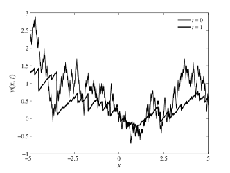
(a)

(b)

Figure 10: Snapshot of the solution resulting from Brownian initial data in one dimension. (a) Velocity profile at initial time $t=0$ and at time $t=1$; notice the dense proliferation of shocks. (b) Lagrangian potential together with its convex hull.

Initial conditions in the Burgers equation that are Gaussian with a power-law spectrum $\propto k^{-\alpha}$ have been frequently studied because they belong in cosmology to the class of scale-free initial conditions (see [98, 34]). We consider here the one-dimensional case with Brownian motion as initial velocity, corresponding to $\alpha=2$.

Brownian motion is continuous but not differentiable; thus, shocks appear after arbitrarily short times and are actually dense (see figure 10(a)). Numerically supported conjectures made in [104] have led to a proof by Sinai [105] of the following result: in Lagrangian coordinates, the regular points, that is fluid particles which have not yet fallen into shocks, form a fractal set of Hausdorff dimension $1/2$. This implies that the Lagrangian map forms a Devil’s staircase of dimension $1/2$ (see figure 11). Note that when the initial velocity is Brownian, the Lagrangian potential has a second space derivative delta-correlated in space; this can be approximately pictured as a situation where the Lagrangian potential has very wild oscillations in curvature. Hence, it is not surprising that very few points of its graph can belong to its convex hull (see figure 10(b)).

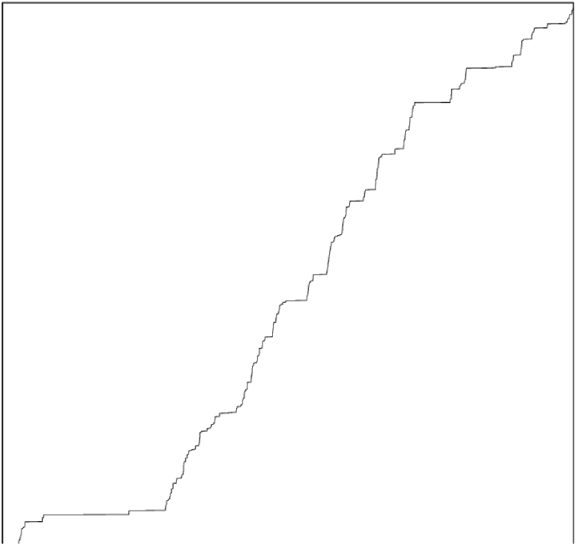
Figure 11: The Lagrangian map looks like a Devil’s staircase: it is constant almost everywhere, except on a fractal Cantor-like set (from [107]).

We will now highlight some aspects of Sinai’s proof of this result. The idea is to use the construction of the solution in terms of the convex hull of the Lagrangian potential (see section 3.1), so that regular points are exactly points where the graph of the Lagrangian potential coincides with its convex hull. For this problem, the Hausdorff dimension of the regular points is also equal to its box-counting dimension, which is easier to determine. One obtains it by finding the probability that a small Lagrangian interval of length $\ell$ contains at least one regular point which belongs simultaneously to the graph of the Lagrangian potential $\Phi$ and to its convex hull. In other words, one looks for points, such as $R$, with the property that the graph of $\Phi$ lies below its tangent at $R$ (see figure 12). Following Sinai, this can be equivalently formulated by the box construction with the following constraints on the graph:
Left:  graph of the potential below the half line $\Gamma_{-}$,
Right:  graph of the potential below the half line $\Gamma_{+}$,
Box:  $\!\!\left\{\!\begin{array}[]{ll}1:&\mbox{enter }(AF)\mbox{ with a slope larger}\\[-5.0pt] &\mbox{than that of }\Gamma_{-}\mbox{ by }O(\ell^{1/2})\\[-2.0pt] 2:&\mbox{exit }(CB)\mbox{ with a slope less than}\\[-5.0pt] &\mbox{that of }\Gamma_{+}\mbox{ by }O(\ell^{1/2})\\[-2.0pt] 3:&\mbox{cross }(FC)\mbox{ and stay below }(ED).\end{array}\right.$
It is obvious that such conditions ensure the existence of at least one regular point, as seen by moving $(ED)$ down parallel to itself until it touches the graph. Note that $A$ and the slope of $(AB)$ are prescribed. Hence, one is calculating conditional probabilities; but it may be shown that the conditioning is not affecting the scaling dependence on $\ell$.

Figure 12: The box construction used to find a regular point $R$ within a Lagrangian interval of length $\ell$ (from [105, 107]).

As the Brownian motion $v_{0}(x_{0})$ is a Markov process, the constraints Left, Box and Right are independent and hence,

$$P^{\rm reg.} \!(\ell)\equiv{\rm Prob}\!\left\{\mbox{regular point in interval of length }\ell\right\}$$ (3.17)

$$={\rm Prob}\!\left\{\mbox{\sl Left}\right\}\!\times\!{\rm Prob}\!\left\{\mbox{\sl Box}\right\}\!\times\!{\rm Prob}\!\left\{\mbox{\sl Right}\right\}.$$

The sizes of the box were chosen so that ${\rm Prob}\left\{\mbox{\sl Box}\right\}$ is independent of $\ell$:

$${\rm Prob}\left\{\mbox{\sl Box}\right\}\sim\ell^{0}.$$ (3.18)

Indeed, Brownian motion and its integral have scaling exponent $1/2$ and $3/2$, respectively, and the problem with $\ell\ll 1$ can be rescaled into that with $\ell=1$ without changing probabilities.

It is clear by symmetry that ${\rm Prob}\!\left\{\mbox{\sl Left}\right\}$ and ${\rm Prob}\!\left\{\mbox{\sl Right}\right\}$ have the same scaling in $\ell$. Let us concentrate on ${\rm Prob}\!\left\{\mbox{\sl Right}\right\}$. We can write the equation for the half line $\Gamma_{+}$ in the form

$$\Gamma_{+}\!\!:x_{0}\mapsto \Phi(x_{0}^{\prime\prime})\!+\!\delta\ell^{3/2}$$ (3.19)

$$\!+\!\left[\frac{\mathrm{d}\Phi}{\mathrm{d}x_{0}}(x_{0}^{\prime\prime})\!+\!\gamma\ell^{1/2}\right]\!(x_{0}\!-\!x_{0}^{\prime\prime}),$$

where $\gamma$ and $\delta$ are positive $O(1)$ quantities. Hence, introducing $\alpha\equiv x_{0}-x_{0}^{\prime\prime}$, the condition Right can be written to the leading order as

$$\int_{0}^{\alpha}\!\!\!\left[v_{0}(x_{0})+\gamma\ell^{1/2}\right]\!\mathrm{d}x_{0}+\delta\ell^{3/2}+\frac{\alpha^{2}}{2}>0,$$ (3.20)

for all $\alpha>0$. By the change of variable $\alpha=\beta\ell$ and use of the fact that the Brownian motion has scaling exponent $1/2$, one can write the condition Right as

$$\int_{0}^{\beta}\left(v_{0}(x_{0})+\gamma\right)\mathrm{d}x_{0}>-\delta,\mbox{ for all }\alpha\in[0,\ell^{-1}].$$ (3.21)

Without affecting the leading order, one can replace the Brownian motion by a stepwise constant random walk with jumps of $\pm 1$ at integer $x_{0}$’s. The integral in (3.21) has a simple geometric interpretation, as highlighted in figure 13, which shows a random walk starting from the ordinate $\gamma$ and the arches determined by successive zero-passings. The areas of these arches are denoted $S_{\star},S_{1},...S_{n},S_{\star\star}$.

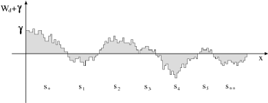
Figure 13: The arches construction which uses the zero-passings of a random walk to estimate the integral of Brownian motion (from [105, 107]).

It is easily seen that

$${\rm Prob}\!\left\{\mbox{\sl Right}\right\}\sim{\rm Prob}\{S_{1}>0,\,S_{1}+S_{2}>0,\,\ldots$$

$$S_{1}+\cdots+S_{n}>0 \!\},$$ (3.22)

where $n=O(\ell^{-1/2})$ is the number of zero-passings of the random walk in the interval $[0,\ell^{-1}]$. The probability (3.22) can be evaluated by random walk methods (see, e.g.,[49], Chap. 12, section 7), yielding

$${\rm Prob}\!\left\{\mbox{\sl Right}\right\} \sim {\rm Prob}\!\left\{n\mbox{ first sums}\!>\!0\right\}$$ (3.23)

$$\propto n^{-1/2}\propto\ell^{1/4}\!\!.$$

By (3.17), (3.18) and (3.23), the probability to have a regular point in a small interval of length $\ell$ behaves as $\ell^{1/2}$ when $\ell\to 0$. Thus, the regular points have a box-counting dimension $1/2$.

This rigorous result on the fractal dimension of regular points served as a basis in [4] for a proof of the bifractality of the inverse Lagrangian map when the initial velocity is Brownian. Namely, the moments $M_{q}(\ell)=\left\langle(x_{0}(x+\ell)-x_{0}(x))\right\rangle$ behave as $\ell^{\tau_{q}}$ at small separation $\ell$ and the exponents $\tau_{q}$ experience the phase transition

$$\tau_{q}=2q\mbox{ for }q\leq 1/2$$ (3.24)

$$\tau_{q}=1\mbox{ for }q\geq 1/2$$ (3.25)

At the moment, this is the only rigorous result on the bifractal nature of the solutions to the Burgers equation in the case of non-differentiable initial velocity. In particular, the case of fractional Brownian motion is still opened.

4 Transport of mass in the Burgers/adhesion model

In the cosmological application of the Burgers equation, i.e. for the adhesion model, it is of particular interest to analyze the behavior of the density of matter, since the large-scale structures are characterized as regions where mass is concentrated. This is done by associating to the velocity field ${\vec{v}}$ solution to the $d$-dimensional decaying Burgers equation (3.1), a continuity equation for the transport of a mass density field $\rho$. In Eulerian coordinates, the mass density $\rho$ satisfies

$$\partial_{t}\rho+\nabla\cdot(\rho\vec{v})=0\,,\quad\rho(\vec{x},0)=\rho_{0}(\vec{x})\,.$$ (4.1)

A straightforward consequence of (4.1) and of the formulation of Burgers dynamics in terms of characteristics $\vec{X}(\vec{x}_{0},t)$ is that, at the Eulerian locations where the Lagrangian map is invertible, the mass density field $\rho$ can be expressed as

$$\rho(\vec{x},t)\!=\!\frac{\rho_{0}(\vec{x}_{0})}{J(\vec{x}_{0},t)}, \mbox{where }\vec{X}(\vec{x}_{0},t)\!=\!\vec{x},$$

and $$J(\vec{x}_{0},t)\!=\!\det\!\left[(\partial X^{i})/(\partial x_{0}^{j})\right]\!\!.$$ (4.2)

Large but finite values of the density will be reached at locations where the Jacobian $J$ of the Lagrangian map becomes very small. As we will see in section 4.1, they contribute a power-law behavior in the tail of the probability density function of $\rho$.

The expression (4.2) is no more valid when the Jacobian vanishes (inside shocks). Then the density field becomes infinite and mass accumulates on the shock. We will see in section 4.2 that the evolution of the mass inside the singularities of the solution can be obtained as the $\nu\to 0$ limit of the well-posed viscous problem. Finally, we will discuss in section 4.3 some of the applications of the Burgers equation to cosmology, and in particular how, assuming the dynamics of the adhesion model, the question of reconstruction of the early Universe from its present state can be interpreted as a convex optimal mass transportation problem.

4.1 Mass density and singularities

We give here the proof reported in [54] that in any dimension large densities are localized near “kurtoparabolic” singularities residing on space-time manifolds of co-dimension two. In any dimension, such singularities contribute universal power-law tails with exponent $-7/2$ to the mass density probability density function (PDF) $p(\rho)$, provided that the initial conditions are smooth.

In one dimension, the mass density at regular points can be written as

$$\rho(X(x_{0},t),t)=\frac{\rho_{0}(x_{0})}{1-t[(\mathrm{d}^{2}\Psi_{0})/(\mathrm{d}x_{0}^{2})]}\,.$$ (4.3)

We suppose here that the initial density $\rho_{0}$ is strictly positive and that both $\rho_{0}$ and $\Psi_{0}$ are sufficiently regular statistically homogeneous random fields. Large values of $\rho(x,t)$ are obtained in the neighborhood of Lagrangian positions with a vanishing Jacobian, i.e. where $\mathrm{d}^{2}\Psi_{0}(x_{0})/\mathrm{d}x_{0}^{2}=1/t$. Once mature shocks have formed, the Lagrangian points with vanishing Jacobian are inside shock intervals and thus not regular. The only points with a vanishing Jacobian that are at the boundary of the regular points are obtained at the preshocks, that is when a new shock is just born at some time $t_{\star}$. Such points, that we denote by $x_{0}^{\star}$, are local minima of the initial velocity gradient which have to be negative, so that the following relations are satisfied:

$$\frac{\mathrm{d}^{2}\Psi_{0}}{\mathrm{d}x_{0}^{2}}(x_{0}^{\star})=\frac{1}{t_{\star}},\ \frac{\mathrm{d}^{3}\Psi_{0}}{\mathrm{d}x_{0}^{3}}(x_{0}^{\star})=0,\ \frac{\mathrm{d}^{3}\Psi_{0}}{\mathrm{d}x_{0}^{3}}(x_{0}^{\star})<0\,.$$ (4.4)

There is of course an extra global regularity condition that the preshock Lagrangian location $x_{0}^{\star}$ has not been captured by a mature shock at a time previous to $t_{\star}$. This global condition affects only constants but not the scaling behavior of $p(\rho)$ at large $\rho$.

We now Taylor-expand the initial density and the initial velocity potential in the vicinity of $x_{0}^{\star}$. By adding a suitable constant to the initial potential, shifting $x_{0}^{\star}$ to the origin and making a Galilean transformation canceling the initial velocity at $x_{0}^{\star}$, we obtain the following “normal forms” for the Lagrangian potential (3.5) and for the density

$$\Phi(x_{0},t)\!\simeq\!\frac{1}{2}\tau x_{0}^{2}\!+\!\zeta x_{0}^{4},\ \ \rho(X\!(x_{0},t),t)\!\simeq\!\displaystyle\frac{-\rho_{0}}{\tau\!+\!12\zeta x_{0}^{2}},$$ (4.5)

where

$$\tau=\frac{t-t_{\star}}{t_{\star}}\mbox{ and }\zeta=\frac{t_{\star}}{24}\,\left.\frac{\mathrm{d}^{4}\Psi_{0}}{\mathrm{d}x_{0}^{4}}\right|_{x_{0}=0}<0\,.$$ (4.6)

The Lagrangian potential bifurcates from a situation where it has a single maximum at $\tau<0$ through a degenerate maximum with quartic behavior at $\tau=0$, to a situation where convexity is lost and where it has two maxima at $x_{0}^{\pm}=\pm\sqrt{-\tau/(4\zeta)}$ for $\tau>0$. As a result of our choice of coordinates, the symmetry implies that the convex hull contains a horizontal segment joining these two maxima (see. figure 14(a)).

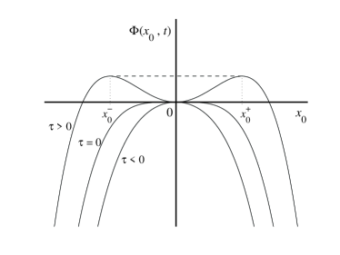
(a)

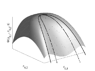
(b)

Figure 14: Normal form of the Lagrangian potential. (a) in one dimension, in the time-neighborhood of a preshock; at the time of the preshock ($\tau=0$), the Lagrangian potential changes from a single extremum to three extrema and develops a non-trivial convex hull (shown as a dashed line). (b) in two dimension, the space neighborhood of a shock ending point has a structure similar to the spatio-temporal normal form of a preshock in one dimension when replacing the $x_{0,2}$ variable by the time $\tau$; the continuous line is the separatrix between the regular part and the ruled surface of the convex hull; the dotted line corresponds to the locations where the Jacobian of the Lagrangian map vanishes.

We see from (4.5) that the Eulerian density $\rho$ is proportional to $x_{0}^{2}$ in Lagrangian coordinates at $t=t_{\star}$. Since $X=-\partial_{x_{0}}\Phi$, the relation between Lagrangian and Eulerian coordinates is cubic, so that at $\tau=0$, the density has a singularity $\propto x^{-2/3}$ in Eulerian coordinates. At any time $t\neq t_{\star}$, the density remains bounded except at the shock position. Before the preshock ($\tau<0$), it is clear that $\rho<-\rho_{0}/\tau$, while after ($\tau>0$), exclusion of the Lagrangian shock interval $[x_{0}^{-},x_{0}^{+}]$ implies that $\rho<\rho_{0}/(2\tau)$. Clearly, large densities are obtained only in the immediate space-time neighborhood of the preshock. More precisely, it follows from (4.5) that having $\rho(x,t)>\mu$ requires simultaneously

$$|\tau|<\frac{\rho_{0}}{\mu}\mbox{ and }|x|<(-12\zeta)^{-1/2}\left(\frac{\rho_{0}}{\mu}\right)^{3/2}\!\!\!.$$ (4.7)

The tail of the cumulative probability of the density can be determined from the fraction of Eulerian space-time where $\rho$ exceeds a given value. This leads to

$$P^{>}\!(\mu;\,x,t)=\mbox{Prob}\!\left\{\rho(x,t)\!>\!\mu\right\}\simeq C(x,t)\mu^{-5/2}\!,$$ (4.8)

where the constant $C$ can be expressed as

$$C(x,t)=A\,t\,\int_{-\infty}^{0}|\zeta|^{-1/2}p_{3}(x,t,\zeta)\,\mathrm{d}\zeta,$$ (4.9)

$A$ is a positive numerical constant and $p_{3}$ designates the joint probability distribution of the preshock space-time position and of its “strength” coefficient $\zeta$ (see [54] for details). This algebraic law for the cumulative probability implies that the PDF of the mass density has a power-law tail with exponent $-7/2$ at large values. Actually this law was first proposed in [37] for the large-negative tail of velocity gradients in one-dimensional forced Burgers turbulence, a subject to which we shall come back in section 7.

In higher dimensions it was shown in [54] that the main contribution to the probability distribution tail of the mass density does not stem from preshocks but from “kurtoparabolic” points. Such singularities (called $A_{3}$ according to the classification of [62], which is summarized in section 2.3) correspond to locations which belong to the regular part of the convex hull of the Lagrangian potential $\Phi(\vec{x}_{0},t)$ and where its Hessian vanishes. The name kurtoparabolic comes from the Greek “kurtos” meaning “convex”. These points are located on the spatial boundaries of shocks and generically form space-time manifolds of co-dimension 2 (persisting isolated points for $d=2$, lines for $d=3$, etc.). As in one dimension, the normal form of such singularities is obtained by Taylor-expanding in a suitable coordinate frame the Lagrangian potential to the relevant order

$$\Phi(\vec{x}_{0},t)\simeq\zeta x_{0,1}^{4}\!+\!\!\sum_{2\leq j\leq d}\left(-\frac{\mu_{j}}{2}x_{0,j}^{2}\!+\!\beta_{j}x_{0,1}^{2}x_{0,j}\right)\!,$$ (4.10)

where the different coefficients satisfy inequalities that ensure that the surface is below its tangent plane at $\vec{x}_{0}=0$. The typical shape of the Lagrangian potential in two dimensions is shown in figure 14(b). The positions where the Jacobian of the Lagrangian map vanishes can be easily determined from this normal form. The convex hull of $\Phi$ and the area where the mass density exceeds the value $\mu$ can also be constructed explicitly. An important observation is that, in any dimension, the scalar product of the vector $\vec{y}_{0}=(x_{0,2},\dots,x_{0,d})$ with the vector $\vec{\beta}=(\beta_{2},\dots,\beta_{d})$ plays locally the same role as time does in the analysis of one-dimensional preshocks.

When $\mu\to\infty$, the cumulative probability can be estimated as

$$P^{>}(\mu;\,x,t) \propto \underbrace{\mu^{-3/2}}_{\mbox{\scriptsize from }x_{0,1}}\times\underbrace{\mu^{-1}}_{\mbox{\scriptsize from }\vec{\beta}\cdot\vec{y}_{0}}$$ (4.11)

$$\times\!\!\!\!\!\underbrace{1\times\cdots\times 1}_{\mbox{\scriptsize from other components of }\vec{y}_{0}}\times\underbrace{1}_{\mbox{\scriptsize from time}}\!\!\!\!\!\!.$$

The only non-trivial contributions come from $x_{0,1}$ and from the component of $\vec{y}_{0}$ along the direction of $\vec{\beta}$, all the other components and time contributing order-unity factors. Hence, the cumulative probability $P^{>}(\mu)$ is proportional to $\mu^{-5/2}$ in any dimension, so that the PDF of mass density has a power-law behavior with the universal exponent $-7/2$.

As we have seen, the theory is not very different in one and higher dimension even if kurtoparabolic points are persistent only in the latter case. This is due to the presence of a time-like direction in the case $d\geq 2$.

4.2 Evolution of matter inside shocks

As we have seen in the previous subsection, the mass density becomes very large in the neighborhood of kurtoparabolic points ($A_{3}$ singularities) corresponding to the space-time boundaries of shocks. Such singularities dominate the tail of the mass density probability distribution and contribute a power-law behavior with exponent $-7/2$. However the mass distribution depends strongly on what happens inside the shocks where the density is infinite. Indeed, after the formation of the first singularity a finite fraction of the initial mass gets concentrated inside these low-dimensional structures. Describing the mass distribution requires understanding how matter evolves once concentrated in the shocks. But before it will be useful to explain briefly the time evolution of the shock manifold.

4.2.1 Dynamics of singularities

Suppose that $\vec{X}(t)$ denotes the position of a shock at time $t$. We suppose this singularity to be of type $A_{1}^{n}$ (see section 2.3), so that at this position, the velocity field is discontinuous; we denote by $\vec{v}_{1},\dots,\vec{v}_{n}$ the $n$ different limiting values it takes at that point. At any time we generically have $n\leq d+1$ and occasionally $n=d+2$ at the space-time positions of shock metamorphoses corresponding to instants when two $A_{1}^{d}$ singularities merge. We first restrict ourselves to persistent singularities, meaning that $n\leq d+1$. In the neighborhood of $\vec{X}(t)$, it is easily checked that the velocity potential can be written as

$$\Psi(\vec{x},t) = \Psi(\vec{X}(t),t)+\max_{j=1..n}\left[\vec{v}_{j}\cdot(\vec{X}(t)-\vec{x})\right]$$ (4.12)

$$+{\rm o}(\|\vec{x}-\vec{X}(t)\|)\,.$$

This expansion divides locally the physical space in $n$ subdomains $\Omega_{j}$ where $\vec{v}_{j}\cdot(\vec{X}(t)-\vec{x})$ is maximum, i.e.

$$\vec{y}\in\Omega_{j}\Leftrightarrow(\vec{v}_{i}-\vec{v}_{j})\cdot(\vec{y}-\vec{X}(t))\geq 0,\ 1\leq i\leq n\,.$$ (4.13)

Writing the expansion (4.12) amounts to approximating the velocity potential by a continuous function which is piecewise linear on the subdomains $\Omega_{j}$. The boundaries between the $\Omega_{j}$’s define the local shock manifold. The maximum in (4.12) ensures that we are focusing on entropic solutions to the Burgers equation (solutions obtained in the limit of vanishing viscosity) and results in the convexity of the local approximation of the potential. Note also that the position $\vec{x}=\vec{X}(t)$ of the reference singular point corresponds by construction to the unique intersection of all subdomains $\Omega_{j}$. Remember that we have assumed that locally, the solution does not have higher-order singularity.

The approximation (4.12) fully describes the local structure of the singularity. If $n=2$, corresponding to $\vec{X}(t)$ being the position of a simple shock, it is easily checked from (4.12) that there will actually exist a whole shock hyper-plane given by the set of positions $\vec{y}$ satisfying

$$(\vec{v}_{1}-\vec{v}_{2})\cdot(\vec{X}(t)-\vec{y})=0\,.$$ (4.14)

If $n>2$, meaning that $\vec{X}(t)$ is an intersection between different shocks, all the singular manifolds of co-dimension $m\leq n$ are present in the expansion and are given by the set of positions $\vec{y}$ satisfying

$$\vec{v}_{i_{1}}\cdot(\vec{X}(t)-\vec{y})=\cdots=\vec{v}_{i_{m}}\cdot(\vec{X}(t)-\vec{y})\,,$$ (4.15)

with $1\leq i_{1}<\cdots<i_{m}\leq n$.

We next apply the variational principle (3.2) in order to solve the decaying problem between times $t$ and $t+\delta t$ with the initial condition given by (4.12). This yields an approximation of the potential at time $t+\delta t$:

$$\Psi(\vec{x},t+\delta t)\simeq\Psi(\vec{X}(t),t)$$

$$+\max_{\vec{y}}\,\max_{j=1..n}\left[\vec{v}_{j}\cdot(\vec{X}(t)-\vec{y})-\frac{1}{2\delta t}\|\vec{x}-\vec{y}\|^{2}\right]\,.$$ (4.16)

Note that here, $\delta t$ and $\|\vec{x}-\vec{X}(t)\|$ are chosen sufficiently small in a suitable way to ensure that (i) any singularity of higher co-dimension does not interfere with the position of $\vec{X}(t)$ between times $t$ and $t+\delta t$ and that (ii) the subleading terms are always dominated by the kinetic energy contribution $\|\vec{x}-\vec{y}\|^{2}/(2\delta t)$.

The two maxima in $\vec{y}$ and in $j$ of (4.16) can be interchanged, under the condition that the maximum in $\vec{y}$ is restricted to the domain $\Omega_{j}$ defined in (4.13). The potential at time $t+\delta t$ can thus be written as

$$\Psi(\vec{x},t+\delta t)\simeq\Psi(\vec{X}(t),t)$$

$$+\max_{j=1..n}\,\,\max_{\vec{y}\in\Omega_{j}}\left[\vec{v}_{j}\cdot(\vec{X}(t)-\vec{y})-\frac{1}{2\delta t}\|\vec{x}-\vec{y}\|^{2}\right]\,.$$ (4.17)

We next remark that for all $\vec{x}$, $j$ and $\vec{y}$, one has

$$\vec{v}_{j}\cdot(\vec{X}(t)-\vec{y}) -\frac{1}{2\delta t}\|\vec{x}-\vec{y}\|^{2}$$ (4.18)

$$\leq\vec{v}_{j}\cdot(\vec{X}(t)-\vec{x}+\delta t\vec{v}_{j})-\frac{\delta t}{2}\|\vec{v}_{j}\|^{2}\,,$$

which gives an upper-bound to the maximum over $\vec{y}\in\Omega_{j}$ in (4.17). Suppose now that the maximum over the index $j$ is achieved for $j=j_{0}$. This means that for all $1\leq i\leq n$ and $\vec{y}\in\Omega_{i}$

$$\vec{v}_{i}\cdot(\vec{X}(t)-\vec{y})-\frac{1}{2\delta t}\|\vec{x}-\vec{y}\|^{2}$$

$$\ \ \leq\max_{\vec{z}\in\Omega_{j_{0}}}\left[\vec{v}_{j_{0}}\cdot(\vec{X}(t)-\vec{z})-\frac{1}{2\delta t}\|\vec{x}-\vec{z}\|^{2}\right]$$

$$\ \ \leq\vec{v}_{j_{0}}\cdot(\vec{X}(t)-\vec{x}+\delta t\vec{v}_{j_{0}})-\frac{\delta t}{2}\|\vec{v}_{j}\|^{2}\,.$$ (4.19)

Let $\Omega_{i_{0}}$ be the domain containing the vector $(\vec{x}-\delta t\vec{v}_{j_{0}})$. Then, (4.19) applied to $i=i_{0}$ and $\vec{y}=\vec{x}-\delta t\vec{v}_{j_{0}}$ trivially implies that

$$(\vec{v}_{i_{0}}-\vec{v}_{j_{0}})\cdot(\vec{x}-\delta t\vec{v}_{j_{0}}-\vec{X}(t))\geq 0\,,$$ (4.20)

which together with the definition (4.13) for $\Omega_{i_{0}}$ leads to $i_{0}=j_{0}$. Hence, to summarize, if the first maximum is reached for $j=j_{0}$ then the second maximum is necessarily reached for $\vec{y}=\vec{x}-\delta t\vec{v}_{j_{0}}$.

It is clear that the approximation (4.16) of the velocity potential at time $t+\delta t$ preserves the local structure of the singular manifold. Indeed, for $m\leq n$, the positions $\vec{y}$ satisfying

$$\vec{v}_{1}\cdot(\vec{X}(t)-\vec{y}) + \frac{\delta t}{2}\|\vec{v}_{1}\|^{2}=\cdots$$

$$\cdots = \vec{v}_{m}\cdot(\vec{X}(t)-\vec{y})+\frac{\delta t}{2}\|\vec{v}_{m}\|^{2}$$ (4.21)

form a $(d-m)$-dimensional shock manifold. The trajectory $\vec{X}(t)$ of the reference singular point satisfies

$$\vec{v}_{1}\cdot\frac{\mathrm{d}\vec{X}}{\mathrm{d}t}-\frac{1}{2}\|\vec{v}_{1}\|^{2}=\cdots=\vec{v}_{n}\cdot\frac{\mathrm{d}\vec{X}}{\mathrm{d}t}-\frac{1}{2}\|\vec{v}_{n}\|^{2}\,,$$ (4.22)

which can be rewritten as

$$\|{\mathrm{d}\vec{X}}/{\mathrm{d}t}-\vec{v}_{1}\|=\cdots=\|{\mathrm{d}\vec{X}}/{\mathrm{d}t}-\vec{v}_{n}\|\,.$$ (4.23)

This gives $n$ relations for the $d$ components of the vector $\mathrm{d}\vec{X}/\mathrm{d}t$. These relations allow determining the normal velocity of the singular manifold. The tangent velocity remains undetermined. The velocity of the singularity located at $\vec{X}(t)$ is completely determined only if $n=d$, i.e. for point singularities. For instance when $d=1$, the dynamics of shocks is given by

$$\frac{\mathrm{d}X}{\mathrm{d}t}=\frac{1}{2}(u_{1}+u_{2})\,,$$ (4.24)

meaning that they move with a velocity equal to the half sum of their right and left velocities. For $d=2$, only the positions of triple points (singularities of type $A_{1}^{3}$ corresponding to the intersection of three shock lines) are well determined. It is easily checked that the two-dimensional velocity vector $\mathrm{d}\vec{X}/\mathrm{d}t$ is the circumcenter of the triangle formed by the three limiting values $(\vec{v}_{1},\vec{v}_{2},\vec{v}_{3})$ that are achieved by the velocity field at this position (see figure 15).

Figure 15: Determination of the velocity of a triple point and of that of the mass inside it when the three limiting values of the velocity $\vec{v}_{1}$, $\vec{v}_{2}$, and $\vec{v}_{3}$ form an obtuse triangle. The dash-dotted circle is the circumcircle whose center gives the velocity of the singularity and the dashed circle is the smallest circle containing the triangle whose center gives the velocity of mass.

4.2.2 Dynamics of the mass inside the singular manifold

One of the central themes of this review article is a connection between Lagrangian particle dynamics and the inviscid Burgers equation. In the unforced case the velocity is conserved along particle trajectories minimizing the Lagrangian action (see section 2). At a given moment of time, all particles whose trajectories are not minimizers have been absorbed by the shocks. In the one-dimensional case when shocks are isolated points, particles absorbed by shocks just follow the dynamics of a shock point. However, in the multi-dimensional case the geometry of the singular shock manifold can be rather complicated. This results in a non-trivial particle dynamics inside the singular manifold. In other words, the particle absorbed by shocks have a rich afterlife and the main problem is to describe their dynamical properties inside the singular manifold. This problem was addressed by I. Bogaevsky in [18].

The basic idea is to consider first particle transport by the velocity field given by smooth solutions to the viscous Burgers equation. Indeed, let $\vec{v}^{\nu}(x,t)$ be a solution to the viscous Burgers equation

$$\partial_{t}{\vec{v}}^{\nu}+({\vec{v}}^{\nu}\cdot\nabla){\vec{v}}^{\nu}=\nu\nabla^{2}{\vec{v}}^{\nu}-\nabla F({\vec{x}},t).$$

Then the dynamics of a Lagrangian particle labeled by its position $\vec{x}_{0}$ at time $t=0$ is described by the system of ordinary differential equations

$$\dot{\vec{X}}^{\nu}(\vec{x}_{0},t)={\vec{v}}^{\nu}(\vec{X}^{\nu}(\vec{x}_{0},t),t),\quad\vec{X}^{\nu}(\vec{x}_{0},0)=\vec{x}_{0},$$ (4.25)

where the dots stand for time derivatives. It is possible to show that in the inviscid limit $\nu\to 0$ solutions to (4.25) converge to limiting trajectories $\{\vec{X}(\vec{x}_{0},t)\}$. These limiting trajectories are not disjoint anymore. In fact, two trajectories corresponding to different initial positions $\vec{x}_{0}^{1}$ and $\vec{x}_{0}^{2}$ can merge: $\vec{X}(\vec{x}_{0}^{1},t^{*})=\vec{X}(\vec{x}_{0}^{2},t^{*})$. This corresponds to absorption of particles by the shock manifold. Of course, two trajectories coincide after they merge: $\vec{X}(\vec{x}_{0}^{1},t)=\vec{X}(\vec{x}_{0}^{2},t)$ for $t\geq t^{*}$. Particles which until time $t$ never merged with any other particles correspond to minimizers. Such trajectories obviously satisfy the limiting differential equation:

$$\dot{\vec{X}}(\vec{x}_{0},t)={\vec{v}}(\vec{X}(\vec{x}_{0},t),t),\quad\vec{X}(\vec{x}_{0},0)=\vec{x}_{0},$$ (4.26)

where ${\vec{v}}(x,t)$ is the entropic solution of the inviscid Burgers equation which is well defined outside of the shock manifold. However, we are mostly interested in the dynamics of particles which have merged with other particles and thus were absorbed by shocks. One can prove that for such trajectories one-sided time derivatives exist

$$\frac{\mathrm{d}^{+}}{\mathrm{d}t}{\vec{X}}(t)=\lim_{\Delta t\to 0+}\frac{\vec{X}(t+\Delta t)-\vec{X}(t)}{\Delta t}$$ (4.27)

and satisfy a “one-sided” differential equation:

$$\frac{\mathrm{d}^{+}}{\mathrm{d}t}{\vec{X}}(t)={\vec{v}}^{(\mathrm{s})}(\vec{X}(t),t).$$ (4.28)

Here ${\vec{v}}^{(\mathrm{s})}(\cdot,t)$ is the velocity field on the shock manifold (index $\mathrm{s}$ stands for shocks). It turns out that ${\vec{v}}^{(\mathrm{s})}({\vec{x}},t)$ and the corresponding shock trajectories satisfy a variational principle, described hereafter. Denote by $\Psi({\vec{x}},t)$ a potential of the viscous velocity field ${\vec{v}}({\vec{x}},t)$: ${\vec{v}}({\vec{x}},t)=-\nabla\Psi({\vec{x}},t)$. As we have pointed out many times before, $-\Psi({\vec{x}},t)$ corresponds to a minimum Lagrangian action among all the Lagrangian trajectories which pass through point ${\vec{x}}$ at time $t$. Shocks correspond to a situation where the minimum is attained for several different trajectories. Correspondingly, one has several smooth branches such that $\Psi({\vec{x}},t)=\Psi_{i}({\vec{x}},t),\,1\leq i\leq k$. Suppose a particle moves from a point of shock $({\vec{x}},t)$ with a velocity ${\vec{v}}$. Then at infinitesimally close time $t+\delta t$ its position will be ${\vec{x}}+{\vec{v}}\delta t$. In linear approximation (see previous subsection) the Lagrangian action of this infinitesimal piece of trajectory is equal to $[|{\vec{v}}|^{2}/2-F({\vec{x}},t)]\delta t$. Of course, the action minimizing trajectory at the point $({\vec{x}}+{\vec{v}}\delta t,t+\delta t)$ does not pass through a shock point $({\vec{x}},t)$. Hence, the minimum action $-\Psi({\vec{x}}+{\vec{v}}\delta t,t+\delta t)$ is smaller than $-\Psi({\vec{x}},t)+[\|{\vec{v}}\|^{2}/2-F({\vec{x}},t)]\delta t$ for any velocity ${\vec{v}}$. However, we can put a variational condition on ${\vec{v}}$ which requires the difference between $-\Psi({\vec{x}},t)+[\|{\vec{v}}\|^{2}/2-F({\vec{x}},t)]\delta t$ and $-\Psi({\vec{x}}+{\vec{v}}\delta t,t+\delta t)$ to be as small as possible. This is exactly the variational principle which determines the velocity ${\vec{v}}={\vec{v}}^{(\mathrm{s})}({\vec{x}},t)$ at a shock point. It is easy to see that in linear approximation

$$\Psi({\vec{x}}\!+\!{\vec{v}}\delta t,t\!+\!\delta t)=\max_{1\leq i\leq k}[\Psi_{i}({\vec{x}}\!+\!{\vec{v}}\delta t,t\!+\!\delta t)]$$

$$=\Psi({\vec{x}},t)-\!\min_{1\leq i\leq k}[-\nabla\Psi_{i}({\vec{x}},t)\cdot{\vec{v}}-\partial_{t}\Psi_{i}({\vec{x}},t)]\,\delta t.$$ (4.29)

Let us denote by ${\vec{v}}_{i}$ the limiting velocities $-\nabla\Psi_{i}({\vec{x}},t)$ at the shock point $({\vec{x}},t)$. Then, using Hamilton–Jacobi equation for the velocity potential

$$\partial_{t}\Psi_{i}({\vec{x}},t) = \frac{1}{2}\left\|\nabla\Psi_{i}({\vec{x}},t)\right\|^{2}+F({\vec{x}},t)$$ (4.30)

$$= \frac{1}{2}\|{\vec{v}}_{i}\|^{2}+F({\vec{x}},t)$$

we have

$$\Psi({\vec{x}}+{\vec{v}}\delta t, t+\delta t)=\Psi({\vec{x}},t)-$$ (4.31)

$$-\min_{1\leq i\leq k}\left[{\vec{v}}_{i}\!\cdot\!{\vec{v}}-\frac{1}{2}\|{\vec{v}}_{i}\|^{2}\right]\!\delta t\!-\!F({\vec{x}},t)\delta t.$$

Hence, the difference of actions can be written as

$$\Delta\mathcal{A} = -\Psi({\vec{x}},t)\!+\!\frac{1}{2}\|{\vec{v}}\|^{2}\delta t+\Psi({\vec{x}}\!+\!{\vec{v}}\delta t,t\!+\!\delta t)$$ (4.32)

$$= \frac{1}{2}\|{\vec{v}}\|^{2}\delta t-\min_{1\leq i\leq k}\left[{\vec{v}}_{i}\cdot{\vec{v}}-\frac{1}{2}\|{\vec{v}}_{i}\|^{2}\right]\delta t$$

$$= \frac{1}{2}\max_{1\leq i\leq k}\|{\vec{v}}-{\vec{v}}_{i}\|^{2}\delta t.$$

Obviously minimization of $\Delta\mathcal{A}$ over ${\vec{v}}$ corresponds to a center of a minimum ball covering ${\vec{v}}_{i}$. It implies that such a center gives the velocity ${\vec{v}}^{(\mathrm{s})}({\vec{x}}(t),t)$ of particles concentrated at a shock point $({\vec{x}},t)$. It is interesting that this variational principle implies that a particle absorbed by a shock cannot leave the singular shock manifold in the future.

Let us now consider the first nontrivial generic example of a shock point, namely a triple point in two dimensions $d=2$. The point $(\vec{X}(t),t)$ is thus the intersection of three shock lines. In this case there are exactly three smooth branches $\Psi_{i}(\cdot,t)$ with limiting velocities ${\vec{v}}_{i}=-\nabla\Psi_{i},\,1\leq i\leq 3$. As we have seen in previous section the motion of the triple point is determined by continuity of the velocity potential at $(\vec{X},t)$. The “geometrical velocity” $\mathrm{d}\vec{X}/\mathrm{d}t$ of the triple point is then the circumcenter of the triangle formed by the three velocities ${\vec{v}}_{1},{\vec{v}}_{2},{\vec{v}}_{3}$. It is easy to see that $\mathrm{d}\vec{X}/\mathrm{d}t={\vec{v}}^{(s)}$ only in the case when the vectors ${\vec{v}}_{1}$, ${\vec{v}}_{2}$, and ${\vec{v}}_{3}$ form an acute triangle. If so, a cluster of particles follows the triple point. In the opposite case when the triangle is obtuse, the particles leave the node. Such a situation is presented in figure 15, where the mass leaves the node along the shock line delimiting the values ${\vec{v}}_{1}$ and ${\vec{v}}_{3}$ of the velocity.

The analysis presented above was carried out for the Burgers equation jointly with A. Sobolevskiĭ as a part of ongoing work on a similar theory for the case of a general Hamilton–Jacobi equation, with a Hamiltonian that is convex in the momentum variable. The formal extension of this analysis to the latter case is straightforward and can be left to the interested reader; however at present a rigorous justification of it, employing methods of [18], is known only for the case of $H(x,\dot{x},t)=a(x,t)|\dot{x}|^{2}$, with $a(x,t)>0$.

4.3 Connections with convex optimization problems

As discussed in section 1.2, Burgers dynamics is known in cosmology as the adhesion model and frequently used to understand the formation of the large-scale structures in the Universe. Recently, this model was used as a basis for developing new techniques for one of the most challenging questions in modern cosmology, namely reconstruction. This problem aims at reconstructing the dynamical history of the Universe through the mass density initial fluctuations that evolved into the distribution of matter and galaxies which is nowadays observed (see, e.g., [98]). The main difficulty encountered is that the velocities of galaxies (the peculiar velocities) are usually unknown, so that most approaches lead to non-unique solutions to this ill-posed problem. The reconstruction technique we present here, which was proposed in [55, 25], is based on the observation that, to the leading order, the mass is initially uniformly distributed in space (see, e.g., [98]). This observation, together with the Zeldovich approximation, leads to a reformulation of the problem as a well-posed instance of an optimal mass transportation problem between the initial (uniform) and the present (observed) distributions of mass. More precisely it amounts to a convex optimization problem related to the Monge–Ampère equation and dually, as found by Kantorovich [73], to a linear programming problem. This is the reason why the name MAK (Monge–Ampère–Kantorovich) has been proposed for this method in [55]. Namely, one has to find the transformation from initial to current positions (the Lagrangian map) that maps the initial density $\rho(\vec{x}_{0},0)=\rho_{0}$ to the field $\rho(\vec{x},t)$ which is nowadays observed. One then use a well-known fact in cosmology: because of the expansion of the Universe, the initial velocity field of the self-gravitating matter is slaved to the initial gravitational field (see, e.g., [25]). This observation implies that the initial velocity field is potential and allows one to deduce from it the subleading fluctuations of the mass density.

The MAK reconstruction technique is based on two crucial assumptions. First the Lagrangian map $\vec{x}_{0}\mapsto\vec{x}=\vec{X}(\vec{x}_{0},t)$ is assumed to be potential, i.e. $\vec{X}=\nabla_{x_{0}}\Phi(\vec{x}_{0})$. Second, the Lagrangian potential $\Phi(\vec{x}_{0})$ is assumed to be a convex function. As explained in [25] these two hypotheses are motivated by the adhesion model (and thus inviscid Burgers dynamics) where they are trivially satisfied. As we will see later the reverse is actually true: the potentiality of the Lagrangian map and the convexity of the potential is equivalent to assuming that the latent velocity field is a solution to the Burgers equation. We will now see how, under these hypotheses, the reconstruction problem relates to Monge–Ampère equation. Conservation of mass trivially implies that $\rho(\vec{x},t)\mathrm{d}^{3}x=\rho_{0}\mathrm{d}^{3}x_{0}$, which can be rewritten in terms of the Jacobian matrix $(\partial X^{i})/(\partial x_{0}^{j})$ as

$$\mathrm{det}\left[\frac{\partial X^{i}}{\partial x_{0}^{j}}\right]=\frac{\rho_{0}}{\rho(\vec{X}(\vec{x}_{0},t),t)}.$$ (4.33)

Potentiality of the Lagrangian map leads to

$$\mathrm{det}\left[\frac{\partial^{2}\Phi}{\partial x_{0}^{i}\partial x_{0}^{j}}\right]=\frac{\rho_{0}}{\rho(\nabla_{x_{0}}\Phi,t)}.$$ (4.34)

The problem with this formulation is that the unknown potential $\Phi$ enters the right-hand side of the equation in a non-trivial way. Convexity of the Lagrangian potential $\Phi$ is next used to reformulate the problem in term of the inverse Lagrangian map. Indeed, if $\Phi$ is convex, the inverse Lagrangian map is also potential, i.e. $\vec{x}_{0}=\vec{X}_{0}(x,t)=\nabla_{x}\Theta(\vec{x})$ with the potential $\Theta$ itself convex. The two potentials $\Phi$ and $\Theta$ are moreover related by Legendre transforms:

$$\Theta(\vec{x})=\max_{\vec{x}_{0}}[\vec{x}\cdot\vec{x}_{0}-\Phi(\vec{x}_{0})],$$ (4.35)

$$\Phi(\vec{x}_{0})=\max_{\vec{x}}[\vec{x}\cdot\vec{x}_{0}-\Theta(\vec{x})].$$ (4.36)

In terms of the inverse Lagrangian potential $\Theta$ the conservation of mass (4.34) reads

$$\mathrm{det}\left[\frac{\partial^{2}\Theta}{\partial x^{i}\partial x^{j}}\right]=\rho(\vec{x},t),$$ (4.37)

which is exactly the elliptic Monge-Ampère equation. This time, the difficulty expressed above has disappeared since the unknown potential $\Theta$ does not enter the right-hand side of the equation. Note that we have implicitly assumed here that the present distribution of mass has no singularity. The case of a singular distribution could actually be treated using a weak formulation of the Monge-Ampère equation, which amounts to applying conservation of mass on any subdomain but requires allowing the inverse Lagrangian map to be multivalued. The next step in the design of the MAK method is to reformulate (4.37) as an optimal transport problem with quadratic cost. Indeed, as shown in [24], the map $\vec{X}(\vec{x}_{0},t)$ (and its inverse $\vec{X}_{0}(\vec{x},t)$) minimizing the cost

$$\mathcal{I} = \int\|\vec{X}(\vec{x}_{0},t)-\vec{x}_{0}\|^{2}\rho_{0}\,\mathrm{d}^{3}x_{0}$$ (4.38)

$$= \int\|\vec{x}-\vec{X}_{0}(\vec{x},t)\|^{2}\rho(\vec{x},t)\,\mathrm{d}^{3}x,$$

is a potential map whose potential is convex and is the solution to the Monge–Ampère equation (4.37). This can be understood using a variational approach as proposed in [55]. Suppose we perform a small displacement $\delta\vec{X}_{0}(\vec{x})$ of the inverse Lagrangian map $\vec{X}_{0}(\vec{x},t)$ solution of the optimal transport problem. On the one hand the only admissible displacement are those satisfying the constraint to map the initial density field $\rho_{0}$ to the final one $\rho(\vec{x},t)$. It is shown in [25] that this is equivalent to require that $\nabla_{x}\cdot[\rho(\vec{x},t)\delta\vec{X}_{0}(\vec{x})]=0$. On the other hand one easily see that the variation of the cost function corresponding to the variation $\delta x$ reads

$$\delta\mathcal{I}=-2\int[\vec{x}-\vec{X}_{0}(\vec{x},t)]\cdot[\rho(\vec{x},t)\delta\vec{X}_{0}(\vec{x})]\,\mathrm{d}^{3}x.$$ (4.39)

This integral can be interpreted as the scalar product (in the $L_{2}$ sense) between $\vec{x}-\vec{X}_{0}(\vec{x}_{0},t)$ and $\rho(x)\delta\vec{X}(\vec{x}_{0})$. Hence the optimal solution, which should satisfy $\delta I=0$ for all $\delta\vec{X}_{0}$, is such that the displacement $\vec{x}-\vec{X}_{0}(\vec{x}_{0},t)$ (or equivalently $\vec{X}(\vec{x}_{0})-\vec{x}_{0}$) is orthogonal to all divergence-free vector fields. This means that it is necessarily the gradient of a potential, from which it follows that $\vec{X}(\vec{x}_{0},t)=\nabla_{x_{0}}\Phi(\vec{x}_{0})$. Convexity follows from the observation that the Lagrangian map $\vec{x}_{0}\mapsto\vec{X}$ has to satisfy

$$(\vec{x}_{0}-\vec{x}_{0}^{\prime})\cdot[\vec{X}(\vec{x}_{0})-\vec{X}(\vec{x}_{0}^{\prime})]\geq 0.$$ (4.40)

Indeed, if that was not the case, one can easily check that any map where the Lagrangian pre-image of a neighborhood of $\vec{x_{0}}$ and of one of $\vec{x_{0}}^{\prime}$ are inverted would lead to a smaller cost. Formulated in terms of potential maps, the relation (4.40) straightforwardly implies convexity of $\Phi$. This finishes the proof of equivalence between Monge–Ampère equation and the optimal transport problem with quadratic cost.

The goal of reformulating reconstruction as an optimization problem is mostly algorithmic. Once discretized, the problem of finding the optimal map between initial and final positions amounts is equivalent to solving a so-called assignment problem. An efficient method to deal numerically with such problems is based on the auction algorithm [15] and was used in [25] with data stemming from $N$-body cosmological simulations.

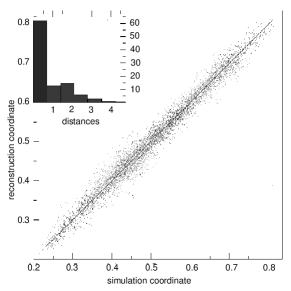
Figure 16: Test of the MAK reconstruction for a sample of $N^{\prime}=17,178$ points from a $N$-body simulation (from [25]). The scatter diagram plots reconstructed versus true initial positions. The histogram inset gives the distribution (in percentages) of distances between true and reconstructed initial positions; the horizontal unit is the distance between two sampled points. The width of the first bin is less than unity to ensure that only exactly reconstructed points fall in it. More than sixty percent of the points are exactly reconstructed.

As summarized in figure 16, the MAK reconstruction method leads to very promising results. More than 60% of the discrete points are assigned to their actual Lagrangian pre-image. Such a number has to be compared with other reconstruction methods for which the success rate barely exceed 40% for the same data set.

Even if the mapping from initial to final positions is unique, the peculiar velocities are not well defined except if we have some extra knowledge of what is happening at intermediate times $0\leq t^{\prime}\leq t$. Of course the density field $\rho(\vec{x}^{\prime},t^{\prime})$ is unknown. However, there are trivial physical requirements. First the two mass transport problems between $0$ and $t^{\prime}$ and between $t^{\prime}$ and $t$ have both to be optimal. This means that one looks for two Lagrangian maps, $\vec{X}_{1}$ from $0$ to $t^{\prime}$ and $\vec{X}_{2}$ from $t^{\prime}$ to $t$ which are minimizing the respective costs

$$\mathcal{I}_{1} = \int\|\vec{X}_{1}(\vec{x}_{0})-\vec{x}_{0}\|^{2}\rho_{0}\,\mathrm{d}^{3}x_{0},$$

$$\mathcal{I}_{2} = \int\|\vec{x}-\vec{X}_{2}^{-1}(\vec{x})\|^{2}\rho(\vec{x},t)\,\mathrm{d}^{3}x.$$ (4.41)

The second physical requirement is that the composition of these two optimal maps have to give the Lagrangian map between times $0$ and $t$, namely $\vec{X}(\vec{x}_{0},t)=\vec{X}_{2}(\vec{X}_{1})$. Under these two conditions there is equivalence between the optimal transport with a quadratic cost and the Burgers dynamics supplemented by the transport of a density field (see [13] for details).

5 Forced Burgers turbulence

5.1 Stationary régime and global minimizer

We consider in this section solutions to the forced Burgers equation. As we have seen in section 2, the solution in the limit of vanishing viscosity can be expressed at any time $t$ in terms of the initial condition at time $t_{0}$ through a variational principle which consists in minimizing an action along particle trajectories. The statistically stationary régime toward which the solution converges at large time can be studied assuming that the by rejecting the initial time $t_{0}$ is at minus infinity. The solution is then given by the variational principle

$$\Psi(\vec{x},t)\!=\!-\!\inf_{\vec{\gamma}(\cdot)}\!\left\{\int_{-\infty}^{t}\!\left[\frac{1}{2}\|\dot{\vec{\gamma}}(s)\|^{2}\!-\!F(\vec{\gamma}(s),s)\right]\!\mathrm{d}s\!\right\}\!,$$ (5.1)

where the infimum is taken over all (absolutely continuous) curves $\vec{\gamma}:(-\infty,t]\to\Omega$ such that $\vec{\gamma}(t)=\vec{x}$. In this setting, the action is computed over the whole half line $(-\infty,t]$ and the argument of the infimum does not depend anymore on the initial condition. Of course, (5.1) defines $\Psi$ up to an additive constant. This means that only the differences $\Psi(\vec{x},t)-\Psi(0,t)$ can actually be defined. A trajectory $\vec{\gamma}$ minimizing (5.1) is called a one-sided minimizer. It is easily seen from (5.1) that all the minimizers are solutions of the Euler–Lagrange equation

$$\ddot{\vec{\gamma}}(s)=-\nabla F(\vec{\gamma(s)},s)\,,$$ (5.2)

where the dots denote time derivatives. This equation defines a $2d$-dimensional (possibly random) dynamical system in the position-velocity phase space $(\vec{\gamma},\dot{\vec{\gamma}})$. The Lagrangian one-sided minimizers $\vec{\gamma}$ defined over the half-infinite interval $(-\infty,t]$ play a crucial role in the construction of the global solution and of the stationary régime. Namely, a global solution to the randomly forced inviscid Burgers equation is given by $\vec{v}(\vec{x},t)=\dot{\vec{\gamma}}(t)$ where $\vec{\gamma}(t)=\vec{x}$. To prove that such half-infinite minimizers exist, one has to take the limit $t_{0}\to-\infty$ for minimizers defined on the finite time interval $[t_{0},t]$. The existence of this limit follows from a uniform bound on the absolute value of the velocity $|\dot{\vec{\gamma}}|$ (see, e.g., [38]). Obtaining such a bound becomes the central problem for the theory, as we shall now see.

When the configuration space $\Omega$ where the solutions live is compact (bounded), one can expect the velocity of a minimizer to be uniformly bounded. Indeed, in this case the displacement of a minimizer for any time interval is then bounded by the diameter of the domain $\Omega$, so that action minimizing trajectories cannot have large velocities. For forcing potential that are delta-correlated in time, it has been shown by E et al. [38] in one dimension and by Iturriaga and Khanin [68, 69] in higher dimensions that the minimizing problem (5.1) has a unique solution $\Psi$ with the following properties:

• $\Psi$ is the unique statistically stationary solution to the Hamilton–Jacobi equation (2.2) in the inviscid limit $\nu\to 0$;

• $\Psi$ is almost everywhere differentiable with respect to the space variable $\vec{x}$;

• $-\nabla\Psi$ uniquely defines a statistically stationary solution to the Burgers equation in the inviscid limit;

• there exists a unique one-sided minimizer at those Eulerian positions $\vec{x}$ where the potential $\Psi$ is differentiable; the locations where $\Psi$ is not differentiable correspond to shocks.

• There exists a unique minimizer $\vec{\gamma}^{\rm(g)}$ that minimizes the action calculated from $-\infty$ to any time $t$. It is called the global minimizer (or two-sided minimizer) and corresponds to the trajectory of a fluid particle that is never absorbed by shocks. Moreover, all one-sided minimizers are asymptotic to it as $s\to-\infty$.

All the properties above follow from the variational approach. In fact, the variational principle (2.12) imply similar statements in the viscous case. Of course, when viscosity is positive the unique statistically stationary solution is smooth. However, one can show that the stationary distribution corresponding to such solutions converges to inviscid stationary distribution in the limit $\nu\to 0$ [58]. Although the variational proofs are conceptual, general and simple, they are based on the fluctuation mechanism and therefore do not give a good control of the rate of convergence to the statistically stationary regime. Exponential convergence would follow from the hyperbolicity of the global minimizer. Although one expects hyperbolicity holds in any dimension, mathematically it is an open problem. At present a rigorous proof of hyperbolicity is only available in dimension one [38].

The assumption of compactness of the configuration space $\Omega$ is essential in the construction of the stationary régime. As we will see in subsection 5.4, the situation is much more complex in the non-compact case when for instance the solution is defined on the whole space $\Omega={\mathbb{R}}^{d}$.

5.2 Topological shocks

To introduce the notion of topological shock we first focus on the one-dimensional case in a periodic domain, i.e. in $\Omega={\mathbb{T}}={\mathbb{R}}/{\mathbb{Z}}$. If we “unwrap” at a given time $t$ the configuration space to its universal cover ${\mathbb{R}}$ (see figure 17(a)), we then obtain an infinite number of global minimizer $\gamma^{\rm(g)}_{k}$, which at all time $s\leq t$ satisfy $\gamma^{\rm(g)}_{k+1}(s)=\gamma^{\rm(g)}_{k}(s)+1$. All the one-sided minimizers converge backward in time to one of these global minimizers. The topological shock (or main shock) is defined as the set of $x$ positions giving rise to several minimizers approaching two successive replicas of the global minimizer. This particular shock is also the only shock that has existed for all times.

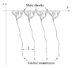
(a)

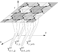
(b)

Figure 17: Space-time sketch of the unwraping of the periodic domain ${\mathbb{T}}^{d}$ to the whole space ${\mathbb{R}}^{d}$ for $d=1$ (a) and $d=2$ (b).

This construction can easily be extended to higher dimensions (see [10]). For this we unwrap the $d$-dimensional torus ${\mathbb{T}}^{d}$ to its universal cover, the full space ${\mathbb{R}}^{d}$ (see figure 17(b) for $d=2$). Then, the different replicas of the periodic domain define a lattice of global minimizers $\vec{\gamma}^{\rm(g)}_{\vec{k}}$ parameterized by integer vectors $\vec{k}$. The backward-in-time convergence on the torus of the one-sided minimizers to the global minimizer implies that a minimizer associated to a location $\vec{x}$ in ${\mathbb{R}}^{d}$ at time $t$ will be asymptotic to one of the global minimizer $\vec{\gamma}^{\rm(g)}_{\vec{k}}$ of the lattice. Hence, every position $\vec{x}$ which has a unique one-sided minimizer is associated to an integer vector $\vec{k}(\vec{x})$. This defines a tiling of space at time $t$. The tiles $\mathcal{O}_{\vec{k}}$ are the sets of points whose associated one-sided minimizers are asymptotic to the $\vec{k}$-th global minimizer. The boundaries of the $\mathcal{O}_{\vec{k}}$’s are the topological shocks. They are the locations from which at least two one-sided minimizers approach different global minimizers on the lattice. Indeed, a point where two tiles $\mathcal{O}_{\vec{k}_{1}}$ and $\mathcal{O}_{\vec{k}_{2}}$ meet, has at least two one-sided minimizers, one of which is asymptotic to $\vec{\gamma}^{(\rm g)}_{\vec{k}_{1}}$ and another to $\vec{\gamma}^{(\rm g)}_{\vec{k}_{2}}$. Of course, there are also points on the boundaries where three or more tiles meet and thus where more than two one-sided minimizers are asymptotic to different global minimizers. For $d=2$ such locations are generically isolated points corresponding to the intersections of three or more topological shock lines, while for $d=3$, they form edges and vertices where shock surfaces meet. Note that, generically, there exist other points inside $\mathcal{O}_{\vec{k}}$ with several minimizers. They correspond to shocks of “local” nature because at these locations, all the one-sided minimizers are asymptotic to the same global minimizer $\vec{\gamma}^{(\rm g)}_{\vec{k}}$ and hence, to each other. In terms of Lagrangian dynamics, the topological shocks play a role dual to that of the global minimizer. Indeed, all the fluid particles are converging backward-in-time to the global minimizer and are absorbed forward-in-time by the topological shocks. For the transportation of mass when we assume that the Burgers equation is supplemented by a continuity equation for the mass density, all the mass concentrate at large times in the topological shocks.

(a)

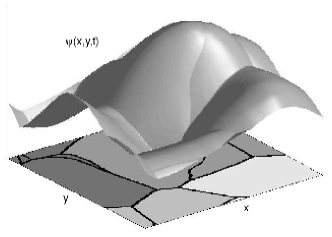
(b)

Figure 18: (a) Position of the topological shock on the torus; the two triple points are represented as dots. (b) Snapshot of the velocity potential $\psi(x,y,t)$ for $d=2$ in the statistical steady state, obtained numerically with $256^{2}$ grid points. Shock lines, corresponding to locations where $\psi$ is not differentiable, are represented as black lines on the bottom of the picture; the four gray areas are different tiles separated by the topological shocks; the other lines are local shocks.

The global structure of the topological shocks is related to the various singularities generically present in the solution to the Burgers equation that were detailed in section 2.3. Generically there are no locations associated to more than $(d+1)$ minimizers. As one expects to see only generic behavior in a random situation, the probability to have points with more than $(d+1)$ one-sided minimizers is zero. It follows that there are no points where $(d+2)$ tiles $\mathcal{O}_{\vec{k}}$ meet, which is an important restriction on the structure of the tiling. For $d=2$ it implies that the tiling is constituted of curvilinear hexagons. Indeed, suppose each tile $\mathcal{O}_{\vec{k}}$ is a curvilinear polygon with $s$ vertices corresponding to triple points. For a large piece of the tiling that consists of $N$ tiles, the total number of vertices is $n_{v}\sim sN/3$ and the total number of edges is $n_{e}\sim sN/2$. The Euler formula implies that $1=n_{v}-n_{e}+N\sim(6-s)N/6$, and we necessarily have $s=6$, corresponding to an hexagonal tiling. As shown in figure 18(a), this structure corresponds on the periodicity torus ${\mathbb{T}}^{2}$, to two triple points connected by three shock lines that are the curvilinear edges of the hexagon $O_{\vec{0}}$. The connection between the steady-state potential and the topological shocks is illustrated numerically on figure 18(b). The different tiles covering the periodic domain were obtained by tracking backward in time fluid particle trajectories and by determining to which periodic image of the global minimizer they converge.

In dimensions higher than two, the structure of topological shocks is more complicated. For instance it is not possible to determine in a unique manner the shape of the polyhedra forming the tiling. However, it has been shown by Matveev [87] that for $d=3$ the minimum polyhedra forming such tiling has 24 vertices and 36 edges and is composed of 8 hexagons and 6 rectangles (see figure 19). It is of interest to note that the structure of topological shocks is in direct relation with the notions of complexity and minimum spines of manifolds introduced by Matveev from a purely topological viewpoint.

Figure 19: Sketch of the simplest configuration of the topological shock in dimension $d=3$.

Algebraic characterization of the topological shock

In two dimensions, when periodic boundary conditions are considered, very strong constraints are imposed on the structure of the solution. In particular, the topology of the torus ${\mathbb{T}}^{2}$ imply that the topological shocks generically form a periodic tiling of ${\mathbb{R}}^{2}$ with curvilinear hexagons. However, this tiling can be of various algebraic types. Consider the tile $O_{\vec{0}}$ surrounded by its six immediate neighbors $O_{\vec{k}_{i}}$, where the integer vectors $\vec{k}_{i}$ are labeled in anti-clockwise order, $\vec{k}_{1}$ having the smallest polar angle (see figure 20). It is easily seen that the periodicity of the tiling implies

$$\vec{k}_{3}=\vec{k}_{2}-\vec{k}_{1}, \ \vec{k}_{4}=-\vec{k}_{1},\ \ \vec{k}_{5}=-\vec{k}_{2}$$ (5.3)

$$\mbox{and }\ \vec{k}_{6}=\vec{k}_{1}-\vec{k}_{2},$$

so that the whole information on the algebraic structure of the tiling is contained in the vectors $\vec{k}_{1}$ and $\vec{k}_{2}$ which form a matrix $\mathcal{S}$ from the group ${\rm SL}(2,{\mathbb{Z}})$ of $2\times 2$ integer matrices with unit determinant. The matrix $\mathcal{S}$ gives information on the number of times each shock line turns around the torus before reconnecting to another triple point. Figure 18(a) corresponds to the simplest case when $\mathcal{S}$ is the identity matrix. When the forcing is stochastic, the matrix $\mathcal{S}$ is random and stationary solutions to the two-dimensional Burgers equation define a stationary distribution on ${\rm SL}(2,{\mathbb{Z}})$.

Figure 20: The algebraic structure of the topological shock in dimension $d=2$ is determined by the indexes corresponding to immediate neighbors of the tiling considered.

Certainly, topological shocks evolve in time and may change their algebraic structure. This happens through bifurcations (or metamorphoses) described in section 2.3. In two dimensions, the generic mechanism which transforms the algebraic structure of topological shocks is the merger of two triple points. This metamorphosis is called the flipping bifurcation and corresponds to the appearance at time $t_{\star}$ of an $A_{1}^{4}$ singularity in the solution associated to a position with four minimizers. The mechanism transforming the algebraic structure of the topological shock is illustrated in figure 21. Issues such as the minimum number of flips needed to transform the matrix $\mathcal{S}_{1}$ associated to the algebraic structure of the topological shock to another matrix $\mathcal{S}_{2}$ are discussed in in [1].

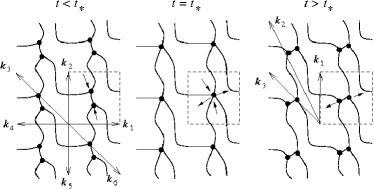
Figure 21: Sketch of the tiling before, at the flipping time $t_{*}$ and after it. This example corresponds to a bifurcation from the matrix $\mathcal{S}_{1}=[^{1}_{0}~{}^{0}_{1}]$ to $\mathcal{S}_{2}=[^{0}_{1}~{}^{-1}_{\;\;\>2}]$. The dashed boxes represent the periodicity domain $[0,1]^{2}$.

5.3 Hyperbolicity of the global minimizer

The nature of the convergence to a statistical steady state is determined by the local properties of the global minimizer. The hyperbolicity of this action-minimizing trajectory implies an exponential convergence, so that the global picture of the solution is reached very rapidly, after just a few turnover times.

Since the trajectory of the global minimizer is unique and can be extended to arbitrary large times, it corresponds to an ergodic invariant measure for the stochastic flow defined by the Euler–Lagrange equation (5.2). Conditioned by the random force, this measure is simply the delta measure sitting at the location $(\vec{\gamma}^{\rm(g)}(0),\dot{\vec{\gamma}}^{\rm(g)}(0))$. By the Oseledets ergodic theorem (see, e.g. [98]), $2d$ non-random Lyapunov exponents can be associated to the global minimizer trajectory. Since the flow is symplectic these non-random exponents come in pairs with opposite signs. That is

$$\lambda_{1}\geq\cdots\geq\lambda_{d}\geq 0\geq-\lambda_{d}\geq\cdots\geq-\lambda_{1}\,.$$ (5.4)

Hyperbolicity is defined as the non-vanishing of all these exponents. Thus, the issue of hyperbolicity can be addressed in terms of the backward-in-time convergence of the one-sided minimizers to the global one or, better, in terms of forward-in-time dynamics. In the latter case, this amounts to looking how fast Lagrangian fluid particles are absorbed by shocks. For this we consider the set $\Omega_{\rm reg}(T)$ of locations $\vec{x}$ such that the fluid particle emanating from $\vec{x}$ at time $t=0$ survives, i.e. is not absorbed by any shock, until the time $t=T$. The long-time shrinking of $\Omega_{\rm reg}$ as a function of time is asymptotically governed by the Lyapunov exponents. To ensure the absence of vanishing Lyapunov exponents, it is sufficient to show that the diameter of $\Omega_{\rm reg}(T)$ decays exponentially as $T\to+\infty$.

In one dimension, it has been shown in [38] that this is indeed the case, and particularly that there exists positive constants $\alpha$, $\beta$, $A$ and $B$ such that

$${\rm Prob}\left\{{\rm diam}\,\Omega_{\rm reg}(T)\geq A{\rm e}^{-\alpha T}\right\}\leq B{\rm e}^{-\beta T}\,.$$ (5.5)

Unfortunately this proof of hyperbolicity is purely one-dimensional and at present time there is no extension of this result to higher dimensions.

In two dimensions, the behavior of ${\rm diam}\,\Omega_{\rm reg}(T)$ at large times was studied numerically in [10] by using the fast Legendre transform described in section 2.4 and a forcing that is a sum of independent random impulses concentrated at discrete times. The ideas of this numerical method are related to the Lagrangian structure of the flow. This easily permits to track numerically the set $\Omega_{\rm reg}$ of regular Lagrangian locations. As seen from figure 22, the diameter of this set decays exponentially fast in time for three different types of forcing, providing good evidence of the hyperbolicity of the global minimizer for $d=2$.

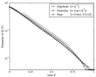
Figure 22: Time evolution of the diameter of the Lagrangian set $\Omega(T)$ (points corresponding to the regular region) for three different types of forcing spectrum; average over 100 realizations and with $256^{2}$ grid points (from [10]).

Hyperbolicity of the global minimizer implies existence at any time $t$ of two $d$-dimensional smooth manifolds in phase space $(\vec{\gamma},\dot{\vec{\gamma}})$ that are invariant by the Euler–Lagrange dynamics (5.2): a stable (attracting) manifold $\Gamma^{\rm(s)}(t)$ and an unstable (repelling) manifold $\Gamma^{\rm(u)}(t)$, defined as the instantaneous location of trajectories converging to the global minimizer forward in time and backward in time, respectively. Since all the minimizers converge backward in time to the global minimizer, the graph in the position-velocity phase space $(\vec{x},\vec{v})$ of the solution in the statistical steady state is made of pieces of the unstable manifold $\Gamma^{\rm(u)}(t)$ with discontinuities along the shocks lines or surfaces. In other words, shocks appear as jumps between two different folds of the unstable manifold. The smoothness of the unstable manifold is an important property; for instance, it implies that when $d=2$, the topological shock lines are smooth curves.

In one dimension, where hyperbolicity is ensured, the main shock corresponds to a jump between the right branch and the left branch of the unstable manifold. Its position can be obtained geometrically after observing that the area $b$ covered by the unstable manifold, once the latter is cut by the main shock, should be equal to the first integral of motion which is conserved, i.e.

$$b=\int v(x,t)\,\mathrm{d}x=\int v_{0}(x)\,\mathrm{d}x\,.$$ (5.6)

The other shocks (or secondary shocks that have existed only for a finite time) cut through the double-fold loops of the unstable manifold (see figure 23). Their locations can be obtained by a Maxwell rule applied to those loops. Indeed, the difference of the two areas defined by cutting such a loop at some position $x$ is equal to the difference of actions of the two trajectories emanating from the upper and lower locations and, thus, vanishes at the shock location. We will see in section 6 that this construction of the solution is also valid when the forcing is periodic in time, problem which can be related to Aubry–Mather theory relative to commensurate-incommensurate phase transitions.

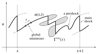
Figure 23: Sketch of the unstable manifold for $d=1$ in the $(x,v)$ plane. Shock locations ($A_{1}^{2}$ singularities) are obtained by applying Maxwell rules to the loops. A preshock ($A_{3}$ singularity) is represented; it corresponds to the formation of a loop in the manifold. The velocity profile which is the actual solution to the Burgers equation is represented as a bold line.

The above geometrical construction of the solution has much in common with that appearing in the unforced problem. Indeed, as we have seen in section 3.1, when $F=0$ the solution can be obtained geometrically by considering in the $(\vec{x},\vec{v})$ space, the Lagrangian manifold defined by the position and the velocity of the fluid particles at a given time. This analogy gives good ground predicting that some universal properties associated to the unforced problem will still hold in the forced case, as we will indeed see in section 7. Another instance concerns transport of mass in higher dimension. We have seen in section 4.1 that, for the unforced case, large but finite mass densities are localized near boundaries of shocks (“kurtoparabolic” singularities) contributing power-law tails with the exponent $-7/2$ to the probability density function of the mass density. When a force is applied the smoothness of the unstable manifold associated to the global minimizer should lead to the same universal law.

5.4 The case of extended systems

So far, we have discussed the global structure of the solution to the forced Burgers equation with periodic boundary conditions. Is is however of physical interest to understand instances when the size of the domain is much larger than the typical length scale of the forcing. In this section, we will focus on describing, in the one-dimensional case, the singular structure of the solution in unbounded domains. Based on the formalism of [11], we achieve this goal by considering a spatially periodic forcing with a characteristic scale $L_{f}$ much smaller than the system size $L$. More precisely, for a fixed size $L$ we consider the stationary régime corresponding to the limit $t\to\infty$ and then study the limit $L\to\infty$ by keeping constant the energy injection rate (i.e. the $\mathcal{L}^{2}$ norm of the forcing grows like $L$).

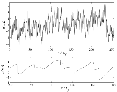
(a)

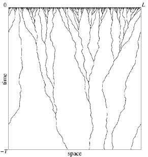
(b)

Figure 24: (a) Upper: snapshot of the velocity field for $L=256\,L_{f}$. Lower: zoom of the field in a interval of length $10\,L_{f}$. (b) Minimizing trajectories in space time for $L=256\,L_{f}$ and over a time interval of length $T=100$

In order to get an idea of the behavior of the solution, the limit of infinite aspect ration $L/L_{f}$ was investigated numerically in [11]. As seen from figure 24(a) numerical observations suggest that at any time in the statistical steady state, the shape of the velocity profile is similar to the order-unity aspect ratio problem, duplicated over independent intervals of size $L_{f}$. In particular, when tracking backward in time the trajectories of fluid particles the minimizers converge to each other in a very non-uniform way. Figure 24(b) shows that the minimizers form different branches, which are converging to each other backward in time; in space time a tree structure is obtained. As shown in figure 25(a) a similar behavior is observed for shocks.

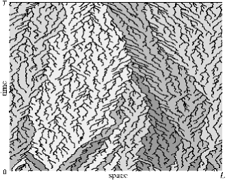
(a)

(b)

Figure 25: (a) Shock trajectories for aspect ratio $L/L_{f}=32$ and with $T=10$. The different gray areas correspond to the space-time domains associated to the different smooth pieces $\Omega_{j}$ of the velocity field at time $t=0$. (b) Sketch of the space-time evolution of a given smooth piece $\Omega_{j}$ located between two shock trajectories $X_{1}(t)$ and $X_{2}(t)$ that merge at time $T_{j}$.

The velocity field at a given time $t$, consists of smooth pieces separated by shocks. Let us denote by $\{\Omega_{j}\}$ the set of intervals in $[0,L)$, on which the solution $u(\cdot,t)$ is smooth. The boundaries of the $\Omega_{j}$’s are the shocks positions. Each of these shocks is associated to a root-like structure formed by the trajectories of the various shocks that have merged at times less than $t$ to form the shock under consideration (see figure 25(a)). This root-like structure contains the whole history of the shock and in particular its age (i.e. the length of the deeper branch of the root structure). Indeed, if the root has a finite depth, the shock considered has only existed for a finite time. A $T$-global shock is defined as a shock whose associated root is deeper than $-T$. They can alternatively be defined geometrically by considering the leftmost and the rightmost minimizer associated to it. After tracing them backward for a sufficiently long time, these two minimizers are getting close and eventually converge to each other exponentially fast (see figure 24(b)). For a $T$-global shock, the time when the two minimizers are getting within a distance smaller than the forcing correlation length $L_{f}$ is larger than $T$. As we have seen in section 5.2, the existence in one dimension of a main shock in the spatially periodic situation follows from a simple topological argument. The main shock can also be defined as the only shock that has existed forever in the past. It is hence infinitely old, contrary to all other shocks, all of them being created at a finite time and having a finite age. When the periodicity condition is dropped, the main shock disappears and it is useful to consider the $T$-global shocks that mimic the behavior of a main shock over time scales larger than $T$.

One can dually define $T$-global minimizers. All the smoothness intervals $\Omega_{j}$ defined above, except that which contains the global minimizer, will be entirely absorbed by shocks after a sufficient time (see figure 25(b)). For each of these pieces, one can define a life-time $T_{j}$ as the time when the last fluid particle contained in this piece at time $t$ enters a shock. It corresponds to the first time for which the shock located on the left of this smooth interval at time $t$ merges with the shock located on the right. When the life-time of such an interval is greater than $T$, the trajectory of the last surviving fluid particle is here called a $T$-global minimizer. Note that, when $T\to\infty$, the number of $T$-main shocks and of $T$-global minimizers is one, recovering respectively the notions of main-shock and of two-sided minimizer.

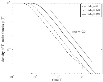
Figure 26: Density of $T$-main shocks as a function of $T$ for three different system sizes $L/L_{f}=64$, $128$ and $256$; average over 100 realizations. Lower inset: local scaling exponent.

Hence, at a given instant $t$, and for any timelag $T$, the spatial domain $[0,L)$ contains a certain number of $T$-objects. We define their spatial density as being the number of such objects, averaged with respect to the forcing realizations, divided by the size of the domain $L$. The density $\rho(T)$ of $T$-main shocks was investigated numerically in [11] for the kicked case by using a two-step method: first, the simulation was run until a large time $t$ for which the statistically stationary régime is reached; secondly, each shock present at time $t$ was tracked backward-in-time down to the instant of its creation, giving an easy way to characterize the density $\rho(T)$. It is seen in figure 26 that, for three different aspect ratios $L/L_{f}$, the density $\rho(T)$ displays a power-law behavior $\rho(T)\propto T^{-2/3}$ for the intermediate time asymptotics $L_{f}/u_{\rm rms}\ll T\ll L/u_{\rm rms}$.

We now present a simple phenomenological theory aiming to explain the scaling exponent $2/3$. We consider the solution at a fixed time ($t=0$, for instance). Denote by $\ell(T)$ the typical spatial separation scale for two nearest $T$-global shocks. Obviously, $\ell(T)\sim 1/{\rho(T)}$. The mean velocity of the spatial segment of length $\ell$ is given by

$$b_{\ell}=\frac{1}{\ell}\int_{[y,\,y+\ell]}u(x,0)\,\mathrm{d}x$$ (5.7)

Since the expected value $\langle u(x,0)\rangle=0$, and that the integral in (5.7) is over an interval of size much larger than the forcing correlation length, it is equivalent to a sum of independent centered random variables and scales as the Brownian motion. Hence, for large $\ell$ one has the following asymptotics

$$\int_{[y,\,y+\ell]}u(x,0)\,\mathrm{d}x\sim\sqrt{\ell},$$ (5.8)

which gives $b_{\ell}\sim\ell^{-1/2}$ for mean velocity fluctuations. Consider now the rightmost minimizer corresponding to the left $T$-global shock and the leftmost minimizer related to the right one. Since there are no $T$-global shocks in between, it follows that the two minimizers we selected get close to each other backward-in-time around times of the order of $-T$. This means that the backward-in-time displacement of a spatial segment of length $O(\ell)$ is itself $O(\ell)$ for time intervals of the order of $T$. The corresponding displacement is given as the sum of two competing behaviors: the first, which can be understood as a drift induced by the local mean velocity $b_{\ell}$, is due to the mean velocity fluctuations and is responsible for a displacement $\propto b_{\ell}T$; the second contribution is due to a standard diffusive scale $\propto T^{1/2}$ expressing the diffusive behavior of the minimizing trajectories. Taking into account both terms we obtain

$$\ell\sim B_{1}T\ell^{-1/2}+B_{2}T^{1/2},$$ (5.9)

where $B_{1}$ and $B_{2}$ are numerical constants. It is easy to see that the dominant contribution comes from the first term. Indeed, if the second term were to dominate, then $\ell$ would be much larger than $T$, which contradicts (5.9). Hence, one has $\ell\sim B_{1}T\ell^{-1/2}$, leading to the scaling behavior

$$\ell(T)\propto T^{2/3},\qquad\rho(T)\propto T^{-2/3}.$$ (5.10)

As we have already discussed, $T$-global shocks are shocks older than $T$. Denote by $p(A)$ the probability density function (PDF) for the age of shocks. More precisely, $p(A)$ is a density in the stationary régime of a probability distribution of the age $A(t)$ of a shock, say the nearest to the origin. It follows from (5.10) that the probability of shocks whose age is larger than $A$ decays like $A^{-2/3}$; this implies the following asymptotics for the PDF $p(A)$:

$$p(A)\propto A^{-5/3}.$$ (5.11)

Actually, the power-law behavior of the density $\rho(T)$ of $T$-global shocks can be interpreted in term of an inverse cascade in the spectrum of the solution (although there is no conserved energy-like quantity). Indeed, the fluctuations (5.8) of the mean velocity suggest that, for large-enough separations $\ell$, the velocity potential increment scales like

$$\left|\psi(x+\ell,\,t)-\psi(x,\,t)\right|\propto\ell^{1/2}.$$ (5.12)

This behavior is responsible for the presence of an intermediate power-law range with exponent $-2$ in the spectrum of the velocity potential at wavenumbers smaller than the forcing scale (see figure 27).

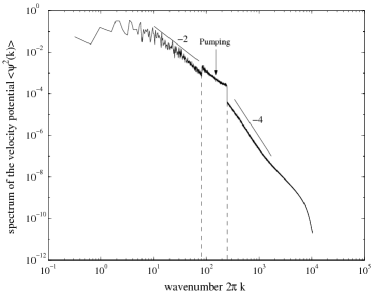
Figure 27: Spectrum $\langle\hat{\psi}^{2}(k)\rangle$ of the velocity potential in the stationary régime for the aspect ratio $L/L_{f}=128$. This spectrum contains two power-law ranges: at wavenumbers $k\gg L/L_{f}$, the traditional $\propto k^{-4}$ inertial range connected to the presence of shocks in the solution and, for $k\ll L/L_{f}$, an “inverse cascade” $\propto k^{-2}$ associated to the large-scale fluctuations of $\psi$

In order to observe the $k^{-2}$ range at small wavenumbers, the spectrum of the forcing potential must decay faster than $k^{-2}$; otherwise the leading behavior is non-universal but depends on the functional form of the forcing correlation.

The one-dimensional randomly forced Burgers equation in an unbounded domain has been studied in [66] with a different type of forcing: it was assumed that the forcing potential has at any time its global maximum and its global minimum in a prescribed compact region of space. It was proven that with these particular settings the statistically stationary régime exists and is very similar to that arising in compact domains. In particular, there exists a unique global minimizer located in a finite spatial interval for all times and all other minimizers are asymptotic to it in the limit $t\to-\infty$. The main idea behind considering such type of forcing potential is to ensure that the potential energy plays a dominant role in comparison with the kinetic (elastic) term in the action. This leads to effective compactification and allows estimates on the velocities of fluid particles. As we already mentioned in section 5.1, these estimates are very important and pave the way to the construction of the whole theory of the statistically stationary régime.

Note finally that it was shown in [76] that for special cases of forcing potentials $F(x,t)$, the velocity of a minimizers can be arbitrarily large. More specifically, one can construct pathological forcing potentials such that minimizers are accelerated and reach infinite velocities. Randomness is of course expected to prevent such a type of non-generic blow-up.

6 Time-periodic forcing

This section is devoted to the study of the solutions to the one-dimensional Burgers equation with time-periodic forcing. In this case many of the objects we have discussed above can be constructed almost explicitly: the global minimizer, the main shock etc. Also, a mathematical analysis is then much simpler. For instance, hyperbolicity of the global minimizer follows immediately from first principles. Finally, the case of time-periodic forcing is directly related to the Aubry-Mather theory as we explain below.

6.1 Kicked Burgers turbulence

We shall be concerned here with the initial-value problem for the one-dimensional Burgers equation when the force is concentrated in Dirac delta functions at discrete times:

$$f(x,t)=\sum_{j}f_{j}(x)\,\delta(t-t_{j}),$$ (6.1)

where both the “impulses” $f_{j}(x)$ and the “kicking times” $t_{j}$ are prescribed (deterministic or random). The kicking times are ordered and form a finite or infinite sequence. The impulses $f_{j}(x)$ are always taken spatially smooth, i.e. acting only at large scales. The general scheme we are presenting below holds for any sequence of impulses $f_{j}(x)$ and kicking time. Later on we shall assume that they define a time-periodic forcing. The precise meaning we ascribe to the Burgers equation with such forcing is that at time $t_{j}$, the solution $u(x,t)$ changes discontinuously by the amount $f_{j}(x)$

$$u(x,t_{j+})=u(x,t_{j-})+f_{j}(x),$$ (6.2)

while, between $t_{j+}$ and $t_{(j+1)-}$ the solution evolves according to the unforced Burgers equation.

We shall also make use of the formulation in terms of the velocity potential $\psi(x,t)$ and the force potentials $F_{j}(x)$

$$u(x,t)=-\partial_{x}\psi(x,t),\qquad f_{j}(x)=-\frac{\mathrm{d}}{\mathrm{d}x}F_{j}(x).$$ (6.3)

The velocity potential satisfies

$$\partial_{t}\psi=\frac{1}{2}(\partial_{x}\psi)^{2}+\nu\partial_{xx}\psi+\sum_{j}F_{j}(x)\,\delta(t-t_{j}),$$ (6.4)

$$\psi(x,t_{0})=\psi_{0}(x),$$ (6.5)

where $\psi_{0}(x)$ is the initial potential.

Using the variational principle we obtain the following “minimum representation” for the potential in the limit of vanishing viscosity which relates the solutions at any two times $t>t^{\prime}$ between which no force is applied:

$$\psi(x,t)=-\min_{y}\left[\frac{(x-y)^{2}}{2(t-t^{\prime})}-\psi(y,t^{\prime})\right].$$ (6.6)

As before, when $t^{\prime}$ is the initial time, the position $y$ which minimizes (6.6) is the Lagrangian coordinate associated to the Eulerian coordinate $x$. The map $y\mapsto x$ is called the Lagrangian map. By expanding the quadratic term it is easily shown that the calculation of $\psi(\cdot,t)$ from $\psi(\cdot,t^{\prime})$ is equivalent to a Legendre transformation. For details, see [104, 107].

We now turn to the forced case with impulses applied at the kicking times $t_{j}$. Let $t_{J(t)}$ be the last such time before $t$. Using (6.6) iteratively between kicks and changing the potential $\psi(y,t_{j+1})$ discontinuously by the amount $F_{j+1}(y)$ at times $t_{j+1}$, we obtain

$$\psi(x,t)=-\!\!\!\!\min_{\{y_{j}\}_{j_{0}\leq j\leq J}}\!\!\!\!\left[\mathcal{A}(\{y_{j}\};x,t;j_{0}))-\psi_{0}(y_{j_{0}})\right],$$ (6.7)

$$\mathcal{A}(\{y_{j}\};x,t;j_{0}) \equiv\frac{(x-y_{J})^{2}}{2(t-t_{J})}$$

$$+ \!\sum_{j=j_{0}}^{J-1}\left[\frac{(y_{j+1}-y_{j})^{2}}{2(t_{j+1}-t_{j})}-\!F_{j+1}(y_{j+1})\right]\!,$$ (6.8)

where $A(j_{0};x,t;\{y_{j}\})$ is called the action. We shall assume that the force potential and the initial condition are periodic in the space variable and the period is taken to be unity. This assumption is very important for the discussion below.

For a given initial condition at $t_{j_{0}}$ we next define a “minimizing sequence” associated to $(x,t)$ as a sequence of $y_{j}$’s ($j=j_{0},j_{0}+1,\ldots,J(t)$) at which the right-hand side of (6.7) achieves its minimum. Differentiating the action (6.8) with respect to the $y_{j}$’s one gets necessary conditions for such a sequence, which can be written as a sequence of (Euler–Lagrange) maps

$$v_{j+1} =v_{j}+f_{j}(y_{j}),$$ (6.9)

$$y_{j+1} =y_{j}+v_{j+1}(t_{j+1}-t_{j})$$ (6.10)

$$=y_{j}+(v_{j}+f_{j}(y_{j}))(t_{j+1}-t_{j}),$$

where

$$v_{j}\equiv\frac{y_{j}-y_{j-1}}{t_{j}-t_{j-1}}.$$ (6.11)

These equations must be supplemented by the initial and final conditions:

$$v_{j_{0}} = u_{0}(y_{j_{0}}),$$ (6.12)

$$x = y_{J}+v_{J+1}(t-t_{J}).$$ (6.13)

It is easily seen that $u(x,t)=v_{J+1}=(x-y_{J})/(t-t_{J})$. Observe that the “particle velocity” $v_{j}$ is the velocity of the fluid particle which arrives at $y_{j}$ at time $t_{j}$ and which, of course, has remained unchanged since the last kick (in Lagrangian coordinates). Equation (6.9) just expresses that the particle velocity changes by $f_{j}(y_{j})$ at the the kicking time $t_{j}$.

Note that (6.9)-(6.10) define an area-preserving and (explicitly) invertible map.

As in the case of continuous-in-time forcing we can formulate the Burgers equation in the half-infinite time interval $(-\infty,t]$ without fully specifying the initial condition $u_{0}(x)$ but only its (spatial) mean value $\left\langle u\right\rangle\equiv\int_{0}^{1}u_{0}(x)\mathrm{d}x$.

The construction of the solution in a half-infinite time interval is done by extending the concept of minimizing sequence to the case of dynamics starting at $t_{0}=-\infty$. For a half-infinite sequence $\{y_{j}\}$ ($j\leq J$), let us define the action $\mathcal{A}(\{y_{j}\};x,t;-\infty)$ by (6.8) with $j_{0}=-\infty$. Such a half-infinite sequence will be called a “minimizer” (or “one-sided minimizer”) if it minimizes this action with respect to any modification of a finite number of $y_{j}$’s. Specifically, for any other sequence $\{{\hat{y}_{j}}\}$ which coincides with $\{y_{j}\}$ except for finitely many $j$’s (i.e. ${\hat{y}_{j}}=y_{j}$, $j\leq J-k,k\geq 0$), we require

$$A(\{\hat{y}_{j}\};x,t;J-k)\geq A(\{y_{j}\};x,t;J-k).$$ (6.14)

Of course, the Euler–Lagrange relations (6.9)-(6.10) still apply to such minimizers. Hence, if for a given $x$ and $t$ we know $u(x,t)$, we can recursively construct the minimizer $\{y_{j}\}$ backwards in time by using the inverse of (6.9)-(6.10) for all $j<J$ and the final condition – now an initial condition – (6.13) with $v_{J+1}=u(x,t)$. This is well defined except where $u(x,t)$ has a shock and thus more than one value.

One way to construct minimizers is to take a sequence of initial conditions at different times $t_{0}\to-\infty$. At each such time some initial condition $u_{0}(x)$ is given with the only constraint that it have the same prescribed value for $\left\langle u\right\rangle$. Then, (finite) minimizing sequences extending from $t_{0}$ to $t$ are constructed for these different initial conditions. This sequence of minimizing sequences has limiting points (sequences themselves) which are precisely minimizers (E et al. 1998). The uniqueness of such minimizers, which would then imply the uniqueness of a solution to the Burgers equation in the time interval $]-\infty,t]$, can only be shown by using additional assumptions, for example for the case of random forcing or when the forcing is time-periodic.

If $\left\langle u\right\rangle=0$, the sequence $\{y_{j}\}$ minimizes the action $\mathcal{A}(\{y_{j}\};x,t;-\infty)$ in a stronger sense. Consider any sequence $\{{\hat{y}_{j}}\}$ such that, for some integer $P$ we have ${\hat{y}_{j}}=y_{j}+P$, $j\leq J-k,k\geq 0$ and which differs arbitrarily from $\{y_{j}\}$ for $j>J-k$. (In other words, in a sufficiently remote past the hatted sequence is just shifted by some integer multiple of the spatial period.) We then have

$$\mathcal{A}(\{\hat{y}_{j}\};x,t;-\infty)\geq\mathcal{A}(\{y_{j}\},x,t;-\infty).$$ (6.15)

Indeed, for $\left\langle u\right\rangle=0$, the velocity potential for any initial condition is itself periodic. In this case a particle can be considered as moving on the circle $S^{1}$ and its trajectory is a curve on the space-time cylinder. The $y_{j}$’s are now defined modulo 1 and can be coded on a representative $0\leq y_{j}<1$. The Euler–Lagrange map (6.9)-(6.10) is still valid provided (6.10) is defined modulo 1.

The condition of minimality implies now that $y_{j}$ and $y_{j+1}$ are connected by the shortest possible straight segment. It follows that $|v_{j+1}|=\rho(y_{j},y_{j+1})/(t_{j+1}-t_{j})$, where $\rho$ is the distance on the circle between the points $y_{j},y_{j+1}$, namely $\rho(a,b)\equiv\min\{|a-b|,1-|a-b|\}$. Hence, the action $\mathcal{A}$ can be rewritten in terms of cyclic variables:

$$\mathcal{A}(\{y_{j}\};x,t;-\infty) =\frac{\rho^{2}(x,y_{J})}{2(t-t_{J})}$$

$$+\sum_{j<J} \left[\frac{\rho^{2}(y_{j+1},y_{j})}{2(t_{j+1}-t_{j})}-F_{j+1}(y_{j+1})\right].$$ (6.16)

The concept of “global minimizers” can be defined in a usual way. Namely, global minimizers correspond to one-sided minimizers that can be continued to a bilateral sequence $\{y_{j},-\infty<j<+\infty\}$ while keeping the minimizing property. Such global minimizers correspond to trajectories of fluid particles that, from $t=-\infty$ to $t=+\infty$, have never been absorbed in a shock. As before we define a “main shock” as a shock which has always existed in the past.

From now on we shall consider exclusively the case where the kicking is periodic in both space and time. Specifically, we assume that the force in the Burgers equation is given by

$$f(x,t) = g(x)\sum_{j=-\infty}^{+\infty}\delta(t-jT),$$ (6.17)

$$g(x) \equiv -\frac{\mathrm{d}}{\mathrm{d}x}G(x),$$ (6.18)

where $G(x)$, the kicking potential, is a deterministic function of $x$ which is periodic and sufficiently smooth (e.g. analytic) and where $T$ is the kicking period. The initial potential $\psi_{\rm init}(x)$ is also assumed smooth and periodic. This implies that the initial velocity integrates to zero over the period. The case where this assumption is relaxed will be considered later in connection with the Aubry–Mather theory.

The numerical experiments of [9] reported here have been made with the kicking potential

$$G(x)=\frac{1}{3}\sin 3x+\cos x,$$ (6.19)

and a kicking period $T\!=\!1$. Other experiments were done with (i) $G(x)=-\cos x$ and (ii) $G(x)=(1/2)\cos(2x)-\cos x$. The former potential produces a single shock and no preshock. As a consequence it displays no $-7/2$ law in the PDF of gradients. The latter potential gives essentially the same results as reported hereafter but has an additional symmetry. To avoid non-generic behaviors that could result from this symmetry, it was chosen to focus on the forcing potential given by (6.19).

The number of collocation points chosen for such simulations was mostly $N_{x}=2^{17}\approx 1.31\times 10^{5}$, with a few simulations done at $N_{x}=2^{20}$ (for the study of the relaxation to the periodic régime presented below). Since the numerical method allows going directly to the desired output time (from the nearest kicking time) there is no need to specify a numerical time step. However, in order to perform temporal averages, e.g. when calculating PDF’s or structure functions, without missing the most relevant events (which can be sharply localized in time) sufficiently frequent temporal sampling is needed. The total number of output times $N_{t}\approx 1000$, is thus chosen such that the increment between successive output times is roughly the two-thirds power of the mesh (this is related to the cubic structure of preshocks, see section 2.3).

Figure 28 shows snapshots of the time-periodic solution at various instants.

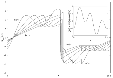
Figure 28: Snapshots of the velocity for the unique time-periodic solution corresponding to the kicking force $g(x)$ shown in the upper inset; the various graphs correspond to six output times equally spaced during one period. The origin of time is taken at a kick. Notice that during each period, two new shocks are born and two mergers occur. (From [9].)

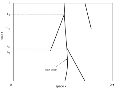
Figure 29: Evolution of shock positions during one period. The beginnings of lines correspond to births of shocks (preshocks) at times $t_{\star 1}$ and $t_{\star 2}$; shock mergers take place at times $t_{c1}$ and $t_{c2}$. The “main shock”, which survives for all time, is shown with a thicker line.

It is seen that shocks are always present (at least two) and that at each period two new shocks are born at $t_{\star 1}\approx 0.39$ and $t_{\star 2}\approx 0.67$. There is one main shock which remains near $x=\pi$ and which collides with the newborn shocks at $t_{c1}\approx 0.44$ and $t_{c2}\approx 0.86$. Figure 29 shows the evolution of the positions of shocks during one period.

It was found that, for all initial conditions $u_{0}(x)$ used, the solution $u(x,t)$ relaxes exponentially in time to a unique function $u_{\infty}(x,t)$ of period 1 in time. Figure 30 shows the variation of $\int_{0}^{2\pi}|u(x,n_{-})-u_{\infty}(x,1_{-})|\,\mathrm{d}x/(2\pi)$ for three different initial conditions as a function of the discrete time $n$.

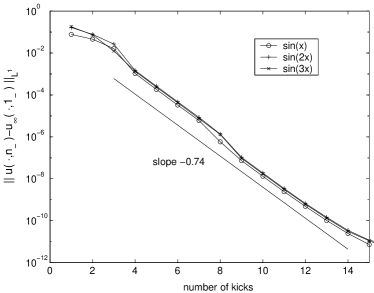
Figure 30: Exponential relaxation to a time-periodic solution for three different initial velocity data as labeled. The horizontal axis gives the time elapsed since $t=0$. (From [9].)

The phenomenon of exponential convergence to a unique space- and time-periodic solution is something quite general: whenever the kicking potential $G(x)$ is periodic and analytic and the initial velocity potential is periodic (so that the mean velocity $\left\langle u\right\rangle$ =0 at all times), there is exponential convergence to a unique piecewise analytic solution. This can be proved rigorously (see Appendix to [9]) in the case when the functions $G(x)$ have a unique point of maximum with a non-vanishing second derivative (Morse generic functions). Here, we just explain the main ideas of the proof and give some additional properties of the unique solution.

One very elementary property of solutions is that, for any initial condition of zero mean value, the solution after at least one kick satisfies

$$|u(x,t)|\leq(1/2)+\max_{x}|\mathrm{d}G(x)/\mathrm{d}x|.$$ (6.20)

Indeed, at a time $t=n_{-}$ just before any kick we have $x=y+u(x,n_{-})$ where $y$ is the position just after the previous kick of the fluid particle which goes to $x$ at time $n_{-}$. It follows from the spatial periodicity of the velocity potential that the location $y$ which minimizes the action is within less than half a period from $x$. Thus, $|u(x,n_{-})|\leq 1/2$. The additional $\max_{x}|\mathrm{d}G(x)/\mathrm{d}x|$ term comes from the maximum change in velocity from one kick. Hence the solution is bounded. Note that if the spatial and temporal periods are $L$ and $T$, respectively, the bound on the velocity becomes $L/(2T)+\max_{x}|\mathrm{d}G(x)/\mathrm{d}x|$.

The convergence at large times to a unique solution can be understood in terms of the two-dimensional conservative (area-preserving) dynamical system defined by the Euler–Lagrange map (6.9)-(6.10). By construction, we have $u(x,1_{+})=\hat{u}(x)-\mathrm{d}G(x)/\mathrm{d}x$, where $\hat{u}(x)$ is the solution of the unforced Burgers equation at time $t=1_{-}$ from the initial condition $u(x)$ at time $t=0_{+}$. The map $u\mapsto\hat{u}(x)+g(x)$, where $g(x)\equiv-\mathrm{d}G(x)/\mathrm{d}x$, here denoted $B_{g}$, solves the kicked Burgers equation over a time interval one. The problem is to show that the iterates $B_{g}^{n}u_{0}$ converge as $n\to\infty$ to a unique solution.

If it were not for the shocks it would suffice to consider the two-dimensional Euler–Lagrange map. Note that, for the case of periodic kicking, this map has an obvious fixed point $P$, namely $(x=x_{c},v=0)$, where $x_{c}$ is the unique point maximizing the kicking potential. It is easily checked that this fixed point is an unstable (hyperbolic) saddle point of the Euler–Lagrange map with two eigenvalues $\lambda=1+c+\sqrt{c^{2}+2c}$ and $1/\lambda$, where $c=-\partial^{2}_{xx}G(x_{c})/2$.

(a)

(b)

Figure 31: (a) Sketch of a hyperbolic fixed point $P$ with stable ($\Gamma^{\rm(s)}$) and unstable ($\Gamma^{\rm(u)}$) manifolds. The dashed line gives the orbit of successive iterates of a point near the stable manifold. (b) Unstable manifold $\Gamma^{\rm(u)}$ on the $(x,v)$-cylinder (the $x$-coordinate is defined modulo 1) which passes through the fixed point $P=(x_{c},0)$. The bold line is the graph of $u_{\infty}(x,1_{-})$. The main shock is located at $x_{l}=x_{r}$. Another shock at $x_{1}$ corresponds to a local zig-zag of $\Gamma^{\rm(u)}$ between A and B.

Like for any two-dimensional map with a hyperbolic fixed point, there are two curves globally invariant by the map which intersect at the fixed point. The first is the stable manifold $\Gamma^{\rm(s)}$, i.e. the set of points which converge to the fixed point under indefinite iteration of the map; the second is the unstable manifold $\Gamma^{\rm(u)}$, i.e. the set of points which converge to the fixed point under indefinite iteration of the inverse map, as illustrated in figure 31(a). Any curve which intersects the stable manifold transversally (at the intersection point, the two curves are not tangent to each other) will, after repeated applications of the map, be pushed exponentially against the unstable manifold at a rate determined by the eigenvalue $1/\lambda$. In the language of Burgers dynamics, the curve in the $(x,v)$ plane defined by an initial condition $u_{0}(x)$ will be mapped after time $n$ into a curve very close to the unstable manifold. In fact, for the case studied numerically, $1/\lambda\approx 0.18$ is within one percent of the value measured from the exponential part of the graph shown in figure 30. Note that if the initial condition $u_{0}(x)$ contains the fixed point, the convergence rate becomes $\left(1/\lambda\right)^{2}$ (even higher powers of $1/\lambda$ are possible if the initial condition is tangent to the unstable manifold).

The fixed point $P$ is actually a very simple global minimizer: $(y_{j}=x_{c},\,v_{j}=0)$ for all positive and negative $j$’s. It follows indeed by inspection of (6.16) that any deviation from this minimizer can only increase the action; actually, this trajectory minimizes both the kinetic and the potential part of the action. Note that the corresponding fluid particle is at rest forever and will never be captured by a shock (it is actually the only particle with this property). It is easy to see that any minimizer is attracted exponentially to such a global minimizer as $t\to-\infty$. Thus, any point $(y_{j},v_{j})$ on a minimizer belongs to the unstable manifold $\Gamma^{\rm(u)}$ and, hence, any regular part of the graph of the limiting solution $u_{\infty}(x)$ belongs to the unstable manifold $\Gamma^{\rm(u)}$. This unstable manifold is analytic but can be quite complicated. It can have several branches for a given $x$ (see figure 31(b)) and does not by itself define a single-valued function $u_{\infty}(x)$. The solution has shocks and is only piecewise analytic. Consideration of the minimizers is required to find the position of the shocks in the limiting solution: two points with the same $x$ corresponding to a shock, such as A and B on figure 31(b) should have the same action.

Figure 32: Minimizers (trajectories of fluid particles) on the $(x,t)$-cylinder. Time starts at $-\infty$. Shock locations at $t=0_{-}$ are characterized by the presence of two minimizers (an instance is at $x_{1}$). The main shock is at $x_{l}=x_{r}$. The fat line $x=x_{c}$ is the global minimizer.

Finally, we give the geometric construction of the main shock, the only shock which exists for an infinite time. Since the eigenvalue $\lambda$ is positive, locally, minimizers which start to the right of $x_{c}$ approach the global minimizer from the right, and those which start to the left approach it from the left. Take the rightmost and leftmost points $x_{r}$ and $x_{l}$ on the periodicity interval such that the corresponding minimizers approach the global minimizer from the right and left respectively (see figure 32). These points are actually identical since there cannot be any gap between them that would have minimizers approaching the global minimizer neither from the right nor the left. The solution $u_{\infty}(x)$ has then its main shock at $x_{l}=x_{r}$.

6.2 Connections with Aubry–Mather theory

In the previous subsection, the study of the solutions to the periodically kicked Burgers equation was limited to initial conditions with a vanishing spatial average $b$. With a non-vanishing mean velocity $b$, which in the forced case cannot be eliminated by a Galilean invariance, many of the properties of the solutions described above are still valid. However the action now depends on $b$. Global minimizers $\{y_{j}^{\rm(g)},\,j\in{\mathbb{Z}}\}$ exist in this case as well. However generically they are not unique and do not correspond to fixed points of the Euler–Lagrange map (6.9)-(6.10). A global minimizer now minimizes the action

$$\mathcal{A}_{\infty}(\{y_{k}\}) = \mathcal{A}(\{y_{k}\};+\infty;-\infty)$$ (6.21)

$$= \!\!\sum_{k=-\infty}^{+\infty}\!\!\left[\frac{1}{2T}(y_{k+1}\!-\!y_{k}\!-\!b)^{2}\!\!-\!G(y_{k+1})\right]\!.$$

This action is exactly the potential energy associated to an infinite chain of atoms linked by elastic springs and embedded in a periodic potential, problem known as the Frenkel–Kontorova model [52]. The parameter $b$ represents the equilibrium length $l$ of the springs and the spatial period $L$ of the external potential (see figure 33) is equal to 1.

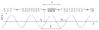
Figure 33: Sketch of the Frenkel–Kontorova model for the equilibrium states of an atom chain in a periodic potential.

A global minimizer of (6.21) represents an equilibrium configuration of this system. The properties of this equilibrium, or ground states are determined by the competition between two tendencies: on the one hand the atoms tend to stabilize at those locations where the potential is minimum; on the other hand, the springs tend to maintain them at a fixed distance of each other. When $b=0$ this competition disappears and the equilibrium is given by $y_{k}=x_{c}$, where $x_{c}$ is the location at which $G$ attains its global minimum. For $b\neq 0$, the situation is more delicate and the structure of the ground states involves, as we shall now see, a problem of commensurate-incommensurate transition. The properties of ground states were studied in great details by Aubry [3] and Mather [86].

The relations between the Burgers equation with a time-periodic forcing and Aubry–Mather theory were discussed for the first time in [70] and in [38]. The theory was further developed in [36, 106]. For integer values of $b$, the global minimizer is trivially associated to the fixed point $(x,v)=(x_{c},b)$ of the Euler–Lagrange map (6.9)-(6.10), which corresponds to a fluid trajectory located at integer times at $x=x_{c}$ and which moves on distance of $b$ spatial periods during one temporal period. A similar argument implies that it is enough to study values of $b$ in the interval $[0,1)$.To each global minimizer $\{y_{j}^{\rm(g)},\,j\in{\mathbb{Z}}\}$ is associated a rotation number defined as

$$\rho\equiv\lim_{J\to\infty}\frac{1}{J}\sum_{j=0}^{J}\left(y_{j+1}^{\rm(g)}-y_{j}^{\rm(g)}\right)\,,$$ (6.22)

which represents the time-average velocity of the minimizer. For a fixed value of the spatial average $b$ of the velocity, all global minimizers associated to the solution of the Burgers equation have the same rotation number $\rho$. Indeed, as the dynamics is restricted to a compact domain of the configuration space (in our case ${\mathbb{T}}$), two minimizers with different rotation numbers necessarily cross each other; this is an obvious obstruction to the action minimization property. In the case of rational rotation numbers the global minimizers correspond to periodic orbits of the dynamical system defined by the Euler–Lagrange map. An important feature is that for rational $\rho$, the rotation number does not change when varying $b$ over a certain closed interval $[b_{\min},b_{\max}]$, called the mode-locking interval. On the contrary, irrational $\rho$ correspond to a unique value of the parameter $b$. Such “irrational” values of $b$ form a Cantor set of zero Lebesgue measure. In particular, the graph of $\rho$ as a function of the parameter $b$ is a “Devil staircase” (see figure 34).

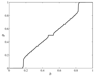
Figure 34: Rotation number $\rho$ as a function of the spatial mean of the velocity $b$ for the standard map.

When $\rho$ is rational ($\rho=p/q$ in irreducible form), global minimizers correspond to a periodic orbit of period $q$. It is easy to see that such an orbit generates $q$ different but closely related global minimizers. Of course each of these global minimizer is the image of another one by the Euler–Lagrange map and is mapped back to itself after $q$ iterations. This procedure generates a periodic orbit, which turns out to be hyperbolic one. Hence, each of the $q$ global minimizers has a one-dimensional unstable manifold associated to it. The solution to the Burgers equation is formed by branches of these various manifolds with jumps between them defining $q$ global shocks.

The picture is very different for values of $b$ corresponding to irrational rotation numbers. Consider velocities and positions of all global minimizers at a fixed moment of time, say $t=0$. They form a subset $\mathcal{G}$ of the phase space ${\mathbb{T}}\times{\mathbb{R}}$. Then two cases have to be distinguished:

• The set $\mathcal{G}$ forms a closed invariant curve for the Euler–Lagrange map. This invariant curve has a one-to-one projection onto the base ${\mathbb{T}}$ and dynamics on the curve is conjugated to a rigid rotation by angle $\rho$. The limiting solution of the Burgers equation is given by the invariant curve and does not contain any shocks.

• The set $\mathcal{G}$ forms an invariant Cantor set and the limiting solution of the Burgers equation contains an infinite number of shocks, none of which is a main shock.

The Kolmogorov [80], Arnold [2] and Moser [93] theory (frequently referred to as KAM) describes invariant curves (or invariant tori) for small analytic perturbations of integrable Hamiltonian systems, and thus the various types of dynamical trajectories. The KAM theory ensures that for sufficiently small perturbations, most of the invariant curves associated to Diophantine irrational rotation numbers are stable with respect to small analytic perturbations of the system. Diophantine irrational numbers possess fast converging approximations by rational numbers (in a suitable technical sense). However, these invariant curves may disappear from the perturbed system when an interaction corresponding to a non-integrable perturbation gets sufficiently strong. Aubry–Mather theory provides another variational description for the KAM invariant curves. But even more importantly, it describes the invariant Cantor sets that appear instead of invariant curves in the case of strong nonlinear interactions. We have mentioned already that these Cantor sets correspond to global minimizers. Thus Aubry–Mather theory provides information about the global minimizers and, hence, allows one to study in such a situation the properties of limiting entropic solutions and, in particular, the structure of shocks.

A numerical study of the Burgers equation in the inviscid limit, with periodic forcing and a non-vanishing spatial average of the velocity, reveals the appearance of shock accumulations. Such events occur for the values of the mean velocity $b$ near the end-points of the mode-locking intervals, corresponding to rational rotation numbers. The shock accumulation phenomenon is due to the fact that the end-points $b_{\min},b_{\max}$ of the mode-locking intervals can be approximated by convergent sequences of “irrational” values of the parameter $b$. This implies accumulation of shocks, since for irrational rotation numbers the number of shocks is infinite.

The limiting solution $u_{\infty}(x,t)$ is completely determined by the function $\hat{u}(x)$ defined in the previous subsection. The function $\hat{u}(x)$ corresponds to a stroboscopic section of $u_{\infty}$ right after each impulse. The regular parts of $\hat{u}$ are made of single-valued functions related to the unstable manifolds. The shocks correspond to jumps, either between different branches of the same manifold (secondary shocks), or between the manifolds associated to different global minimizers (main shocks).

When the rotation number is rational ($\rho=p/q$), there are $q$ global minimizers. The positions of the $q$ main shocks of $\hat{u}$ are determined by a requirement that the area defined by the graph of the solution is equal to the conserved quantity $b$. The latter constraint shows that the values of $b$ compatible with the rotation number $p/q$ belong to an interval $[b_{\min},b_{\max}]$ bounded by the minimum and maximum areas defined by the unstable manifolds, as illustrated in figure 35.

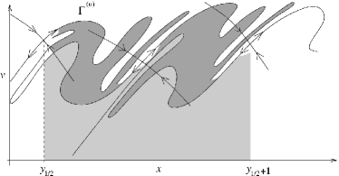
Figure 35: Sketch of the unstable manifolds of the two global minimizers associated to the rotation number $\rho=1/2$. The values $b_{\min}$ and $b_{\max}$ given by this configurations are represented as grey areas.

The detailed shape of the manifolds can actually not be sketched on a figure. Generically the unstable manifold of a global minimizer corresponding to a particular point of the basic periodic orbit of period $q$ intersects transversally with the stable manifold of another minimizer corresponding to another point of the periodic orbit. Such an intersection leads to formation of a heteroclinic tangle, a notion which can be traced back to the work of Poincaré. The heteroclinic intersection results in the formation of an infinite number of zig-zags of the unstable manifolds. These zig-zags are accumulating along the stable manifold and come arbitrary close to the corresponding point of the periodic orbit. The zig-zags contract exponentially in one direction (along the stable manifold) and are stretched exponentially in the other direction. It is easy to see that the accumulation of zig-zags generates an infinite number of “potential” shocks of smaller and smaller size which also accumulate near the periodic orbit. When the parameter $b$ is located well inside the mode-locking interval, the position of the main shock cuts off the accumulated shocks of small size so that the total number of shocks is of the order of unity. However, when $b$ gets closer and closer to $b_{\max}$ or $b_{\min}$, the main shocks move closer to the periodic points and a larger number of the small accumulating shocks appears in the solution. This mechanism leads to an infinite number of shocks in the solution when $b$ is equal to $b_{min}$ or $b_{\max}$ (see figure 36(a)).

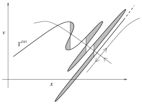
(a)

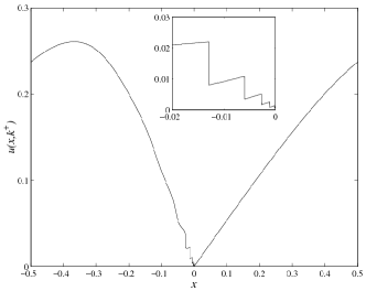
(b)

Figure 36: (a) Accumulations of shocks occurring for $b=b_{\min}$ or $b=b_{\max}$, due to the presence of an infinite number of loops of the unstable manifold in the homocline or heterocline tangle. (b) Shock accumulation at the fixed point $(0,0)$ of the standard map. Here, $\lambda=0.1$ and $b=0.15915$. The latter value is close to the upper bound of the interval associated to $\rho=0$. The upper inset is a zoom near $(0,0)$, illustrating the accumulation of shocks.

Both the distances between two consecutive shocks and the sizes of the shocks decrease exponentially fast with the number of shocks; the rate is given by the stable eigenvalue associated to the hyperbolic periodic orbit. It is interesting to mention that when $b=b_{min}$ or $b=b_{max}$ the main shocks merge with the periodic orbit associated to the global minimizers. Hence, for the end-points of the mode-locking interval the main shocks disappear.

To illustrate numerically the change in behavior of the solution to the Burgers equation when the mean velocity $b$ changes, we focus here on the simple periodic kicking potential $G(x)=(\lambda/2\pi)\,\cos(2\pi x)$ where $\lambda$ is a free parameter. The associated Euler–Lagrange map then reads

$$\mathcal{T}\!\!:(y,v)\!\mapsto\!\left(y\!+\!v\!+\!\lambda\sin(2\pi y),v\!+\!\lambda\sin(2\pi y)\right)\!.$$ (6.23)

This transformation is usually called the standard map (or Chirikov–Taylor map). It is one of the simplest model for studying the presence of chaos in Hamiltonian dynamical systems and in particular particularly to study the KAM theory.

Figure 36(b) illustrates the accumulation of shocks due to the homoclinic or heteroclinic tangling for the first transition (starting from $b=0$). This transition corresponds to a rotation number of the global minimizer changing value from $\rho=0$ to $\rho>0$. When $b$ is increased and gets close to the critical value, shocks accumulate on the left-hand side of the global minimizer located at $(y,v)=(0,0)$.

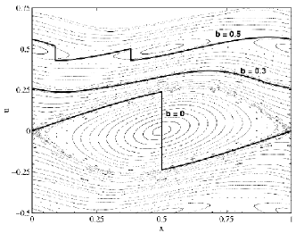
(a)

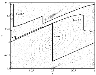
(b)

Figure 37: General aspect in position-velocity phase space of the dynamical system defined by the standard map (6.23) for two different values of the parameter (a) $\lambda=0.1$ and (b) $\lambda=0.3$. The corresponding time-periodic solutions to the kicked Burgers equation are represented as bold lines in both cases. The results are presented for the spatial mean velocities $b=0$, $b=0.3$ and $b=0.5$.

Other numerical experiments were performed in order to observe the destruction of invariant curves and the accumulation of shocks on Cantor sets for irrational rotation numbers. It is of course impossible numerically to set the rotation number to an irrational value. Indeed, the values of $b$ for which $\rho$ is irrational are in a Cantor set. It is however possible to be very close to irrational rotation numbers. Figure 37 illustrates the changes in the behavior of the solutions to the periodically kicked Burgers equation when varying the parameter $\lambda$. The time-asymptotic solutions associated to various values of the mean velocity $b$ are shown for $\lambda=0.1$ and $\lambda=0.3$. For the latter value, all KAM invariant curves have already disappeared. For $b=0$ and for all values of $\lambda$ the global minimizer trivially corresponds to the fixed point $(0,0)$ with a vanishing rotation number. For $b=0.5$ there are two global minimizers associated to the rational rotation number $\rho=1/2$. For $\lambda=0.1$ and $b=0.3$ the rotation number is much closer to an irrational than in previous cases. The solution is then very close to the invariant curve associated to this value. Note that the main shock is actually located close to $x\approx 0.85$. It is so small that it can hardly be seen. When $\lambda=0.3$ the value $b=0.3$ of the mean velocity no more corresponds to a rotation number close to an irrational value; it is now in the mode-locking interval associated to $\rho=1/3$. This change in the rotation number reflects the dependence of the mode-locking intervals $[b_{\min},b_{\max}]$ on the parameter $\lambda$. The interval of values of $b$ associated to $\rho=0$ is represented as a function of $\lambda$ in figure 38. Such a structure is frequently called an Arnold tongue (see, e.g., [72]).

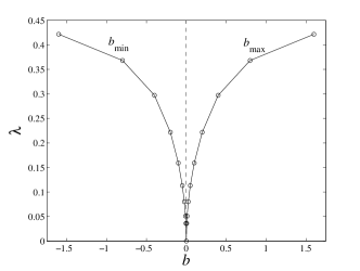
Figure 38: Evolution as a function of the parameter $\lambda$ of the mode-locking interval $[b_{\min},b_{\max}]$ associated to the rotation number $\rho=0$. Such a graph is frequently referred to as an Arnold tongue.

Finally, we discuss the structure of shocks in the case when the global minimizers form a Cantor set. There are then infinitely many gaps with no global minimizers. It is known in this case that all the gaps can be split into the finite number of images of the main gaps. For the standard map there is only one main gap. Its end-points $(x^{1},v^{1})$ and $(x^{2},v^{2})$ belong to the Cantor set associated to the global minimizers. All other gaps can be obtained by iterating this main gap with the Euler-Lagrange map (Standard map) for both positive and negative times: $(x^{1}_{i},v^{1}_{i})=\mathcal{T}^{i}(x^{1},v^{1}),\,(x^{2}_{i},v^{2}_{i})=\mathcal{T}^{i}(x^{2},v^{2}),\,i\in{\mathbb{Z}}$. One can show that the length of the $i$th gap tends to zero as $i\to\pm\infty$. Since global minimizers are hyperbolic trajectories one can connect the end-points of the main gap by two smooth curves: the stable manifold $\Gamma^{\rm(s)}$ and the unstable manifold $\Gamma^{(\rm u)}$. As $i\to\infty$ the iterates of the stable manifold $\mathcal{T}^{i}\Gamma^{(\rm s)}$ tend to a straight segment connecting the $i$-th gap with end-points at $(x^{1}_{i},v^{1}_{i})$ and $(x^{2}_{i},v^{2}_{i})$. The same is true for iterates of the unstable manifold $\mathcal{T}^{i}\Gamma^{(\rm u)}$ in the limit $i\to-\infty$. On the contrary, negative iterates of the stable manifold and positive of the unstable one form exponentially long curves connecting corresponding gaps. As usual we are interested in the iterates of the unstable manifold since they appear in the time-periodic solution of the Burgers equation. Such a solution is formed by the iterates of the unstable manifold connecting all the gaps. Note that in the case of large negative $i$, the unstable manifold is close to a straight segment; hence there are no shocks located inside the corresponding gaps. Conversely, for large positive $i$, the unstable manifold is exponentially long and possesses large zig-zags. Hence, the solution to the Burgers equation has one or several shocks inside such gaps. Since there are no shocks for gaps with large enough negative $i$, it follows that all the shocks have a finite age. In other words, the time-periodic solution has no main shocks.

At the moment it was not possible to study numerically the strange behavior of the solutions to the Burgers equation corresponding to global minimizers living on Cantor-like sets. Looking for such cases requires a very high spatial resolution in order to minimize the numerical error in the approximation of the solution. Moreover, a large number of values for the parameters $b$ and $\lambda$ has to be investigated in order to observe such a phenomenon. This would require heavy computer ressources. However, many other aspects of the Aubry–Mather theory for Hamiltonian systems can be studied numerically using the Burgers equation with periodic kicks. For instance it could be very useful for analyzing the higher dimensional versions.

7 Velocity statistics in randomly forced Burgers turbulence

The universality of small-scale properties in fully developed Navier–Stokes turbulence has frequently been investigated, assuming that a steady state is maintained by an external large-scale forcing. It is generally conjectured that the velocity increments have universal statistical properties with respect to such a force. Understanding this issue in simpler models of turbulence has motivated much work for over ten years. A toy model which has been extensively studied is the passive transport of a scalar field by random flows (see, e.g., [46]). Tools borrowed from statistical physics and field theory were used to describe and explain the anomalous scaling laws observed in the scalar spatial distribution. It was shown that the scale invariance symmetry is broken by geometrical constraints on tracer configurations that are statistically conserved by the dynamics. Universality of the intermittent scaling exponents with respect to the forcing was proven for the case where energy is injected at large scales [31, 57, 103, 14].

Issues of universality for the nonlinear Burgers turbulence model has also been very much on the focus. The possibility to solve exactly a hydrodynamical problem displaying the same kind of quadratic nonlinearity as Navier–Stokes turbulence constitutes of course the central motivation. Three independent approaches were published almost simultaneously in 1995 and were at the origin of the growing interest in Burgers turbulence. First, an analogy was made in [22] between forced Burgers turbulence and the problem of a directed polymer in a random medium. This analogy was used to show that the shocks appearing in the solution lead to anomalous scaling laws for the structure functions. The strong intermittency could be related to the replica-symmetry-breaking nature of the disordered system associated to Burgers turbulence. This approach is discussed in subsection 7.1. Second, ideas using operator product expansions borrowed from quantum field theory were proposed in [99]. The goal was to close in the inertial range the equations governing the correlations of the velocity field in one dimension. This treatment of the dissipative anomaly is described in subsection 7.2. It yields a prediction for the probability density function (PDF) of velocity increments and gradients and in particular to a power-law behavior for the PDF of $\partial_{x}v$ at large negative values [99]. However, the value of the exponent of this algebraic tail has been a matter of controversy. An overview of the various works related to this issue is given in subsection 7.3. Finally, the turbulent model of the one-dimensional Burgers equation with a self-similar forcing was proposed in [30] as one of the simplest nonlinear hydrodynamical problem displaying multiscaling of the velocity structure function. As stressed in subsection 7.4 this problem is easily tractable numerically and some of the numerical observations can be confirmed by a one-loop renormalization group expansion.

In what follows we consider the solutions to the Burgers equation with a homogeneous Gaussian random forcing that is delta-correlated in time. Namely, the spatio-temporal correlation of the forcing potential is taken to be

$$\left\langle F(\vec{x},t)\,F(\vec{x}^{\prime},{t}^{\prime})\right\rangle=B(\vec{x}-\vec{x}^{\prime})\,\delta(t-{t}^{\prime})\,.$$ (7.1)

The function $B$ contains information on the spatial structure of the forcing. It can be either smooth (i.e. concentrated at large spatial scales) or asymptotically self-similar (i.e. behaving as a power law at small separations). In the former case the solution reaches exponentially fast a statistically stationary régime in any space dimension. The construction of the solution in this régime in terms of global minimizer and main shock is described in detail in section 5. When $B$ does not decrease sufficiently fast at small separations (e.g. $B(r)\sim r^{2h}$ with $h<1$ as $r\to 0$ in one dimension), there is no rigorous proof of the existence of a statistically stationary régime. However we assume in the sequel that such a stationary régime exists in order to perform a statistical analysis of the solutions to Burgers equation.

7.1 Shocks and bifractality – a replica variational approach

The replica solution for Burgers turbulence proposed in [22] is based on its analogy with the problem of a directed polymer in a random medium. As already stated in the Introduction, the viscous Burgers equation forced by the potential $F$ is equivalent to finding the partition function $\mathcal{Z}$ of an elastic string in the quenched spatio-temporal disorder $V(\vec{x},t)\!=\!F(\vec{x},t)/2\nu$ (remember that $t$ has to be interpreted as the space direction in which the polymer is oriented). This relation is obtained by applying to the velocity potential $\Psi$ the Hopf–Cole transformation $\mathcal{Z}(\vec{x},t)\!=\!\exp(\Psi(\vec{x},t)/2\nu)$. The solution of the problem can be written in terms of the path integral

$$\mathcal{Z}(\vec{x},t)=\displaystyle\int_{\vec{\gamma}(t)=\vec{x}}\exp(-\mathcal{H}(\vec{\gamma}))\,\,\mathrm{d}[\vec{\gamma}(\cdot)]\,,$$

$$\mbox{with }\displaystyle\mathcal{H}(\vec{\gamma})=\frac{1}{2\nu}\int_{-\infty}^{t}\left[\left\|\dot{\vec{\gamma}}(s)\right\|^{2}+F(\vec{\gamma}(s),s)\right]\mathrm{d}s.$$ (7.2)

In the analogy between Burgers turbulence and directed polymers, the polymer temperature is assumed to be unity and its elastic modulus is $1/(2\nu)$. The strength of the potential fluctuations applied to the polymer depends on the viscosity and is $\propto\varepsilon^{1/2}L_{f}/(2\nu)$ (where $\varepsilon$ is the energy injection rate and $L_{f}$ is the spatial scale of forcing). In order to calculate the various moments of the velocity field $\vec{v}=-\nabla\Psi$, one needs to average the logarithm of the partition function $\mathcal{Z}$, a celebrated problem in disordered systems.

Bouchaud, Mézard and Parisi proposed in [22] the use of a replica trick in order to estimate the average free energy $\langle\ln\mathcal{Z}\rangle$. The first step is to write the zero-replica limit $\ln\mathcal{Z}=\lim_{n\to 0}\,(\mathcal{Z}^{n}-1)/n$. Then, the moments $\langle\mathcal{Z}^{n}\rangle$ are used to generate an effective attraction between replicas: they are written as the partition functions of the disorder-averaged Hamiltonian $\mathcal{H}_{n}(\vec{\gamma}_{1},\dots,\vec{\gamma}_{n})$ associated to $n$ replicas of the same system [90]

$$\mathcal{H}_{n}\!=\!\!\sum_{i=1}^{n}\!\!\int_{-\infty}^{t}\!\!\!\!\!\!\!\mathrm{d}s\!\!\left[\!\frac{1}{2\nu}\!\left\|\dot{\vec{\gamma}}_{i}(s)\!\right\|^{2}\!\!\!\!-\!\frac{1}{4\nu^{2}}\!\!\sum_{j=1}^{n}\!B(\vec{\gamma}_{i}(s)\!-\!\vec{\gamma}_{j}(s))\!\right]\!\!,$$ (7.3)

where $B$ denotes the spatial part of the forcing potential correlation. The next step is to study this problem by a variational approach. The Hamiltonian $\mathcal{H}_{n}$ is replaced by an effective Gaussian quadratic Hamiltonian that can be written as

$$\mathcal{H}_{\rm eff}\!=\!\frac{1}{2}\!\sum_{i=1}^{n}\sum_{j=1}^{n}\!\!\int_{-\infty}^{t}\!\int_{-\infty}^{t}\!\!\!\!\!\!\vec{{\gamma}}_{i}(\tau)\mathcal{G}_{ij}(\tau\!-\!\tau^{\prime})\vec{{\gamma}}_{j}(\tau^{\prime})\mathrm{d}\tau\mathrm{d}\tau^{\prime}\!.$$ (7.4)

The kernel $\mathcal{G}_{ij}$ is then chosen in such a way that it minimizes the free energy. It is shown in [22] that the optimal Gaussian Hamiltonian is the solution of a system of equations that can be solved following the ansatz proposed in [89]. When $d>2$ this approach singles out two régimes depending on the Reynolds number $\mbox{\it Re}=\varepsilon^{1/3}L_{f}^{3/4}/\nu$. These régimes are separated by the critical value $\mbox{\it Re}_{c}=[2(1-2/d)^{1-d/2}]^{1/3}$. When $\mbox{\it Re}<\mbox{\it Re}_{c}$ the optimal solution is of the form $\mathcal{G}_{ij}=\mathcal{G}_{0}\,\delta_{ij}+\mathcal{G}_{1}$ and obeys the replica symmetry. In finite-size systems it corresponds to a linear velocity profile. When $\mbox{\it Re}>\mbox{\it Re}_{c}$ the correct solution is given by the one-step replica-symmetry-breaking scheme (see [89]). The off-diagonal elements of $\mathcal{G}_{ij}$ are then parameterized with two functions depending on whether the indices $i$ and $j$ belong to the same block or to different blocks. Qualitatively, the one-step replica-symmetry-breaking approach amounts to the assumption that the instantaneous velocity potential can be written as a weighted sum of Gaussians, leading to an approximation of the velocity field as

$$\vec{v}(\vec{x},t)\simeq\frac{2\nu}{\sigma}\,\frac{\sum_{\alpha}(\vec{x}-\vec{r}_{\alpha})\,{\rm e}^{-\mbox{\scriptsize\it Re}\,(f_{\alpha}+\|\vec{x}-\vec{r}_{\alpha}\|^{2}/2L_{f}^{2})}}{\sum_{\alpha}{\rm e}^{-\mbox{\scriptsize\it Re}\,(f_{\alpha}+\|\vec{x}-\vec{r}_{\alpha}\|^{2}/2L_{f}^{2})}}\,,$$ (7.5)

where the $f_{\alpha}$’s are independent variables with a Poisson distribution of density $\exp(-f)$. The $\vec{r}_{\alpha}$ are uniformly and independently distributed in space. In (7.5) the sum over $\alpha$ is running from 1 to a large-enough integer $M$. The typical shape of the approximation of the velocity field given by (7.5) is represented in figure 39(a) in the two-dimensional case. In the limit of large Reynolds numbers the random velocity field given by (7.5) typically contains cells of width $\propto L_{f}$. The width of a shock separating two cells is of the order of $L_{f}/\mbox{\it Re}$.

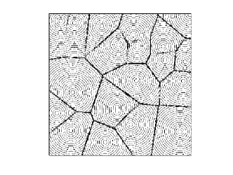
(a)

(b)

Figure 39: (a) Typical shape of the velocity field given by the replica approximation in dimension $d=2$ obtained from (7.5) for $\mbox{\it Re}=10^{3}$. The contour lines represent the velocity modulus. Note the cell structure of the domain. (b) Scaling exponents of the $p$th order structure function.

The replica approximation (7.5) leads to an estimate of the PDF $p(\Delta v,r)$ of the longitudinal velocity increment $\Delta v=(\vec{v}(\vec{x}+r\,\vec{e},t)-\vec{v}(\vec{x},t))\cdot\vec{e}$, where $\vec{e}$ is an arbitrary unitary vector. When $\mbox{\it Re}\gg 1$ and $r\ll L_{f}$ this approximation takes the particularly simple asymptotic form

$$p(\Delta v,r)\approx\delta\!\left(\Delta v-U_{f}\frac{r}{L_{f}}\right)+\frac{r}{L_{f}}\,\frac{1}{U_{f}}\,g\left(\frac{\Delta v}{U_{f}}\right)\,,$$ (7.6)

where $U_{f}=\mbox{\it Re}\,\nu/L_{f}$ is the typical velocity associated to the scale $L_{f}$ and $g$ is a scaling function that is determined explicitly in [22]. This approximation is in agreement with the following qualitative picture. With a probability almost equal to one, the two points $\vec{x}$ and $\vec{x}+r\,\vec{e}$ lie in the same cell; the velocity increment is then given by the typical velocity gradient which, according to the approximation (7.5), is order $U_{f}/L_{f}$. With a probability $r/L_{f}$ the two points are sitting on different sides of a shock separating two such cells and the associated velocity difference is of the order of $U_{f}$.

The structure functions of the velocity field given by the various moments of $\Delta v$ can be straightforwardly estimated from the approximation (7.6). Their scaling behavior $\langle\Delta v^{p}\rangle\sim r^{\zeta_{p}}$ at small separations $r$ display a bifractal behavior as sketched in figure 39(b). When $p<1$, the first term on the right-hand side of (7.6) dominates and $\langle\Delta v^{p}\rangle\propto U_{f}^{p}\,(r/L_{f})^{p}$. For $p>1$ the shock contribution is dominating the small-$r$ behavior and thus $\langle\Delta v^{p}\rangle\propto U_{f}^{p}\,(r/L_{f})$.

This approach, which makes use of replica tricks, is as we have seen able to catch the leading scaling behavior of velocity structure functions in any dimension. It is based on approximations of the velocity field by the superposition (7.5) of Gaussian velocity potentials. A first advantage of this method is that it catches the generic aspect of the solution including the hierarchy of high-order singularities appearing in the solution when $\mbox{\it Re}\to\infty$ which was examined in section 2.3. This method also gives predictions regarding the dependence on Re of the statistical properties of the solution. However, as stressed in [22], the validity of this approximation is expected to hold only in the limit of infinite space dimension $d$. In particular, it is known that for $d\leq 2$ a full continuous replica-symmetry-breaking scheme is needed [89]. Nevertheless, as we have seen, there is enough evidence that this approach describes very well the qualitative aspects of the solution.

7.2 Dissipative anomaly and operator product expansion

The replica-trick approach described in the previous subsection cannot reproduce one of the main statistical features of the solution, namely the tails of the velocity increments PDF $p(\Delta v,r)$. Indeed the prediction (7.6) based on a variational approximation of the velocity field implies that $p$ identically vanishes when $\Delta v>U_{f}\,(r/L_{f})$. In order to study the quantitative behavior of the PDF $p(\Delta v,r)$ in the inviscid limit $\nu\to 0$ (or equivalently $\mbox{\it Re}\to\infty$), Polyakov [99] proposed to use an operator product expansion. This approach leads to an explicit expression for $p(\Delta v,r)$ and predicts a super-exponential tail at large positive values and a power-law behavior for negative ones. Such predictions have immediate implications for the asymptotics of the PDF $p(\xi)$ of the velocity gradient $\xi=\partial_{x}v$. The work of Polyakov was the starting point of a controversy on the value of the exponent of the left tail of $p(\xi)$. Before returning to this issue in the next subsection, we give in the sequel a quick overview of the original work by Polyakov.

We henceforth focus on the one-dimensional solutions to the Burgers equation with Gaussian forcing whose autocorrelation is given by (7.1). Following [99] (see also [19, 20]) we introduce the characteristic function of the $n$-point velocity distribution

$$Z_{n}(\lambda_{j},x_{j};t)\equiv\left\langle{\rm e}\,^{\lambda_{1}\,v(x_{1},t)+\cdots+\lambda_{n}\,v(x_{n},t)}\right\rangle\,.$$ (7.7)

For a finite value of the viscosity $\nu$, it is easily seen that this quantity is a solution to a Fokker–Planck (master) equation obtained by differentiating $Z_{n}$ with respect to $t$ and using the Burgers equation and the fact that the forcing is Gaussian and $\delta$-correlated in time. This leads to

$$\frac{\partial Z_{n}}{\partial t} + \sum_{j}\lambda_{j}\,\frac{\partial}{\partial\lambda_{j}}\left(\frac{1}{\lambda_{j}}\,\frac{\partial Z_{n}}{\partial x_{j}}\right)=$$ (7.8)

$$= \frac{1}{2}\sum_{i,j}b(x_{i}-x_{j})\,\lambda_{i}\,\lambda_{j}\,Z_{n}+\mathcal{D}^{(n)}_{\nu}\,,$$

where $b\equiv(\mathrm{d}^{2}B)/(\mathrm{d}r^{2})$ denotes the spatial part of the correlation of the forcing applied to the velocity field. $\mathcal{D}^{(n)}_{\nu}$ denotes the contribution of the dissipative term and reads

$$\mathcal{D}^{(n)}_{\nu}\equiv\nu\,\left\langle\!\left[\sum_{j}\lambda_{j}\,\partial_{x_{j}}^{2}v(x_{j},t)\right]\!{\rm e}^{\sum_{j}\lambda_{j}\,v(x_{j},t)}\right\rangle\!.$$ (7.9)

This term does not vanish in the limit $\nu\to 0$ since the solutions to the Burgers equation develop singularities with a finite dissipation. It has been proposed in [99] to use an analogy with the anomalies appearing in quantum field theory in order to tackle this term in the inviscid limit. The important assumption is then made that the singular term in the operator product expansion relates linearly to the characteristic function $Z_{n}$. Since this expansion should preserve the statistical symmetries of the Burgers equation, it leads to the replacement in all averages of the singular limit $\lim_{\nu\to 0}\nu\,\lambda\,(\partial_{x}^{2}v)\,{\rm e}^{\lambda\,v}$ by the asymptotic expression

$$\left(\frac{\mathsf{a}}{2}+\frac{\mathsf{b}-1}{\lambda}\,\frac{\partial}{\partial x}+\mathsf{c}\,\lambda\,\frac{\partial}{\partial\lambda}\right){\rm e}^{\lambda\,v}\,,$$ (7.10)

where the coefficients $\mathsf{a}$, $\mathsf{b}$ and $\mathsf{c}$ are parameters that can be determined only indirectly. However their possible values can be restricted by requiring that $Z_{n}$ is the characteristic function of a probability distribution which is non-negative, finite, normalizable, and that the dissipative term $\mathcal{D}^{(n)}_{\nu}$ acts as a positive operator. Finding these coefficients is similar to an eigenvalue problem in quantum mechanics.

We now come to a crucial point in Polyakov’s approach. Important restrictions on the form of the different anomalous terms in (7.10) result from the fact that the solutions to the Burgers equation obey a certain form of Galilean invariance. A notion of “strong Galilean principle” is introduced for invariance of the $n$-point distribution of velocity under the transformation $v\mapsto v+v_{0}$ with $v_{0}$ an arbitrary constant. As a consequence, the $n$-point characteristic function $Z_{n}$ has to be proportional to $\delta(\lambda_{1}+\cdots+\lambda_{n})$. The operators appearing in the limit $\nu\to 0$ have to be consistent with such an invariance. In [99] it is argued that this symmetry is automatically broken by the forcing that introduces a typical velocity $\langle v^{2}\rangle^{1/2}\propto b^{1/3}(0)\,L^{1/3}$. However Polyakov assumes this “strong Galilean principle” to be asymptotically recovered in the limit $L\to\infty$ of infinite-size systems. In the case of finite-size systems, when $L$ is of the order of the correlation length $L_{f}$ of the forcing, the strong Galilean symmetry is broken because of the conservation of the spatial average of $v$ which introduces a characteristic velocity $v_{0}=(1/L)\int v(x,t)\,\mathrm{d}x$. However, the Galilean symmetry should be recovered when averaging the correlation functions with respect to the mean velocity $v_{0}$. This symmetry restoration was introduced in [20] where it is referred to as the “weak Galilean principle”. The $n$-point characteristic function associated to an average velocity $v_{0}$ relates to that associated to a vanishing mean velocity by

$$Z_{n}(\lambda_{j},x_{j};t;v_{0})={\rm e}^{v_{0}\sum_{j}\lambda_{j}}\,Z_{n}(\lambda_{j},x_{j};t;0)\,.$$

After averaging with respect to $v_{0}$, one obtains

$$Z_{n}(\lambda_{j},x_{j};t)=2\pi\,\delta\!\!\left(\sum_{j}\lambda_{j}\right)\,Z_{n}(\lambda_{j},x_{j};t;0)\,.$$ (7.11)

One can easily check that (7.8), together with the dissipative term given by (7.10), are compatible with this expression for the $n$-point characteristic function $Z_{n}$. Moreover, any higher-order term in the expansion (7.10) of the dissipative anomaly would violate Galilean invariance.

To obtain the statistical properties of the solution, one needs to further restrict the values of the three free parameters $\mathsf{a}$, $\mathsf{b}$, and $\mathsf{c}$ appearing in the expansion (7.10). Following [99] this can be done by considering the case $n=2$ that corresponds to the equation for the PDF of velocity differences. Performing the change of variables $\lambda_{1,2}=\Lambda\pm\mu$ and $x_{1,2}=X\pm y/2$, and assuming that $\lambda\ll\mu$ and $y\ll L_{f}$ (so that the spatial part of the forcing correlation is to leading order $b(y)\simeq b_{0}-b_{1}y^{2}$), the stationary and space-homogeneous solutions to the master equation (7.8)) satisfy

$$\frac{\partial^{2}Z_{2}}{\partial\mu\partial y} - (2b_{0}\Lambda^{2}+b_{1}\mu^{2}y^{2})Z_{2}=$$ (7.12)

$$= \mathsf{a}Z_{2}+\frac{2\mathsf{b}}{\mu}\frac{\partial Z_{2}}{\partial y}+\mathsf{c}\Lambda\frac{\partial Z_{2}}{\partial\Lambda}+\mathsf{c}\mu\frac{\partial Z_{2}}{\partial\mu}\,.$$

It is next assumed in [99] (see also [20]) that the velocity difference $v(x_{1},t)-v(x_{2},t)$ is statistically independent of the mean velocity $(v(x_{1},t)+v(x_{2},t))/2$. This implies that the two-point characteristic function factorizes as $Z_{2}=Z_{2}^{+}(\Lambda)Z_{2}^{-}(\mu,y)$, where the two functions $Z_{2}^{+}$ and $Z_{2}^{-}$ satisfy the closed equations

$$-2b_{0}\Lambda^{2}Z_{2}^{+} = \mathsf{c}\Lambda\frac{\partial Z_{2}^{+}}{\partial\Lambda}\,,$$ (7.13)

$$\frac{\partial^{2}Z_{2}^{-}}{\partial\mu\partial y}-b_{1}\mu^{2}y^{2}Z_{2}^{-} = \mathsf{a}Z_{2}^{-}+\frac{2\mathsf{b}}{\mu}\frac{\partial Z_{2}^{-}}{\partial y}+\mathsf{c}\mu\frac{\partial Z_{2}^{-}}{\partial\mu}\,.$$ (7.14)

The solution to the first equation corresponds to a Gaussian distribution which is normalizable only if $\mathsf{c}<0$. As shown numerically in [20] this distribution is representative of the bulk of the one-point velocity PDF. Information on the solutions to the second equation can be obtained assuming the scaling property $Z_{2}^{-}(\mu,y)=\Phi(\mu y)$, which amounts to considering only those contributions to the distribution of velocity differences stemming from velocity gradients $\xi=\partial_{x}v$. This yields a prediction the negative and positive tails of the PDF of velocity gradients:

$$p(\xi)\propto|\xi|^{-\alpha}\ \mbox{ when }\xi\to-\infty\,,$$ (7.15)

$$p(\xi)\propto\xi^{\beta}\exp(-\mathsf{C}\,\xi^{3})\ \mbox{ when }\xi\to+\infty\,,$$ (7.16)

where $\mathsf{C}$ is a constant, which depends only on the strength of the forcing. The two exponents $\alpha$ and $\beta$ are related to the coefficient $\mathsf{b}$ of the anomaly by

$$\alpha=2\mathsf{b}+1\mbox{ and }\beta=2\mathsf{b}-1\,.$$ (7.17)

The value of $\mathsf{b}$ remains undetermined but is prescribed to belong to a certain range. This approach was first designed in [99] for infinite-size systems where strong Galilean invariance holds. In that case consistency with such an invariance leads to dropping the third term in the operator product expansion (i.e. $\mathsf{c}=0$). Positivity and normalizability of the two-point velocity PDF and non-positivity of the anomalous dissipation operator imply that the two other coefficients form a one-parameter family with $3/4\leq\mathsf{b}\leq 1$. In particular, this implies that the left tail of the velocity gradient PDF with exponent $\alpha$ should be shallower than $\xi^{-3}$. As we will see in the next section, strong evidence has been obtained that $p(\xi)\propto\xi^{-7/2}$ for $\xi\to-\infty$. This seems to contradict the approach based on operator product expansion. However, as argued in [20], the breaking of strong Galilean invariance occurring in finite-size systems and resulting in the presence of the $\mathsf{c}$ anomaly broadens the range of admissible values for $\mathsf{b}$. In particular it allows for the value $\mathsf{b}=5/4$ which corresponds to the exponent $\alpha=7/2$.

7.3 Tails of the velocity gradient PDF

After the numerical work of Chekhlov and Yakhot [29], the asymptotic behavior at large positive and negative values of the PDF of velocity derivatives $\xi=\partial_{x}v$ for the one-dimensional randomly forced Burgers equation attracted much attention. A broad consensus emerged around the prediction of Polyakov [99] that $p(\xi)$ displays tails of the form (7.16) and (7.15), but the values of the exponents $\alpha$ and $\beta$ were at the center of a controversy. Note that the presence of a super-exponential tail $\propto\exp(-\mathsf{C}\,\xi^{3})$ at large positive arguments has been confirmed by the use of instanton techniques [60] and that the only remaining uncertainty concerns the exponent of the algebraic prefactor. A standard approach to determine the exponents $\alpha$ and $\beta$ appearing in (7.15) and (7.16) makes use of the stationary solutions to the inviscid limit of the Fokker–Planck equation for the PDF, namely

$$-\partial_{\xi}\left(\xi^{2}p\right)-\xi p+\nu\partial_{\xi}\left[\left\langle\partial_{x}^{3}v\,|\,\partial_{x}v\!=\!\xi\right\rangle p\right]=\tilde{b}\partial_{\xi}^{2}p\,.$$ (7.18)

Here the brackets $\left\langle\cdot|\cdot\right\rangle$ denote conditional averages and the right-hand side expresses the diffusion of probability due to the delta-correlation in time of the forcing. The main difficulty in studying the solutions of (7.18) stems from the treatment of the dissipative term $D^{\nu}(\xi)=\nu\partial_{\xi}\left[\left\langle\partial_{x}^{3}v|\partial_{x}v\!=\!\xi\right\rangle p\right]$ in the limit $\nu\to 0$. The value $\alpha=3$ is obtained if a piecewise linear approximation is made for the solutions of the Burgers equation [21]. Gotoh and Kraichnan [59] argued that the dissipative term is to leading order negligible and presented analytical and numerical arguments in favor of $\alpha=3$ and $\beta=1$. However, the inviscid limit of (7.18) contains anomalies due to the singular behavior of $D^{\nu}(\xi)$ in the limit $\nu\to 0$. As we have seen in previous section, the approach based on the use of an operator product expansion [99] leads to a relation involving unknown coefficients which must be determined, e.g., from numerical simulations [111, 19, 20], and restricts the possible values to $5/2\leq\alpha\leq 3$ [6]. Anomalies cannot be studied without a complete description of the singularities of the solutions, such as shocks, and a thorough understanding of their statistical properties.

E, Khanin, Mazel and Sinai made a crucial observation in [37] that large negative gradients stem mainly from preshocks, that is the cubic-root singularities in the velocity preceding the formation of shocks (see section 2.3). They then used a simple argument for determining the fraction of space-time where the velocity gradient is less than some large negative value. This leads to $\alpha=7/2$, provided preshocks do not cluster. Later on, this approach has been refined by E and Vanden Eijnden who proposed to determine the dissipative anomaly of (7.18) using formal matched asymptotics [39] or bounded variation calculus [42]. As we shall see below, with the assumption that shocks are born with a zero amplitude, that their strengths add up during collisions, and that there ar no accumulations of preshocks, the value $\alpha=7/2$ was confirmed [42]. Other attempts to derive this value using also isolated preshocks have been made [81, 6]. Note that there are simpler instances, including time-periodic forcing [9] (see section 6) and decaying Burgers turbulence with smooth random initial conditions [8, 42] (see section 4.1), which fall in the universality class $\alpha=7/2$, as can be shown by systematic asymptotic expansions using a Lagrangian approach.

We give here the flavor of the approach used in [39] in order to estimate the dissipative anomaly $D^{0}(\xi)=\lim_{\nu\to 0}D^{\nu}(\xi)$. One first notices that for $|\xi|\gg\tilde{b}^{1/3}$, the forcing term in the right-hand side of (7.18) becomes negligible, so that stationary solutions to the Fokker–Planck equation satisfy

$$p(\xi)\approx|\xi|^{-3}\int_{-\infty}^{\xi}\!\!\mathrm{d}\xi^{\prime}\,\xi^{\prime}D^{\nu}(\xi^{\prime}).$$ (7.19)

A straightforward consequence of this asymptotic expression is that, if the integral in the right-hand side decreases as $\xi\to-\infty$ (i.e. if $\xi D^{\nu}(\xi)$ is integrable), then $p(\xi)$ decreases faster than $|\xi|^{-3}$, and thus $\alpha>3$.

To get some insight into the behavior of $D^{\nu}$ as $\nu\to 0$, one next observes that the solutions to the one-dimensional Burgers equation contain smooth regions where viscosity is negligible, which are separated by thin shock layers where dissipation takes place. The basic idea consists in splitting the velocity field $v$ into the sum of an outer solution away from shocks and of an inner solution near them for which boundary layer theory applies. Matched asymptotics are then used to construct a uniform approximation of $v$. To construct the inner solution near a shock centered at $x=x_{\star}$, one performs the change of variable $x\mapsto\tilde{x}=(x\!-\!x_{\star})/\nu$ and looks for an expression of $\tilde{v}(\tilde{x},t)=v(x_{\star}\!+\!\nu\tilde{x},t)$ in the form of a Taylor expansion in powers of $\nu$: $\tilde{v}=\tilde{v}_{0}+\nu\tilde{v}_{1}+\mathrm{o}(\nu)$. At leading order, the inner solution satisfies

$$\left[\tilde{v}_{0}-v_{\star}\right]\partial_{\tilde{x}}\tilde{v}_{0}=\partial^{2}_{\tilde{x}}\tilde{v}_{0},$$ (7.20)

where $v_{\star}=(\mathrm{d}x_{\star})/(\mathrm{d}t)$. This expression leads to the well-known hyperbolic tangent velocity profile

$$\tilde{v}_{0}=v_{\star}-\frac{s}{2}\tanh\!\left(\frac{s\tilde{x}}{4}\right).$$ (7.21)

Here, $s=v(x_{\star}+,t)-v(x_{\star}-,t)$ denotes here the velocity jump across the shock and is given by matching conditions to the outer solution. The term of order $\nu$ is then a solution of

$$\partial_{t}\tilde{v}_{0}+\left[\tilde{v}_{0}-v_{\star}\right]\partial_{\tilde{x}}\tilde{v}_{1}=\partial^{2}_{\tilde{x}}\tilde{v}_{1}+f(x,t).$$ (7.22)

In order to evaluate the dissipative anomaly, it is convenient to assume spatial ergodicity so that the viscous term in (7.18) can be written as

$$D^{\nu}(\xi)=\nu\partial_{\xi}\!\lim_{L\to\infty}\frac{1}{2L}\int_{-L}^{L}\!\!\mathrm{d}x\,\,\partial_{x}^{3}v\,\,\delta(\partial_{x}v\!-\!\xi).$$ (7.23)

In the limit $\nu\to 0$ the only remaining contribution stems from shocks and is thus given by the inner solution. Using the expansion of the solution up to the first order in $\nu$, this leads to writing the dissipative term in the limit of vanishing viscosity as (see Appendix of [41] for details)

$$D^{0}(\xi)=\frac{\rho}{2}\int_{-\infty}^{0}\!\!\!\mathrm{d}s\,s\,[p^{+}(s,\xi)+p^{-}(s,\xi)]\,,$$ (7.24)

where $\rho$ is the density of shocks and $p^{+}$ (respectively $p^{-}$) is the joint probability of the shock jump and of the value of the velocity gradient at the right (respectively left) of the shock. This expression guarantees the finiteness of the dissipative anomaly, and in particular the fact that the integral in the right-hand side of (7.19) is finite in the limit $\nu\to 0$ and converges to 0. As a consequence, this gives a proof that the exponent $\alpha$ of the left tail of the velocity gradient PDF is larger than $3$.

To proceed further, E and Vanden Eijnden proposed to estimate the probability densities $p^{+}$ and $p^{-}$ by deriving master equations for the joint probability of the shock strength $s$, its velocity $v_{\star}$ and the values $\xi^{\pm}$ of the velocity gradient at its left and at its right. This is done in [42] using a formulation of Burgers dynamics stemming from bounded variation calculus. More precisely, it is shown in [108] that the Burgers equation is equivalent to considering the solutions to the partial differential equation

$$\partial_{t}v+\bar{v}\partial_{x}v=f\,,$$ (7.25)

where $\bar{v}(x,t)=(v(x+,t)+v(x-,t))/2$. Basically this means that Burgers dynamics can be formulated in terms of the transport of the velocity field by its average $\bar{v}$. This formulation straightforwardly yields a master equation for $v(x\pm,t)$ and $\partial_{x}v(x\pm,t)$ which is then used to estimate $p^{\pm}$ and the dissipative anomaly (7.24). Although the treatment of the master equation does not involve any closure hypothesis, it is not fully rigorous: in particular it requires the assumption that shocks are created with zero amplitude and that shock amplitudes add up during collision. However such an approaches strongly suggests that $\alpha=7/2$ and $\beta=1$.

Obtaining numerically clean scaling for the PDF of gradients is not easy with standard schemes. Let us observe that any method involving a small viscosity, either introduced explicitly (e.g. in a spectral calculation) or stemming from discretization (e.g. in a finite difference calculation), may lead to the presence of a power-law range with exponent $-1$ at very large negative gradients [59]. This behavior makes the inviscid $|\xi|^{-\alpha}$ range appear shallower than it actually is, unless extremely high spatial resolution is used. In contrast, methods that directly capture the inviscid limit with the appropriate shock conditions, such as the fast Legendre transform method [94], lead to delicate interpolation problems. They have been overcome in the case of time-periodic forcing [9] but with white-noise-in-time forcing, it is difficult to prevent spurious accumulations of preshocks leading to $\alpha=3$.

To avoid such pitfalls, a Lagrangian particle and shock tracking method was developed in [6]. This method is able to separate shocks and smooth parts of the solution and is particularly effective for identifying preshocks. The main idea is to consider the evolution of a set of $N$ massless point particles accelerated by a discrete-in-time approximation of the forcing with a uniform time step. When two of these particles intersect, they merge and create a new type of particle, a shock, characterized by its velocity (half sum of the right and left velocities of merging particles) and its amplitude. The particle-like shocks then evolve as ordinary particles, capture further intersecting particles and may merge with other shocks. In order not to run out of particles too quickly, the initial small region where particles have the least chance of being subsequently captured is determined by localization of the global minimizer of the Lagrangian action (see section 5.1). The calculation is then restarted from $t=0$ for the same realization of forcing but with a vastly increased number of particles in that region. This particle and shock tracking method gives complete control over shocks and preshocks.

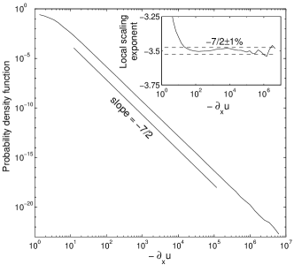
Figure 40: PDF of the velocity gradient at negative values in log-log coordinates obtained by averaging over 20 realizations and a time interval of 5 units of time (after relaxation of transients). The simulation involves up to $N=10^{5}$ particles and the forcing is applied at discrete times separated by $\delta t=10^{-4}$. Upper inset: local scaling exponent (from  [6]).

Figure 40 shows the PDF of the velocity gradients in log-log coordinates at negative values, for a Gaussian forcing restricted to the first three Fourier modes with equal variances such that the large-scale turnover time is order unity. Quantitative information about the value of the exponent is obtained by measuring the “local scaling exponent”, i.e. the logarithmic derivative of the PDF calculated in this case using least-square fits on half-decades. It is seen that over about five decades, the local exponent is within less than 1% of the value $\alpha=7/2$ predicted by E et al. [37].

7.4 Self-similar forcing and multiscaling

As we have seen in section 7.1, the solutions to the Burgers equation in a finite domain and with a large-scale forcing have structure functions (moments of the velocity increment) displaying a bifractal scaling behavior. Such a property can be easily interpreted by the presence of a finite number of shocks with a size order unity in the finite system. Somehow this double scaling and its relationship with singularities gives some insight on the multiscaling properties that are expected in the case of turbulent incompressible hydrodynamics flows. There is a general consensus that the turbulent solutions to the Navier–Stokes equations display a full multifractal spectrum of singularities which are responsible for a nonlinear $p$-dependence of the scaling exponents $\zeta_{p}$ associated to the scaling behavior of the $p$-th order structure function [53]. The construction of simple tractable models which are able to reproduce such a behavior has motivated much work during the last decades. Significant progress, both analytical and numerical, has been made in confirming multiscaling in passive-scalar and passive-vector problems (see, e.g., [46] for a review). However, the linearity of the passive-scalar and passive-vector equations is a crucial ingredient of these studies, so it is not clear how they can be generalized to fluid turbulence and the Navier–Stokes equation.

After the work of Chekhlov and Yakhot [30], it appeared that the Burgers equation with self-similar forcing could be the simplest nonlinear partial differential equation which has the potential to display multiscaling of velocity structure functions. We report in this section various works that tried to confirm or to weaken this statement. Let us consider the solutions to the one-dimensional Burgers equation with a forcing term $f(x,t)$ which is random, space-periodic, Gaussian and whose spatial Fourier transform has correlation

$$\langle{\hat{f}}(k,t){\hat{f}}(k^{\prime},t^{\prime})\rangle=2D_{0}\,|k|^{\beta}\,\delta(t-t^{\prime})\,\delta(k+k^{\prime}).$$ (7.26)

The exponent $\beta$ determines the scaling properties of the forcing. When $\beta>0$ the force acts at small scales; for instance $\beta=2$ corresponds to thermal noise for the velocity potential, and thus to the KPZ model for interface growth [74]. It is well known in this case (see, e.g., [5]) that the solution displays simple scaling (usually known as KPZ scaling), such that $\zeta_{q}=q$ for all $q$. More generally, the case $\beta>0$ can be exactly solved using a one-loop renormalization group approach [88].

As stressed in [64], renormalization group techniques fail when $\beta<0$ and the forcing acts mostly at large scales and non-linear terms play a crucial role. When $\beta<-3$, the forcing is differentiable in the space variable, the solution is piecewise smooth and contains a finite number of shocks with sizes order unity. The scaling exponents are then $\zeta_{p}=\min\,(1,\,p)$. In the case of non-differentiable forcing ($-3<\beta<0$), the presence of order-unity shocks and dimensional arguments suggest that the scaling exponents are $\zeta_{p}=\min\,(1,\,-p\beta/3)$. However, very little is known regarding the distribution of shocks with intermediate sizes. In particular, there is no clear evidence whether or not they form a self-similar structure at small scales. We summarize here some studies which were done on Burgers turbulence with self-similar forcing to show how difficult it might be to measure scaling laws of structure functions and in particular how logarithmic corrections can masquerade anomalous scaling.

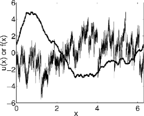
Figure 41: Representative snapshots of the velocity $v$ (jagged line) in the statistically stationary régime, and of the integral of the force $f$ over a time step (rescaled for plotting purposes).

For this we focus on the case $\beta=-1$ which has attracted much attention; indeed, dimensional analysis suggests that $\zeta_{p}=p/3$ when $p\leq 3$, leading to a K41-type $-5/3$ energy spectrum. Early studies [29, 30] seemed to confirm this prediction using pseudo-spectral viscous numerical simulations at rather low resolutions (around ten thousands gridpoints). It was moreover argued in [64, 65] that a self-similar forcing with $-1<\beta<0$, could lead to genuine multifractality. The lack of accuracy in the determination of the scaling exponents left open the question of a weak anomalous deviation from the dimensional prediction. This question was recently revisited in [91] with high-resolution inviscid numerical simulations using the fast Legendre transform algorithm (see section 2.4.2). A typical snapshot of the forcing and of the solution in the stationary régime are represented in figure 41. It is clear that because of shocks the velocity develops small-scale fluctuations much stronger than those present in the force. However one notices that shock dynamics and spatial finiteness of the system lead, as predicted, to the presence of few shocks with order-unity sizes.

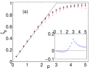
Figure 42: Scaling exponents $\zeta_{p}$ versus order $p$ for $N=2^{16}(\diamond),\,2^{18}(\ast)$, and $2^{20}(\circ)$ grid points. Error bars (see text) are shown for the case $N=2^{20}$. The deviation of $\zeta_{p}$ from the exponents for bifractal scaling (full lines), shown as an inset, naively suggests multiscaling (from [91])

Structure functions were measured with high accuracy. They typically exhibit a power-law behavior over nearly three decades in length scale; this is more than two decades better than in [30]. In principle one expects to be able to measure the scaling exponents with enough accuracy to decide between bifractality and multiscaling. Surprisingly the naive analysis summarized in figure 42 does suggest multiscaling: the exponents $\zeta_{p}$ deviate significantly from the bifractal-scaling prediction (full lines). Since the goal here is to have a precise handle on the scaling properties of velocity increments, it is important to carefully define how the scaling exponents are measured. They are estimated from the average logarithmic derivative of $S^{\rm abs}_{p}(r)=\langle|v(x+r)-v(x)|^{p}\rangle$ over almost two decades in the separation $r$. The error bars shown are given by the maximum and minimum deviations from this mean value in the fitting range. Note also that the observed multiscaling is supported by the fact that there is no substantial change in the value of the exponents when changing the number $N$ of grid points in the simulation from $2^{16}$ to $2^{20}$: any dependence of $\zeta_{p}$ upon $N$ is much less than the error bars determined through the procedure described above.

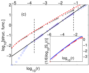
Figure 43: Log-log plots of $S_{3}^{\rm abs}(r)$ (dashed line), $S_{3}(r)$ (crosses), and $\langle(\delta^{+}v)^{3}\rangle$ (squares) versus $r$. The continuous line is a least-square fit to the range of points limited by two vertical dashed lines in the plot. Inset: An explicit check of the von Kármán–Howarth relation (7.27) from the simulations with $N=2^{20}$ reported in [91]. The dashed curve is the integral of the spatial part of the forcing correlation and the circles represent the numerical computation of the left-hand side.

As found in [91], the observed deviations of the scaling exponents from bifractality are actually due to the contamination by subleading terms in $S^{\rm abs}_{p}(r)$. To quantify this effect, let us focus on the third-order structure function ($p=3$) for which one measures $\zeta_{3}\approx 0.85\pm 0.02$ over nearly four decades (see figure 43). To estimate subleading terms we first notice that the third-order structure function $S_{3}(r)\equiv\langle(v(x+r)-v(x))^{3}\rangle$, which is defined, this time, without the absolute value, obeys an analog of the von Kármán–Howarth relation in fluid turbulence, namely

$$\frac{1}{6}S_{3}(r)=\int_{0}^{r}b(r^{\prime})\mathrm{d}r^{\prime},$$ (7.27)

where $b(\cdot)$ denotes the spatial part of the force correlation function, i.e. $\langle f(x+r,t^{\prime})f(x,t)\rangle=b(r)\delta(t-t^{\prime})$. This relation, together with the correlation (7.26) and $\beta=-1$, implies the behavior $S_{3}(r)\sim r\ln r$ at small separations $r$. As seen in figure 43, the graph of $S_{3}(r)$ in log-log coordinates indeed displays a significant curvature which is a signature of logarithmic corrections. The next step consists in decomposing the velocity increments $\delta_{r}v=v(x+r,t)-v(x,t)$ into their positive $\delta_{r}^{+}v$ and negative $\delta_{r}^{-}v$ parts. It is clear that

$$S^{\rm abs}_{3}(r)=-\left\langle(\delta_{r}^{-}v)^{3}\right\rangle+\left\langle(\delta_{r}^{+}v)^{3}\right\rangle,$$

$$S_{3}(r)=\left\langle(\delta_{r}^{-}v)^{3}\right\rangle+\left\langle(\delta_{r}^{+}v)^{3}\right\rangle,$$ (7.28)

so that $\left\langle(\delta_{r}^{+}v)^{3}\right\rangle=(S^{\rm abs}_{3}(r)+S_{3}(r))/2$. As seen in figure 43 the log-log plot of $\left\langle(\delta_{r}^{+}v)^{3}\right\rangle$ as a function of $r$ is nearly a straight line with slope $\approx 1.07$ very close to unity. This observation is confirmed in [91] by independently measuring the PDFs of positive and negative velocity increments. Assuming that $\left\langle(\delta_{r}^{+}v)^{3}\right\rangle\sim B\,r$, one obtains the following prediction for the small-$r$ behaviors of the third-order structure functions

$$S^{\rm abs}_{3}(r)\sim-Ar\ln r+B\,r,$$

$$S_{3}(r)\sim Ar\ln r+B\,r.$$ (7.29)

This suggests that the only difference in the small-separation behaviors of $S^{\rm abs}_{3}(r)$ and $S_{3}(r)$ is the sign in the balance between the leading term $\propto r\ln r$ and the subleading term $\propto r$. In a log-log plot this difference amounts to shifting the graph away from where it is most curved and thus makes it straighter, albeit with a (local) slope which is not unity. This explains why significant deviations from $1$ are observed for $\zeta_{3}$. Note that a similar approach can be used for higher-order structure functions. It leads for instance to $S_{4}(r)\approx Cr-Dr^{4/3}$, where $C$ and $D$ are two positive constants. The negative sign before the sub-leading term $(r^{4/3})$ is crucial. It implies that, for any finite $r$, a naive power-law fit to $S_{4}$ can yield a scaling exponent less than unity. The presence of sub-leading, power-law terms with opposite signs also explains the small apparent “anomalous” scaling behavior observed for other values of $p$ in the simulations. Note that similar artifacts involving two competing power-laws have been described in [16, 7].

The work reported in this section indicates that a naive interpretation of numerical measurements might result in predicting artificial anomalous scaling laws. In the case of Burgers turbulence for which high-resolution numerics are available and statistical convergence of the averages can be guaranteed, we have seen that it is not too difficult to identify the numerical artifacts which are responsible for such a masquerading. However this is not always the case. For instance, it seems reasonable enough to claim that attacking the problem of multiscaling in spatially extended nonlinear systems, such as Navier–Stokes turbulence, requires considerable theoretical insight that must supplement sophisticated and heavy numerical simulations and experiments. Note finally that, up to now, the question of the presence or not of anomalous scaling laws in the Burgers equation with a self-similar forcing with exponent $-1<\beta<0$ remains largely open.

8 Concluding remarks and open questions

This review summarizes recent work connected with the Burgers equation. Originally this model was introduced as a simplification of the Navier–Stokes equation with the hope of shedding some light on issues such as turbulence. This hope did not materialize. Nevertheless many of the interesting questions that have been addressed for Burgers turbulence are eventually transpositions of similar questions for Navier–Stokes turbulence. One particularly important instance is the issue of universality with respect to the form of the forcing and of the initial condition. For Burgers turbulence most of the universal features, such as scaling exponents or functional forms of PDF tails are dominated by the presence of shocks and other singularities in the solution. This applies both to the case of decaying turbulence driven by random initial conditions and randomly forced turbulence. In the latter case one is mostly interested in analysis of stationary properties of solutions, for example stationary distribution for velocity increments or gradients. Another set of questions is motivated by more mathematical considerations. It mainly concerns the construction of a stationary invariant measure when Burgers dynamics in a finite-size domain is supplemented by an external random source of energy. Again it has been shown that the presence of shocks, and in particular of global shocks, plays a crucial role in the construction of the statistically stationary solution. Both physical and mathematical questions lead to a similar answer: one first needs to describe and control shocks. The main message to retain for hydrodynamical turbulence is hence a strong confirmation of the common wisdom that it cannot be fully understood without a detailed description of singularities. Moreover, the behavior depends not only on the local structure of singularities, but also on their distribution at larger scales. Here a word of caution: for incompressible fully developped Navier–Stokes turbulence, we have no evidence that the universal scaling properties observed in experiments and simulations stem from real singularities. Indeed the issue of a finite-time blow-up of the three-dimensional Euler equation is still open (see, e.g. [56]). Another important observation that can be drawn from the study of Burgers turbulence is that both the tools used and the answers obtained strongly depend on the kind of setting one considers: decay versus forced turbulence, finite-size versus infinite-size systems, smooth versus self-similar forcing, etc.

Besides turbulence, the random Burgers equation has various applications in cosmology, in non-equilibrium statistical physics and in disordered media. Among them, the connection to the problem of directed polymers has attracted much attention. As already noted in the Introduction, there is a mathematical equivalence between the zero-viscosity limit of the forced Burgers equation and the zero-temperature limit for directed polymers. We have seen in section 5.4 that the so-called KPZ scaling, which usually is derived for a finite temperature, can be established can be established also in the zero-temperatur limit, using the action minimizer representation. Such an observation leads to two related questions: to what extent can the limit of zero temperature give an insight into finite-temperature polymer dynamics and how can the global minimizer formalism be extended to tackle the finite-temperature setting? It looks plausible that in polymer dynamics, or more generally in the study of random walks in a random potential, the trajectories carrying most of the Gibbs probability weight are defining corridors in space time. These objects can concentrate near the trajectories of global minimizers but, at the moment, there is no formalism to describe them, nor attempts to quantify their contribution to the Gibbs statistics.

Another important open question concerns the multi-dimensional extensions of the Burgers equation. As we have seen, when the forcing is potential, the potential character of the velocity field is conserved by the dynamics. This leads to the construction of stationary solutions which carry many similarities with the one-dimensional case. Up to now there is only limited understanding of what happens when the potentiality assumption of the flow is dropped. This problem has of course concrete applications in gas dynamics and for disperse inelastic granular media (see, e.g., [12]). An interesting question concerns the construction of the limit of vanishing viscosity, given that the Hopf–Cole transformation is inapplicable in the non-potential case. Understanding extensions of the viscous limiting procedure to the non-potential case might give new insight into the problem of the large Reynolds number limit in incompressible turbulence. Another question related to non-potential flow concerns the interactions between vorticity and shocks. For instance, in two dimensions the vorticity is transported by the flow. This results in its growth in the highly compressible regions of the flow. The various singularities of the velocity field should hence be strongly affected by the flow rotation and, in particular, the shocks are expected to have a spiraling structure.

We finish with few remarks on open mathematical problems. As we have seen in the one-dimensional case, one can rigorously prove hyperbolicity of the global minimizer. In the multi-dimensional case it is also possible to establish the existence and, in many cases, uniqueness of the global minimizer. However, the very important question of its hyperbolicity is still an open problem. If proven, hyperbolicity would allow for rigorous analysis of the regularity properties of the stationary solutions and of the topological shocks. There are many interesting problems – even basic issues of existence and uniqueness – in the non-compact case where at present a mathematical theory is basically absent. Finally, a very challenging open problem concerns the extension of the results on the evolution of matter inside shocks to the case of general Hamilton-Jacobi equations.

Over the years of our work on Burgers turbulence, we profited a lot from numerous discussions with Uriel Frisch whose influence on our work is warmly acknowledged. We also want to express our sincere gratitude to all of our collaborators: W. E, U. Frisch, D. Gomes, V.H. Hoang, R. Iturriaga, D. Khmelev, A. Mazel, D. Mitra, P. Padilla, R. Pandit, Ya. Sinai, A. Sobolevskiĭ, and B. Villone.
While writing this article, we benefited from discussions with M. Blank, I. Bogaevsky, K. Domelevo, V. Epstein, and A. Sobolevskiĭ. Finally, our thanks go to Itamar Procaccia whose encouragements and patience are greatly appreciated.

References

- [1] S. Anisov. Lowerbounds for the complexity of some 3-dimensional manifolds. preprint, 2001.
- [2] V. Arnol’d. Small denominators and problems of stability of motion in classical and celestial mechanics. Uspekhi Mat. Nauk, 18:91–192, 1963.
- [3] S. Aubry. The twist map, the extended Frenkel–Kontorova model and the devil’s staircase. Physica D, 7:240–258, 1983.
- [4] E. Aurell, U. Frisch, A. Noullez, and M. Blank. Bifractality of the Devil’s staircase appearing in Burgers equation with Brownian initial velocity. J. Stat. Phys., 88:1151–1164, 1997.
- [5] A.-L. Barabási and H.E. Stanley. Fractal Concepts in Surface Growth. Cambridge University Press, 1995.
- [6] J. Bec. Universality of velocity gradients in forced Burgers turbulence. Phys. Rev. Lett., 87:104501 (1–4), 2001.
- [7] J. Bec, M. Cencini, and R. Hillebrand. Heavy particles in incompressible flows: the large Stokes number asymptotics. Physica D, 226:11–22, 2007.
- [8] J. Bec and U. Frisch. Pdf’s of derivatives and increments for decaying Burgers turbulence. Phys. Rev. E, 61:1395–1402, 2000.
- [9] J. Bec, U. Frisch, and K. Khanin. Kicked Burgers turbulence. J. Fluid Mech., 416:239–267, 2000.
- [10] J. Bec, R. Iturriaga, and K. Khanin. Topological shocks in Burgers turbulence. Phys. Rev. Lett., 89:024501 (1–4), 2002.
- [11] J. Bec and K. Khanin. Forced Burgers equation in an unbounded domain. J. Stat. Phys., 113:741–759, 2003.
- [12] E. Ben-Naim, S. Y. Chen, G. D. Doolen, and S. Redner. Shocklike dynamics of inelastic gases. Phys. Rev. Lett., 83:4069–4072, 1999.
- [13] J.-D. Benamou and Y. Brenier. A computational fluid dynamics solution to the Monge–Kantorovich mass transfer problem. Numerische Mathematik, 84:375–393, 2000.
- [14] D. Bernard, K. Gawȩdzki, and A. Kupiainen. Anomalous scaling in the N-point functions of a passive scalar. Phys. Rev. E, 54:2564–2572, 1996.
- [15] D.P. Bertsekas. A new algorithm for the assignment problem. Math. Programming, 21:152–171, 1981.
- [16] L. Biferale, M. Cencini, A. Lanotte, and M. Sbragaglia. Anomalous scaling and universality in hydrodynamic systems with power-law forcing. New J. Phys., 4:37, 2004.
- [17] I.A. Bogaevsky. Perestroikas of shocks and singularities of minimum functions. Physica D, 173:1–28, 2002.
- [18] I.A. Bogaevsky. Matter evolution in burgulence. preprint, 2004.
- [19] S. Boldyrev. Burgers turbulence, intermittency, and non-universality. Phys. Plasmas, 5:1681–1687, 1998.
- [20] S. Boldyrev, T. Linde, and A. Polyakov. Velocity and velocity-difference distributions in Burgers turbulence. Phys. Rev. Lett., 93:184503, 2004.
- [21] J.-P. Bouchaud and M. Mézard. Velocity fluctuations in forced Burgers turbulence. Phys. Rev. E, 54:5116–5121, 1996.
- [22] J.-P. Bouchaud, M. Mézard, and G. Parisi. Scaling and intermittency in Burgers turbulence. Phys. Rev. E, 52:3656–3674, 1995.
- [23] Y. Brenier. Un algorithme rapide pour le calcul de transformées de Legendre-Fenchel discrètes. C. R. Acad. Sci. Paris Sér. I Math., 308:587–589, 1989.
- [24] Y. Brenier. Polar factorization and monotone rearrangement of vector-valued functions. Comm. Pure Appl. Math., 44:375–417, 1991.
- [25] Y. Brenier, U. Frisch, M. Hénon, G. Loeper, S. Matarrese, R. Mohayaee, and A. Sobolevskiĭ. Reconstruction of the early Universe as a convex optimization problem. Mon. Not. Roy. Astron. Soc., 346:501–524, 2003.
- [26] J.M. Burgers. Mathematical examples illustrating relations occuring in the theory of turbulent fluid motion. Verhand. Kon. Neder. Akad. Wetenschappen, Afd. Natuurkunde, Eerste Sectie, 17:1–53, 1939.
- [27] J.M. Burgers. The Nonlinear Diffusion Equation. D. Reidel, Dordrecht, 1974.
- [28] M. Chaves, G. Eyink, U. Frisch, and M. Vergassola. Universal decay of scalar turbulence. Phys. Rev. Lett., 86:2305–2308, 2000.
- [29] A. Chekhlov and V. Yakhot. Kolmogorov turbulence in a random-force-driven Burgers equation. Phys. Rev. E, 51:R2739–R2742, 1995.
- [30] A. Chekhlov and V. Yakhot. Kolmogorov turbulence in a random-force-driven Burgers equation: anomalous scaling and probability density functions. Phys. Rev. E, 52:5681–5684, 1995.
- [31] M. Chertkov, G. Falkovich, I. Kolokolov, and V. Lebedev. Normal and anomalous scaling of the fourth-order correlation function of a randomly advected passive scalar. Phys. Rev. E, 52:4924–4941, 1995.
- [32] D. Chowdhury, L. Santen, and A. Schadschneider. Statistical physics of vehicular traffic and some related systems. Phys. Rep., 329:199–329, 2000.
- [33] J.D. Cole. On a quasi-linear parabolic equation occurring in aerodynamics. Quart. Appl. Math., 9:225–236, 1951.
- [34] P. Coles and F. Lucchin. Cosmology : the origin and evolution of cosmic structures. J. Wiley and sons, 1995.
- [35] R. Dautray and J.-L. Lions. Analyse mathématique et calcul numérique pour les sciences et les techniques. Tome 3. Masson, Paris, 1985.
- [36] W. E. Aubry–Mather theory and periodic solutions for the forced Burgers equation. Comm. Pure Appl. Math., 52:0811–0828, 1999.
- [37] W. E, K. Khanin, A. Mazel, and Ya. Sinai. Probability distribution functions for the random forced Burgers equation. Phys. Rev. Lett., 78:1904–1907, 1997.
- [38] W. E, K. Khanin, A. Mazel, and Ya. Sinai. Invariant measures for Burgers equation with stochastic forcing. Ann. Math., 151:877–960, 2000.
- [39] W. E and E. Vanden Eijnden. Asymptotic theory for the probability density functions in Burgers turbulence. Phys. Rev. Lett., 83:2572–2575, 1999.
- [40] W. E and E. Vanden Eijnden. On the statistical solution of the riemann equation and its implications for Burgers turbulence. Phys. Fluids, 11:2149–2153, 1999.
- [41] W. E and E. Vanden Eijnden. Another note on Burgers turbulence. Phys. Fluids, 12:149–154, 2000.
- [42] W. E and E. Vanden Eijnden. Statistical theory for the stochastic Burgers equation in the inviscid limit. Comm. Pure Appl. Math., 53:852–901, 2000.
- [43] L. Evans. The perturbed test function method for viscosity solutions of nonlinear PDE. Proc. Roy. Soc. Edinburgh Sect. A, 111:359–375, 1989.
- [44] G.L. Eyink and D.J. Thomson. Free decay of turbulence and breakdown of self-similarity. Phys. Fluids, 12:477–479, 2000.
- [45] G.L. Eyink and J. Xin. Self-similar decay in the Kraichnan model of a passive scalar. J. Stat. Phys., 100:679–741, 2000.
- [46] G. Falkovich, K. Gawȩdzki, and M. Vergassola. Particles and fields in fluid turbulence. Rev. Mod. Phys., 73:913–976, 2001.
- [47] A. Fathi. Théorème KAM faible et théorie de Mather sur les systèmes lagrangiens. C. R. Acad. Sci. Paris Sér. I Math., 324:1043–1046, 1997.
- [48] A. Fathi. Weak KAM theorem in Lagrangian dynamics. Cambridge University Press, Cambridge, 2003.
- [49] W. Feller. An introduction to probability theory and its applications, volume 2. J. Wiley and sons, 1995.
- [50] W. Fleming and H. Soner. Controlled Markov processes and viscosity solutions. Springer–Verlag, New York, 1993.
- [51] J.-D. Fournier and U. Frisch. L’équation de Burgers déterministe et statistique. J. Méc. Théor. Appl., 2:699–750, 1983.
- [52] J. Frenkel and T. Kontorova. On the theory of plastic deformation and twinning. Acad. Sci. U.S.S.R. J. Phys., 1:137–149, 1939.
- [53] U. Frisch. Turbulence : the Legacy of A.N. Kolmogorov. Cambridge University Press, 1995.
- [54] U. Frisch, J. Bec, and B. Villone. Universal law for the distribution of density in the Burgers/adhesion model. Physica D, 152–153:620–635, 2001.
- [55] U. Frisch, S. Matarrese, R. Mohayaee, and A. Sobolevskiĭ. A reconstruction of the initial conditions of the Universe by optimal mass transportation. Nature, 417:260–262, 2002.
- [56] U. Frisch, T. Matsumoto, and J. Bec. Singularities of Euler flow? Not out of the blue! J. Stat. Phys., 113:761–781, 2003.
- [57] K. Gawȩdzki and A. Kupiainen. Anomalous scaling of the passive scalar. Phys. Rev. Lett., 75:3834–3837, 1995.
- [58] D. Gomes, R. Iturriaga, K. Khanin, and P. Padilla. Viscosity limit of stationary distributions for the random forced Burgers equation. Moscow Math. Journal, 5:613–631, 2005.
- [59] T. Gotoh and R.H. Kraichnan. Steady-state Burgers turbulence with large-scale forcing. Phys. Fluids, 10:2859–2866, 1998.
- [60] V. Gurarie and A. Migdal. Instantons in the Burgers equation. Phys. Rev. E, 54:4908–4914, 1996.
- [61] S. Gurbatov, A. Malakhov, and A. Saichev. Nonlinear Random Waves and Turbulence in Nondispersive Media: Waves, Rays, Particles. Manchester University Press, 1991.
- [62] S. Gurbatov and A. Saichev. Probability distribution and spectra of potential hydrodynamic turbulence. Radiophys. Quant. Electr., 27(4):303–313, 1984.
- [63] S. Gurbatov, S. Simdyankin, E. Aurell, U. Frisch, and G. Toth. On the decay of Burgers turbulence. J. Fluid Mech., 344:339–374, 1997.
- [64] F. Hayot and C. Jayaprakash. Multifractality in the stochastic Burgers equation. Phys. Rev. E, 54:4681–4684, 1996.
- [65] F. Hayot and C. Jayaprakash. From scaling to multiscaling in the stochastic Burgers equation. Phys. Rev. E, 56:4259–4262, 1997.
- [66] V.H. Hoang and K. Khanin. Random Burgers equation and Lagrangian systems in non-compact domains. Nonlinearity, 16:819–842, 2003.
- [67] E. Hopf. The partial differential equation . Comm. Pure Appl. Math., 3:201–230, 1950.
- [68] R. Iturriaga and K. Khanin. Two results on invariant measures for random Lagrangian systems and random Burgers equation. In Proceedings of the Third European Congress of Mathematics, Barcelona July 2000. Birkhauser, 2001. Progress in Mathematics.
- [69] R. Iturriaga and K. Khanin. Burgers turbulence and random Lagrangian systems. Comm. Math. Phys., 232:377–428, 2003.
- [70] H.R. Jauslin, H.O. Kreiss, and J. Moser. On the forced Burgers equation with periodic boundary conditions. In Differential equations: La Pietra 1996 (Florence), pages 133–153. Amer. Math. Soc., Providence, RI, 1999.
- [71] A. Jenkins, C.S. Frenk, F.R. Pearce, P.A. Thomas, J.M. Colberg, S.D. White, H.M. Couchman, J.A. Peacock, G. Efstathiou, and A.H. Nelson. Evolution of structure in cold dark matter Universes. Astrophys. J., 499:20–40, 1998.
- [72] J.V. José and E.J. Saletan. Classical dynamics: a contemporary approach. Cambridge University Press, 1998.
- [73] L.V. Kantorovich. On the translocation of masses. C. R. (Doklady) Acad. Sci. USSR, 37:199–201, 1942.
- [74] M. Kardar, G. Parisi, and Y.-C. Zhang. Dynamical scaling of growing interfaces. Phys. Rev. Lett., 56:889–892, 1986.
- [75] M. Kardar and Y.-C. Zhang. Scaling of directed polymers in random media. Phys. Rev. Lett., 58:2087–2090, 1987.
- [76] K. Khanin, D. Khmelev, and A. Sobolevskiĭ. A blow-up phenomenon in the Hamilton–Jacobi equation in an unbounded domain. In Proceedings of “Idempotent Mathematics and Mathematical Physics” workshop at the Erwin Schrödinger Institute in Vienna, 2003.
- [77] S. Kida. Asymptotic properties of Burgers turbulence. J. Fluid Mech, 93:337–377, 1979.
- [78] L. Kofman, D. Pogosyan, S. Shandarin, and A.L. Melott. Coherent structures in the universe and the adhesion model. Astrophys. J., 393:437–449, 1992.
- [79] A.N. Kolmogorov. On degeneration (decay) of isotropic turbulence in an incompressible viscous liquid. Dokl. Akad. Nauk SSSR, 31:538–540, 1941.
- [80] A.N. Kolmogorov. Théorie générale des systèmes dynamiques et mécanique classique. In Proceedings of the International Congress of Mathematicians, Amsterdam, 1954, Vol. 1, pages 315–333. Erven P. Noordhoff N.V., Groningen, 1957.
- [81] I. Kolokolov and V. Lebedev. About probability tails in forced Burgers turbulence. preprint, 2000.
- [82] S.N. Kružkov. Generalized solutions to Hamilton–Jacobi equations of the eikonal type. Mat. Sb. (N.S.), 98:450–493, 1975.
- [83] P.D. Lax. Hyperbolic systems of conservation laws II. Comm. Pure Appl. Math., 10:537–566, 1957.
- [84] M. Lesieur. Turbulence in Fluids. Fluid Mechanics and Its Applications 40. Kluwer, 1997.
- [85] P.-L. Lions. Generalized solutions of Hamilton-Jacobi equations, volume 69. Pitman Research Notes in Math., 1982.
- [86] J.N. Mather. Existence of quasi-periodic orbits for twist homeomorphisma of the annulus. Topology, 21:457–467, 1982.
- [87] S. Matveev. Complexity theory of three-dimensional manifolds. Acta Appl. Math., 19(2):101–130, 1990.
- [88] E. Medina, T. Hwa, M. Kardar, and Y.C. Zhang. Burgers equation with correlated noise: renormalization-group analysis and applications to directed polymers and interface growth. Phys. Rev. A, 39:3053–3075, 1989.
- [89] M. Mézard and G. Parisi. Interfaces in a random medium and replica symmetry breaking. J. Phys. A, 23:L1229–L1234, 1990.
- [90] M. Mézard, G. Parisi, and M.A. Virasoro. Spin glass theory and beyond. World Scientific, Singapore, 1987.
- [91] D. Mitra, J. Bec, R. Pandit, and U. Frisch. Is multiscaling an artifact in the stochastically forced Burgers equation. Phys. Rev. Lett., 84:194501, 2005.
- [92] S.A. Molchanov, D. Surgailis, and W.A. Woyczynski. Hyperbolic asymptotics in Burgers’ turbulence and extremal processes. Comm. Math. Phys., 168:209–226, 1995.
- [93] J. Moser. On invariant curves of area-preserving mappings of an annulus. Nachr. Akad. Wiss. Göttingen Math.-Phys. K1.II 1, pages 1–20, 1962.
- [94] A. Noullez and M. Vergassola. A fast Legendre transform algorithm and applications to the adhesion model. J. Sci. Comput., 9:259–281, 1994.
- [95] O.A. Oleinik. Discontinuous solutions of non-linear differential equations. Uspekhi Mat. Nauk (N.S.), 12(3):3–73, 1957.
- [96] S.A. Orszag. Statistical theory of turbulence. In R. Balian and J.L. Peube, editors, Fluid Dynamics, Les Houches 1973, pages 237–374. Gordon and Breach, 1977.
- [97] S. Ossia and M. Lesieur. Energy backscatter in LES of 3d incompressible isotropic turbulence. J. Turbulence, 1:007, 2000.
- [98] P.J.E. Peebles. Principles of Physical Cosmology. Princeton University Press, 1993.
- [99] A. Polyakov. Turbulence without pressure. Phys. Rev. E, 52:6183–6188, 1995.
- [100] I. Proudman and W.H. Reid. On the decay of a normally distributed and homogeneous turbulent velocity field. Phil. Trans. R. Soc. Lond. A, 247:163–189, 1954.
- [101] N. Provatas, T. Ala-Nissila, M. Grant, K. Elder, and L. Piche. Flame propagation in random media. Phys. Rev. E, 51:4232–4236, 1995.
- [102] H.A. Rose and P.-L. Sulem. Fully developed turbulence and statistical mechanics. J. Phys. France, 39:441–484, 1978.
- [103] B. Schraiman and E. Siggia. Anomalous scaling of a passive scalar in turbulent flow. C.R. Acad. Sci., 321:279–284, 1995.
- [104] Z.S. She, E. Aurell, and U. Frisch. The inviscid Burgers equation with initial data of Brownian type. Commun. Math. Phys., 148:623–641, 1992.
- [105] Ya. Sinai. Statistics of shocks in solutions of inviscid Burgers equation. Commun. Math. Phys., 148:601–622, 1992.
- [106] A. Sobolevskiĭ. Periodic solutions of the Hamilton–Jacobi equation with a periodic non-homogeneous term and Aubry–Mather theory. Mat. Sbornik, 190:1487–1504, 1999.
- [107] M. Vergassola, B. Dubrulle, U. Frisch, and A. Noullez. Burgers’ equation, Devil’s staircases and the mass distribution for large-scale structures. Astron. Astrophys., 289:325–356, 1994.
- [108] A.I. Vol’pert. Spaces BV and quasilinear equations. Mat. Sb., 73:255–302, 1967.
- [109] T. von Kármán and L. Howarth. On the statistical theory of isotropic turbulence. Proc. R. Soc. Lond. A, 164:192–215, 1938.
- [110] W. Woyczyński. Burgers-KPZ Turbulence: Gottingen lectures. Springer–Verlag, New York, 1998.
- [111] V. Yakhot and A. Chekhlov. Algebraic tails of probability density functions in the random-force-driven Burgers turbulence. Phys. Rev. Lett., 77:3118–3121, 1996.
- [112] Ya. Zel’dovich. Gravitational instability: an approximate theory for large density perturbations. Astron. Astrophys., 5:84–89, 1970.