Asteroseismic Signatures of Stellar Magnetic Activity Cycles

Abstract

Observations of stellar activity cycles provide an opportunity to study magnetic dynamos under many different physical conditions. Space-based asteroseismology missions will soon yield useful constraints on the interior conditions that nurture such magnetic cycles, and will be sensitive enough to detect shifts in the oscillation frequencies due to the magnetic variations. We derive a method for predicting these shifts from changes in the Mg ii activity index by scaling from solar data. We demonstrate this technique on the solar-type subgiant $\beta$ Hyi, using archival International Ultraviolet Explorer spectra and two epochs of ground-based asteroseismic observations. We find qualitative evidence of the expected frequency shifts and predict the optimal timing for future asteroseismic observations of this star.

1 Introduction

Astronomers have been making telescopic observations of sunspots since the time of Galileo, gradually building an historical record showing a periodic rise and fall in the number of sunspots every $\sim$11 years. We now know that sunspots are regions with an enhanced local magnetic field, so this 11-year cycle actually traces a variation in surface magnetism. Attempts to understand this behavior theoretically often invoke a combination of differential rotation, convection, and meridional flow to modulate the field through a magnetic dynamo (e.g., see Rempel, 2006; Dikpati & Gilman, 2006).

Although we can rarely observe spots on other solar-type stars directly, these areas of concentrated magnetic field produce strong emission in the Ca ii H and K resonance lines in the optical, and the Mg ii h and k lines in the ultraviolet. Wilson (1978) was the first to demonstrate that many solar-type stars exhibit long-term cyclic variations in their Ca ii H and K emission, analogous to those seen in full-disc solar observations through the magnetic activity cycle. Early analysis of these data revealed an empirical correlation between the mean level of magnetic activity and the rotation period normalized by the convective timescale (Noyes et al., 1984a), as well as a relation between the rotation rate and the period of the observed activity cycle (Noyes et al., 1984b), which generally supports a dynamo interpretation.

Significant progress in dynamo modeling unfolded after helioseismology provided detailed constraints on the Sun’s interior structure and dynamics. These observations also established that variations in the mean strength of the solar magnetic field lead to significant shifts ($\sim$0.5 $\mu$Hz) in the frequencies of even the lowest-degree p-modes (Libbrecht & Woodard, 1990; Salabert et al., 2004). These shifts can provide independent constraints on the physical mechanisms that drive the solar dynamo, through their influence on the outer boundary condition for the pulsation modes. They are thought to arise either from changes in the near-surface propagation speed due to a direct magnetic perturbation (Goldreich et al., 1991), or from a slight decrease in the radial component of the turbulent velocity in the outer layers and the associated changes in temperature (Dziembowski & Goode, 2004, 2005).

Space-based asteroseismology missions, such as MOST (Walker et al., 2003), CoRoT (Baglin et al., 2006), and Kepler (Christensen-Dalsgaard et al., 2007) will soon allow additional tests of dynamo models using other solar-type stars (see Chaplin et al., 2007). High precision time-series photometry from MOST has already revealed latitudinal differential rotation in two solar-type stars (Croll et al., 2006; Walker et al., 2007), and the long-term monitoring from future missions is expected to produce asteroseismic measurements of stellar convection zone depths (Monteiro et al., 2000; Verner et al., 2006). By combining such observations with the stellar magnetic activity cycles documented from long-term surveys of the Ca ii or Mg ii lines, we can extend the calibration of dynamo models from the solar case to dozens of independent sets of physical conditions.

The G2 subgiant $\beta$ Hyi is the only solar-type star that presently has both a known magnetic activity cycle (Dravins et al., 1993) and multiple epochs of asteroseismic observations (Bedding et al., 2001, 2007). In this paper we reanalyze archival International Ultraviolet Explorer (IUE) spectra for an improved characterization of the magnetic cycle in this star, and we use it to predict the activity related shifts in the observed radial p-mode oscillations. We compare these predictions with recently published asteroseismic data, and we suggest the optimal timing of future observations to maximize the amplitude of the expected p-mode frequency shifts.

2 Archival IUE spectra

The activity cycle of $\beta$ Hyi was studied by Dravins et al. (1993), who used high resolution IUE data of the Mg ii resonance lines over 11 years, from June 1978 to the end of October 1989. They considered these data to be consistent with a cycle period between 15 and 18 years. Since the work of Dravins et al., a significant number of additional IUE spectra were obtained by E. Guinan from early 1992 to the end of 1995. Our analysis of all of these spectra reveals the beginning of a new cycle in 1993-1994.

In 1997, the IUE project reprocessed the entire database using improved and uniform reduction procedures (“NEWSIPS”). Using the NEWSIPS merged high resolution extracted spectra, we have reanalyzed the entire IUE dataset containing useful echelle data of the Mg ii lines. Data were excluded when the NEWSIPS software mis-registered the spectral orders, when continuum data near 279.67 nm were saturated, or when continuum data were more than $1\sigma$ below the mean (to reject additional poorly registered spectral orders) or more than $1.5\sigma$ above the mean.

The classic definition of the Mg ii index (Heath & Schlesinger, 1986) uses wing irradiances at 276 and 283 nm. The wings in their formulation had to be so far away from the cores due to the 1.1 nm spectral bandpass of their instrument. In the IUE spectra, pixels at those wavelengths are saturated, so the photospheric reference levels need to be measured much closer to the emission cores. Snow & McClintock (2005) have shown that at moderate resolution the variability of the inner wings of the Mg ii absorption feature is very similar to the variability of the classic wing irradiances. Therefore, we can construct a modified Mg ii index using only the unsaturated IUE data that still captures the full chromospheric variability.

The chromospheric line cores (0.14 and 0.12 nm wide bandpasses centered at 279.65 and 280.365 nm, in vacuo) and two bands in the photospheric wings of the lines (0.4 nm wide bands, edge-smoothed with cosine functions, centered at 279.20 and 280.70 nm) were integrated, and the ratio of total core to total wing fluxes was determined. Figure 1 shows the core to wing indices determined from each usable spectrum from 1978 to the end of 1995. The post-1992 data permit us to revise the cycle period estimate downwards to $\sim$12.0 years, with more confidence than was previously possible. This period was derived by fitting a simple sinusoid to the data using the genetic algorithm PIKAIA (Charbonneau, 1995). The optimal fit yields minima at 1980.9 and 1992.8, and a maximum at 1986.9. The fit suggests that the next maximum occurred in 1998.8, a minimum in 2004.8, and a future maximum predicted for 2010.8. The reduced $\chi^{2}$ of the fit was calculated using flux uncertainties for individual IUE observations of 7%, estimated from the variation in the ratios of the two wing fluxes, which vary far less than this in the SOLSTICE solar data. This reduced $\chi^{2}$ has a minimum value of 0.77. The probability of such a value occurring at random is 24%, whereas a $\chi^{2}$ of $1.1$ has a random probability of 76%. The $\chi^{2}=1.1$ hypersurface contours suggests that the uncertainties are roughly $\pm 1$ yr for the phase and ${}^{+3.0}_{-1.7}$ yr for the period, making our new period estimate marginally consistent with the range quoted by Dravins et al. (1993). The $\chi^{2}$ contours are ovals because these uncertainties are correlated, allowing us to set the following formal limits on the epochs of maximum: 1986.1–1988.0, 1997.5–2002.4, and 2007.8–2017.8. These large uncertainties reinforce the need for an activity cycle monitoring program specifically for the southern hemisphere.

Figure 1: Core to wing ratios of the summed Mg ii h and k lines determined from IUE high dispersion observations of $\beta$ Hyi (small points) and 3-month seasonal averages with the uncertainties used in the evaluation of $\chi^{2}$ shown as error bars (large points). The curve is an optimized simple sinusoid fit obtained using a genetic algorithm applied to the seasonally averaged data, intended only to estimate the period and phase of the stellar activity cycle, which is listed in the legend. The IUE index is shown on the left, while the corresponding NOAA index is shown on the right.

To compare the IUE Mg ii index measurements to the National Oceanic & Atmospheric Administration (NOAA) composite data of solar activity, we must determine the appropriate scaling factor. The SOLar-STellar Irradiance Comparison Experiment (SOLSTICE) on the SOlar Radiation and Climate Experiment (SORCE; McClintock et al., 2005) measures the solar irradiance every day, and has a resolution of 0.1 nm in this region. We convolved the IUE spectra with the SOLSTICE instrument function and then measured the wings and cores of both solar and stellar data in exactly the same way. In particular, we used 279.15-279.35 nm as the blue wing, and 280.65-280.85 nm for the red wing. The emission cores were defined as 279.47-279.65 nm and 280.21-280.35 nm. We determined the relation between the SOLSTICE modified Mg ii index and the NOAA long-term record using a standard linear regression method (see Snow et al., 2005; Viereck et al., 2004). Since the modified IUE data has the same bandpass as the SOLSTICE data, the scaling factors derived from SOLSTICE solar data will also apply to the stellar IUE data. The Mg ii index for $\beta$ Hyi scaled to the NOAA composite data is shown on the right axis of Figure 1. For the analysis in Section 3, we adopt a full amplitude of $\Delta i_{\rm MgII}=0.015$ in the NOAA index.

3 Scaling p-mode shifts from solar data

In general, we can evaluate activity related frequency shifts from the variational expression,

$$\Delta\nu_{j}={\int d^{3}\mbox{\boldmath{$x$}}{\cal K}_{j}{\cal S}\over 2I_{j}\nu_{j}},$$ (1)

where

$$I_{j}=\int d^{3}\mbox{\boldmath{$x$}}\rho|\mbox{\boldmath{$\xi$}}|^{3}\equiv R^{5}\bar{\rho}\tilde{I}$$ (2)

is the mode inertia, $j\equiv(n,\ell,m)$, and we need to know both the source ${\cal S}(\mbox{\boldmath{$x$}})$ and the corresponding kernels ${\cal K}(\mbox{\boldmath{$x$}})$. The source must include the direct influence of the growing mean magnetic field, as well as its indirect effect on the convective velocities and temperature distribution. Separate kernels for these effects were calculated by Dziembowski & Goode (2004), but there is no theory available to calculate the combined source. Moreover, it is unclear whether the model of small-scale magnetic fields, adopted from Goldreich et al. (1991), is adequate. Therefore, we will attempt to formulate an extrapolation of the solar p-mode frequency shifts based on changes in the Mg ii activity index measured for the Sun and for $\beta$ Hyi in Section 2.

For p-modes, the dominant terms in all of the kernels are proportional to $|\mbox{\rm div}\mbox{\boldmath{$\xi$}}|^{2}$. Thus, we write

$${\cal K}_{j}(\mbox{\boldmath{$x$}})=|\mbox{\rm div}\mbox{\boldmath{$\xi$}}_{j}|^{2}=q_{j}(D)Y_{\ell}^{m},$$ (3)

where $D$ is the depth beneath the photosphere. A model-dependent coefficient will be absorbed into the source, which we write in the form

$${\cal S}(\mbox{\boldmath{$x$}})=\sum_{k=0}{\cal S}_{k}(D)P_{2k}(\cos\theta).$$ (4)

Solar data imply that ${\cal S}$ is strongly concentrated near the photosphere. Therefore data from all p-modes, regardless of their $\ell$ value, may be used to constrain ${\cal S}$. We might also expect that the source normalization is correlated with the Mg ii index.

If we want to calculate $\Delta\nu_{j}$ according to Eq. (1), we need all terms of ${\cal S}$ up to $k=\ell$. To assess the solar ${\cal S}$, we have measurements of the centroid shifts and the even-$a$ coefficients (see Dziembowski & Goode, 2004). For the $\ell=0$ modes we only need to know the $k=0$ term, and for this the centroid data are sufficient. Let us begin with this simple case.

3.1 Radial modes

Theoretical arguments and the observed pattern of solar frequency changes suggest that the dominant source must be localized near the photosphere. Therefore, it seems reasonable to try to fit the measured p-mode frequency shifts by adopting

$${\cal S}_{0}(D)=1.5\times 10^{-11}A_{0}\delta(D-D_{c})~{}\mu{\rm Hz}^{2},$$ (5)

with adjustable parameters $A_{0}$ and $D_{c}$. The numerical coefficient is arbitrary, and was chosen for future convenience. With Eqs. (3-5), we get from Eq. (1)

$$\Delta\nu_{j}=A_{0}{R\over M}Q_{j}(D_{c}),$$ (6)

where $R$ and $M$ (as well as $L$ below) are expressed in solar units, frequencies are expressed in $\mu$Hz, and

$$Q_{j}=1.5\times 10^{-11}{q_{j}\over\nu_{j}\tilde{I}_{j}}.$$ (7)

The solar values of $A_{0}$ and $D_{c}$ can be determined by fitting the centroid frequency shifts $\Delta\nu_{j}$ from SOHO MDI data for p-modes with various spherical degrees, $\ell$. Since at $n=1$ the approximation inherent in Eq. (3) is questionable, we use data only for the higher orders.

For the Sun, we have

$$A_{0,\odot}(D_{c})=\overline{\left(w_{j}\Delta\nu_{j}\over Q_{j}\right)},$$ (8)

where $\Delta\nu_{j}$ are the measured shifts and $w_{j}$ are the relative weights. The values of $Q_{j}$ are calculated from a solar model. The best value of $D_{c}$ is that which minimizes the dispersion,

$$\sigma(D_{c})=\sqrt{\overline{\left[w_{j}\left(A_{0,\odot}-{\Delta\nu_{j}\over Q_{j}}\right)^{2}\right]}}.$$ (9)

It is also reasonable to assume that $A_{0}$ should be proportional to the change in the Mg ii activity index, $\Delta i_{\rm MgII}$, and that $D_{c}$ is proportional to the pressure scale height at the photosphere. Thus, we have

$$A_{0}=A_{0,\odot}{\Delta i_{\rm MgII}\over\Delta i_{{\rm MgII},\odot}}$$ (10)

and

$$D_{c}\propto H_{p}=D_{c,\odot}L^{0.25}{R^{1.5}\over M}.$$ (11)

Figure 2: Determinations of $A_{0,\odot}$ from SOHO MDI data with $D_{c}$ fixed at 0.3 Mm (top panel), and using the optimal value of $D_{c}$ for each set (middle panel), with the corresponding changes in the Mg ii index from the NOAA composite data (bottom panel).

To determine $A_{0,\odot}$, we used SOHO MDI frequencies for all p_n modes with $n>1$, $\ell$ from 0 to $\sim$181, and $\nu$ between 2.5 and 4.2 mHz. The data were combined into 38 sets, typically covering 0.2 years. We averaged the frequencies from the first 5 sets, corresponding to solar minimum (1996.3-1997.3), and subtracted them from the frequencies in subsequent sets to evaluate $A_{0,\odot}$ using Eq. (8). The results are shown in Figure 2, where the points in the top panel were obtained at fixed $D_{c}=0.3$ Mm, which is representative of the highest activity period. In the middle panel, the value of $D_{c}$ was determined separately for each set and the error bars represent the dispersion. In the bottom panel, we show the corresponding changes in the solar Mg ii index calculated from NOAA composite data. A tight correlation between $A_{0,\odot}$ and $\Delta i_{{\rm MgII},\odot}$ is clearly visible.

Although the optimum value of $D_{c}$ is weakly correlated with the activity level, the dispersion changes very little between $D_{c}=0.2$ and 0.4 Mm, so we fixed the value of $D_{c,\odot}$ to 0.3 Mm. In Figure 3, we show the quality of the fit to the observed frequency shifts for selected p-modes using Eq. (6) with the adopted value of $D_{c}$. The upper panel shows the frequency shifts averaged from four sets of data near the activity maximum in 2002.0, while the lower panel shows $\Delta\nu_{j}/Q_{j}$. Note that most of the frequency and $\ell$-dependence appears to have been fit by our parametrization. The slight rise at frequencies below 3 mHz could be eliminated by allowing a spread of the kernel toward lower depths. However, since the signal is more significant at higher frequencies, we believe that adding a finite radial extent would be an unnecessary complication.

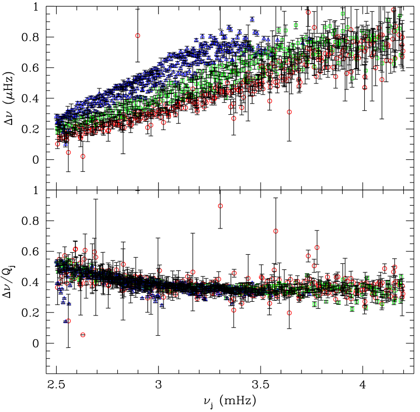
Figure 3: The observed p-mode frequency shifts averaged from four sets of data obtained near the solar maximum in 2002.0 (top panel), and the same shifts normalized by $Q_{j}$ (bottom panel) showing that most of the frequency and $\ell$-dependence is included in our parametrization. Different symbols show the roughly equal number of modes with $\ell\leq 30$ (circles), $31\leq\ell\leq 75$ (squares), and $76\leq\ell\leq 181$ (triangles).

There were two activity maxima during solar cycle 23. The first was centered near 2000.6 and the second at 2002.0. The average values of ($A_{0,\odot},\Delta i_{{\rm MgII},\odot}$) are (0.3116, 0.0135) for five data sets around the first maximum and (0.3669, 0.0178) for four data sets around the second maximum. For future applications, we adopt $A_{0,\odot}/\Delta i_{{\rm MgII},\odot}=22$.

With this specification, we get from Eqs. (6) and (10)

$$\Delta\nu_{j}=3.3\times 10^{-10}\Delta i_{\rm MgII}{R\over M}{q_{j}(D_{c})\over\nu_{j}\tilde{I}_{j}},$$ (12)

where

$$D_{c}=0.3L^{0.25}{R^{1.5}\over M}\mbox{ mM}$$ (13)

and again frequencies are expressed in $\mu$Hz, while $R$, $M$, and $L$ are in solar units. This is our expression for predicting the radial p-mode frequency shifts on the basis of changes in the NOAA composite Mg ii index. In Table 1, we list the frequency shifts ($\Delta\nu_{j}$) calculated from Eq. (12) for the radial modes of $\beta$ Hyi observed by Bedding et al. (2007), adopting $\Delta i_{\rm MgII}=0.015$. The mode parameters $q_{j}$ and $\tilde{I}_{j}$ were calculated from a model of $\beta$ Hyi generated using the Aarhus STellar Evolution Code (ASTEC; Christensen-Dalsgaard, 1982).

3.2 Non-radial modes

Now from Eqs. (1) and (4). we have

$$\Delta\nu_{nlm}={\sum_{k=0}^{\ell}{\cal S}_{k}\kappa_{k,lm}\over 2I_{nl}\nu_{nl}},$$ (14)

where,

$$\kappa_{k,lm}=\int d\theta d\phi|Y_{\ell}^{m}|^{2}P_{2k}(\cos\theta)\sin\theta.$$ (15)

As in Eq. (5), we can adopt

$${\cal S}_{k}(D)=1.5\times 10^{-11}A_{k}\delta(D-D_{c,k})~{}\mu{\rm Hz}^{2}.$$ (16)

For $k>0$, the solar amplitudes $A_{k}$ and effective depths, $D_{c,k}$ can be determined by fitting measurements of shifts in the $a_{2k}$ coefficients. The relation is

$$\Delta a_{2k,\ell m}=A_{k}Z_{k,\ell}Q_{k,n\ell}(D_{c,k}),$$ (17)

where

$$Z_{k,\ell}=(-1)^{k}{(2k-1)!!\over k!}{(2\ell+1)!!\over(2\ell+2k+1)!!}{(\ell-1)!\over(\ell-k)!}$$ (18)

(cf. Dziembowski & Goode, 2004, their Eq. 2), and

$$Q_{k,n\ell}=1.5\times 10^{-11}{q_{n\ell}(D_{c,k})\over\nu_{j}\tilde{I}_{n\ell}}$$ (19)

(compare to our Eq. 7).

The prediction of frequency shifts for non-radial modes requires an additional assumption of the same scaling for all required $A_{k}$ amplitudes, which amounts to assuming the same Butterfly diagram as observed on the Sun. Moreover, since the shifts depend on $|m|$ and multiplets are not expected to be resolved, we need to adopt the inclination angle ($i$) to correctly weight the contributions from all of the components. Since we do not know $i$ for $\beta$ Hyi, we restrict our numerical predictions to the radial modes.

Table 1: Predicted radial p-mode frequency shifts between activity maximum and minimum for $\beta$ Hyi, calculated with Eq. (12) and adopting $\Delta i_{\rm MgII}=0.015$. Frequencies are from Table 1 of Bedding et al. (2007).

$n$	Frequency ($\mu$Hz)	$\Delta\nu_{j}$ ($\mu$Hz)
13	833.72	0.061
14	889.87	0.091
15	945.64	0.116
16	1004.21	0.139
17	1062.06	0.168
18	1118.93	0.199
19	1176.48	0.234

4 Asteroseismic Observations

The detection of solar-like oscillations in $\beta$ Hyi was first reported by Bedding et al. (2001), and later confirmed by Carrier et al. (2001). These two detections of excess power were based on data obtained during a dual-site campaign organized in June 2000 using the 3.9-m Anglo-Australian Telescope (AAT) at Siding Spring Observatory and the 1.2-m Swiss telescope at the European Southern Observatory (ESO) in Chile. Both sets of observations measured a large frequency separation between 56-58 $\mu$Hz, but neither was sufficient for unambiguous identification of individual oscillation modes.

Nearly 30 individual modes in $\beta$ Hyi with $\ell$=0-2 were detected during a second dual-site campaign organized in September 2005, and reported by Bedding et al. (2007). The authors also reanalyzed the combined 2000 observations using an improved extraction algorithm for the AAT data, allowing them to identify some of the same oscillation modes at this earlier epoch. Motivated by the first tentative detection of a systematic frequency offset between two asteroseismic data sets for $\alpha$ Cen A (0.6$\pm$0.3 $\mu$Hz; Fletcher et al., 2006), they compared the two epochs of observation for $\beta$ Hyi and found the 2005 frequencies to be systematically lower than those in 2000 by 0.1$\pm$0.4 $\mu$Hz, consistent with zero but also with the mean value in Table 1.

A comparison of the individual modes from these two data sets (T. Bedding, private communication) allows a further test of our predictions. Of the 14 modes that were detected with S/N $>4$ in both 2000 and 2005, only one was known to be a radial ($\ell=0$) mode, while four had $\ell=1$, three had $\ell=2$, two were mixed modes, and four had no certain identification. Without a known inclination, we can only calculate the shifts for radial modes, but the magnitude of the shift is largest at high frequencies (see Table 1). Fortunately, the radial mode that is common to both data sets ($\ell=0$, $n=18$) has a frequency above the peak in the envelope of power, improving our chances of measuring a shift. The best estimate of the mode frequency from each data set comes from the noise-optimized power spectrum, since this maximizes the S/N of the observed peaks. The noise-optimized frequency for the $\ell=0$, $n=18$ mode was 1119.06 and $1118.89~{}\mu$Hz in the 2000 and 2005 data sets, respectively. Considering the quoted uncertainty for this mode from Table 1 of Bedding et al. (2007), the frequency was 0.17$\pm$0.62 $\mu$Hz lower in 2005 than in 2000, again consistent with zero but similar to the predicted shift for this mode in Table 1.

5 Discussion

Our reanalysis of archival IUE spectra for $\beta$ Hyi allows us to test our predictions of the relationship between the stellar activity cycle and the systematic frequency shift measured from multi-epoch asteroseismic observations. The optimal period and phase of the activity cycle from Section 2 suggest that $\beta$ Hyi was near magnetic minimum (2004.8) during the 2005 observations (2005.7), while it was descending from magnetic maximum (1998.8) during the 2000 campaign (2000.5). The systematic frequency shift of 0.1$\pm$0.4 $\mu$Hz reported by Bedding et al. (2007) between these two epochs, and the observed shift of 0.17$\pm$0.62 $\mu$Hz in the only radial mode ($\ell=0$, $n=18$) common to both data sets are not statistically significant. They are both nominally in the direction predicted by our analysis of the activity cycle (lower frequencies during magnetic minimum) and they have approximately the expected magnitude (cf. Table 1), but the formal uncertainties on the period and phase of the activity cycle do not permit a definitive test.

Future asteroseismic observations of $\beta$ Hyi would sample the largest possible frequency shift relative to the 2005 data if timed to coincide with the magnetic maximum predicted for $2010.8^{+7}_{-3}$. Long-term monitoring of the stellar activity cycles of this and other southern asteroseismic targets (e.g. $\alpha$ Cen A/B, $\mu$ Ara, $\nu$ Ind), which are not included in the Mt. Wilson sample, would allow further tests of our predictions. For asteroseismic targets that have known activity cycles from long-term Ca ii H and K measurements (e.g. $\epsilon$ Eri, Procyon), it would be straightforward to calibrate our predictions to this index from comparable solar observations.

While our current analysis involves a simple scaling from solar data, future observations may allow us to refine magnetic dynamo models by looking for deviations from this scaling relation and attempting to rectify the discrepancies. By requiring the models to reproduce the observed activity cycle periods and amplitudes—along with the resulting p-mode shifts and their frequency dependence for a variety of solar-type stars at various stages in their evolution—we can gradually provide a broader context for our understanding of the dynamo operating in our own Sun.

References

- Baglin et al. (2006) Baglin, A., et al. 2006, ESA SP-624: Proceedings of SOHO 18/GONG 2006/HELAS I, Beyond the spherical Sun, 18
- Bedding et al. (2001) Bedding, T. R., et al. 2001, ApJ, 549, L105
- Bedding et al. (2007) Bedding, T. R., et al. 2007, ApJ, in press (astro-ph/0703747)
- Carrier et al. (2001) Carrier, F., et al. 2001, A&A, 378, 142
- Chaplin et al. (2007) Chaplin, W. J., et al. 2007, MNRAS, in press
- Charbonneau (1995) Charbonneau, P. 1995, ApJS, 101, 309
- Christensen-Dalsgaard (1982) Christensen-Dalsgaard, J. 1982, MNRAS, 199, 735
- Christensen-Dalsgaard et al. (2007) Christensen-Dalsgaard, J., et al. 2007, Comm. in Astero., in press (astro-ph/0701323)
- Croll et al. (2006) Croll, B., et al. 2006, ApJ, 648, 607
- Dikpati & Gilman (2006) Dikpati, M., & Gilman, P. A. 2006, ApJ, 649, 498
- Dravins et al. (1993) Dravins, D., et al. 1993, ApJ, 403, 396
- Dziembowski & Goode (2004) Dziembowski, W. A., & Goode, P. R. 2004, ApJ, 600, 464
- Dziembowski & Goode (2005) Dziembowski, W. A., & Goode, P. R. 2005, ApJ, 625, 548
- Fletcher et al. (2006) Fletcher, S. T., et al. 2006, MNRAS, 371, 935
- Goldreich et al. (1991) Goldreich, P., et al. 1991, ApJ, 370, 752
- Heath & Schlesinger (1986) Heath, D. F., & Schlesinger, B. M. 1986, JGR, 91, 8672
- Libbrecht & Woodard (1990) Libbrecht, K. G., & Woodard, M. F. 1990, Nature, 345, 779
- McClintock et al. (2005) McClintock, W. E., et al. 2005, Sol. Phys., 230, 225
- Monteiro et al. (2000) Monteiro, M. J. P. F. G., et al. 2000, MNRAS, 316, 165
- Noyes et al. (1984a) Noyes, R. W., et al. 1984a, ApJ, 279, 763
- Noyes et al. (1984b) Noyes, R. W., et al. 1984b, ApJ, 287, 769
- Rempel (2006) Rempel, M. 2006, ApJ, 647, 662
- Salabert et al. (2004) Salabert, D., et al. 2004, A&A, 413, 1135
- Snow & McClintock (2005) Snow, M., & McClintock, W. E. 2005, Proc. SPIE, 5901, 337
- Snow et al. (2005) Snow, M., et al. 2005, Sol. Phys., 230, 325
- Verner et al. (2006) Verner, G. A., Chaplin, W. J., & Elsworth, Y. 2006, ApJ, 638, 440
- Viereck et al. (2004) Viereck, R. A., et al. 2004, Space Weather, 2, 5
- Walker et al. (2003) Walker, G., et al. 2003, PASP, 115, 1023
- Walker et al. (2007) Walker, G., et al. 2007, ApJ, in press
- Wilson (1978) Wilson, O. C. 1978, ApJ, 226, 379