Measuring energy dependent polarization in soft gamma-rays using Compton scattering in PoGOLite

Abstract

Linear polarization in X- and gamma-rays is an important diagnostic of many astrophysical sources, foremost giving information about their geometry, magnetic fields, and radiation mechanisms. However, very few X-ray polarization measurements have been made, and then only mono-energetic detections, whilst several objects are assumed to have energy dependent polarization signatures.

In this paper we investigate whether detection of energy dependent polarization from cosmic sources is possible using the Compton technique, in particular with the proposed PoGOLite balloon-experiment, in the 25–100 keV range. We use Geant4 simulations of a PoGOLite model and input photon spectra based on Cygnus X-1 and accreting magnetic pulsars (100 mCrab). Effective observing times of 6 and 35 hours were simulated, corresponding to a standard and a long duration flight respectively. Both smooth and sharp energy variations of the polarization are investigated and compared to constant polarization signals using chi-square statistics.

We can reject constant polarization, with energy, for the Cygnus X-1 spectrum (in the hard state), if the reflected component is assumed to be completely polarized, whereas the distinction cannot be made for weaker polarization. For the accreting pulsar, constant polarization can be rejected in the case of polarization in a narrow energy band with at least 50% polarization, and similarly for a negative step distribution from 30% to 0% polarization.

, , , , , , , , , , , , , , , , , , , , , , , , ,

1 Introduction

In the areas of spectral and temporal studies, X-ray and gamma-ray astronomers have been given a wealth of data on a wide range of objects. Polarization has long been predicted to play a crucial role in determining physical and geometrical parameters in many astrophysical sources, thereby discriminating among current models. However, there have so far been very few measurements of polarization at these energies. In light of this, the possibility to detect energy dependent polarization has hardly been discussed at all in the literature. In this paper, we present the results from simulations of a dedicated soft gamma-ray polarimeter using Compton scattering, and study the response when the degree of polarization varies with the energy of the emitted photons. While energy-dependent polarization is expected from many sources, its detection requires an instrument of sufficiently good energy response. The Compton polarimeter presented in this paper utilizes plastic scintillators, which are relatively inefficient for energy depositions below a few keV. Thus, simulations are necessary to determine how sensitive the instrument is and how large variations must be for detection.

We begin by describing the organisation of the paper. The remainder of this section is devoted to giving a background of polarimetry in the X/$\gamma$-ray regime, and an overview of the scientific motivation for such measurements. In Section 2 we focus on polarimetry using Compton scattering and describe an instrument design based on this technique. We then present the set-up of our simulation of the instrument in Section 3, and the results of the simulations in Section 4. Finally, in Sections 5 and 6, we discuss and summarise our results.

1.1 Measurement of polarization

The aim of any polarimetric measurement is to determine the degree and direction of polarization of incident radiation. When combined with the traditionally measured quantities of energy and time, polarimetry has the potential to double the parameter space available. As such, it can be a powerful tool to discriminate between physical models proposed for a given source.

Historically, polarimetry has proven very successful at optical and radio wavelengths. In these bands, it has been extensively used to probe both radiation physics and geometry of sources (see, e.g., [1]). In the X-ray regime, however, the results are more meagre. Early rocket observations measured X-ray polarization from the Crab Nebula [2]. This result was later confirmed by the Orbiting Solar Observatory 8 (OSO-8, measuring a polarization degree of $19.2\%\pm 1.0\%$, [3, 4]), the only satellite mission carrying a dedicated polarimeter to date. As the design was based on Bragg reflection on graphite crystals, the energies probed were constrained to 2.6 keV and 5.2 keV.

A number of new polarimetric instruments, designed to work in the X/$\gamma$-ray regime, have recently been proposed. These include POLAR (10–300 keV, [5]), GRAPE (50–300 keV, [6]), PHENEX (40–300 keV, [7]), CIPHER (10 keV – 1 MeV, [8]), and POLARIX (1.5–10 keV, [9]). In this paper we present PoGOLite, a Compton polarimeter currently under construction [10].

1.2 Expected objects of interest

The lack of polarimetric measurements in X-rays is not due to a lack of potential targets. Indeed, from a theoretical point of view there are many sources that are expected to display detectable degrees of polarization. Over the past decades, there have been publications discussing the potential for polarization in sources such as X-ray binary (XRB) systems, active galactic nuclei (AGN), accretion and rotation powered pulsars as well as cataclysmic variables (CVs); see e.g., [11, 12, 13, 14, 15]. Other work has focused on the processes producing polarized radiation, either the radiative processes themselves (e.g., synchrotron and non-thermal bremsstrahlung, [16, 17]), or processes such as reflection/asymmetric scattering (e.g., [18, 19, 20]), strong-field gravity [21, 22] and vacuum birefringence in strong magnetic fields [23].

In most sources, polarization is not expected to remain constant with energy. An example is radiation from strongly magnetized plasmas where the polarization may change dramatically near the cyclotron resonance energy. It is therefore important to understand not only what degree of polarization is needed for detection, but also how sensitive a given instrument will be to the changes of polarization with energy. To study such effects we have chosen to simulate two example sources: Cygnus X-1 and an accreting magnetic neutron star.

1.2.1 Cygnus X-1

Cygnus X-1 is a high-mass XRB where the compact object is believed to be a black hole. The source exhibits two main spectral states, commonly referred to as hard and soft. Most of the time is spent in the hard state. Several models have been proposed to explain the observed states and transitions. The two main components of such models are usually a geometrically thin, optically thick accretion disc and a hot inner flow or corona [24]. A schematic picture of a likely geometry in the hard state is shown in Fig. 1.

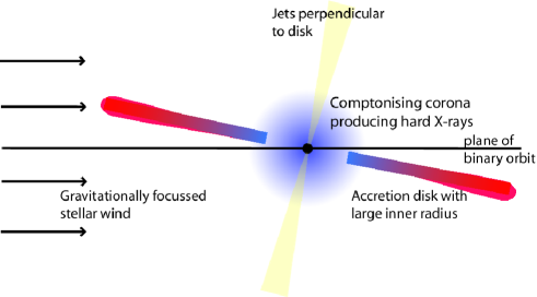
Figure 1: Likely geometry in the hard state of Cyg X-1. Mass being accreted forms an accretion disc around the compact object. In the inner regions, there is a hot inner flow/corona. Soft seed photons from the disc may be Comptonized in the hot flow. A fraction of the resulting hard photons can then be reflected off the disc, giving a net polarization.

Soft X-rays are produced in the accretion disc, and may then be Comptonized in the hot inner flow/corona. A fraction of the hard radiation can be reflected off the accretion disc before reaching the observer. Polarization from this system may arise through several processes. In this paper, we will focus on the polarization introduced by the reflection (for more details, see, e.g., [19, 25, 26]). In Cygnus X-1, this contribution is strongest in the energy range of $\sim$ 20–100 keV. The polarization degree is expected to vary with energy, following the relative strength of the reflection component.

1.2.2 Accreting magnetic neutron stars

In many high-mass XRBs the accreting object is a highly magnetic neutron star. The strong magnetic field, $\sim 10^{13}$ gauss at the surface, directs the accretion flow towards the magnetic poles of the star. Most of the accretion energy is released just above the polar cap where the emission and propagation of radiation is directly connected to the magnetic field as well as the local properties of the plasma. For a number of sources cyclotron spectral features have been observed in hard X-rays, and from these, magnetic field strengths have been deduced. The X-rays are expected to be polarized and the degree, angle and energy dependence of the polarization will depend on the physical conditions in the emission region [27]. Measurements of the detailed polarization properties would therefore provide a new and very powerful probe of the radiating plasma near the surface of the neutron star.

2 The Compton technique

Apart from the special case of Bragg reflection, all three main physical processes of photon-matter interaction in the X/$\gamma$-ray regime may be used in polarimetry: photoabsorption, Compton scattering and pair production. Each of these preserves information on the polarization of the incoming radiation. For photon energies between $\sim 100$ keV and 1 MeV, Compton scattering is the dominant process. In this section, we will briefly outline the theoretical basis for a polarimeter based on Compton scattering, and present a design for a dedicated polarimeter based on this technique.

2.1 Basic principle

The differential cross section for Compton scattering is given by:

$$\frac{\textrm{d}{\sigma_{\rm cs}}}{\textrm{d}{\Omega}}=\frac{1}{2}r_{e}^{2}\frac{E^{2}}{E_{0}^{2}}\left[\frac{E}{E_{0}}+\frac{E_{0}}{E}-2\sin^{2}\theta\cos^{2}\phi\right]\>,$$ (1)

where $r_{e}$ is the classical electron radius, $E_{0}$ and $E$ are the photon frequency before and after scattering, $\theta$ is the angle between incident and scattered direction, and $\phi$ is the azimuthal scattering angle relative to the plane of polarization. When projected on a plane, the angle of scattering will thus be modulated as $\cos^{2}\phi$.

To measure the scattering angles, it is necessary to detect both the site of scattering and that of photoabsorption. If more than two scattering sites are identified, the relative energy depositions can be used to help distinguish between Compton scattering and photoelectric absorption sites. Some form of segmentation of the detector is necessary to provide spatial resolution, required to determine the positions of the signals.

2.2 PoGOLite

The Polarized Gamma-ray Observer - Light weight version (PoGOLite) is a balloon-borne polarimeter, planned for launch with a stratospheric balloon in 2009. Figure 2 shows the design of the instrument.

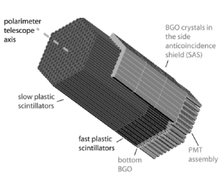
Figure 2: The design of the PoGOLite instrument. The side anticoincidence shield has been partially cut away for clarity. The total length of the instrument will be $\sim 100$ cm.

The instrument consists of 217 phoswich detector cells (PDCs) arranged in a hexagonal pattern. Each PDC is made up of a hollow slow scintillator tube, a fast scintillator detector, a bottom bismuth germanate (BGO) crystal, and a photomultiplier tube (PMT). Signals from the different optical components are distinguished using a pulse shape discrimination technique based on the different scintillation decay times of the materials [28]. The configuration is surrounded by an anticoincidence shield made of BGO crystals. Together with the bottom BGO crystals, this allows side and back entering photons and cosmic rays to be rejected.

The hollow slow scintillator tube acts as an active collimator. Photons or charged particles entering the instrument off-axis will be registered in the slow scintillator and can be rejected. The desired events are from photons that enter cleanly through the slow scintillator and scatter in the fast scintillator. After scattering, the photon may be absorbed in one of the neighbouring fast scintillator cells, allowing the azimuthal scattering angle to be determined.

The well-type design of PoGOLite allows for efficient background rejection [29, 30], and gives a field of view of $\sim 5\;{\rm deg}^{2}$. This allows the instrument to be accurately pointed at specific sources. As both the initial Compton scattering and subsequent photon absorption occur in the same material (the plastic fast scintillator), the effective energy range is determined by the cross-sections for both these processes, as well as the background. PoGOLite will have an energy range of $\sim$ 25–100 keV, which is lower than the range where Compton scattering dominates. A more detailed description of the instrument may be found in [28, 31].

The capability of PoGOLite to measure the energy dependence of polarization is limited both by the signal-to-background ratio and the energy resolution. Due to redistribution, some of the higher energy photons will produce events at lower energies. The flux and polarization in the low energy band will therefore be affected by the spectrum at higher energies but not vice-versa. The energy response has been carefully simulated using Geant4 [32].

Figure 3: Simplified sketch of the distribution of scattering angles, used to determine the modulation factor. The maximum ($C_{\rm max}$), minimum ($C_{\rm min}$) and average ($T=[C_{\rm max}+C_{\rm min}]$/2) values of the distribution are indicated.

Figure 3 shows a hypothetical distribution of azimuthal scattering angles. The maximum ($C_{\rm max}$) and minimum ($C_{\rm min}$) values of the distribution and the average ($T=[C_{\rm max}+C_{\rm min}]$/2) can be used to define a modulation factor:

$$M\equiv\frac{C_{\rm max}-C_{\rm min}}{C_{\rm max}+C_{\rm min}}=\frac{C_{\rm max}-C_{\rm min}}{2T}\;.$$ (2)

The modulation factor is determined by fitting the following function to the distribution of azimuthal scattering angles

$$f(x)=T(1+M\cos(2x+2\alpha))\>,$$ (3)

with angle $x$ (a function variable, not a fitting parameter), average $T$, modulation factor $M$, and polarization angle $\alpha$.

In this work, the modulation factor is the discriminator between different polarization models. If the response of the instrument to a 100% polarized source is known, the modulation factor can be used to determine the polarization of the incoming photon beam [33].

3 Simulations

In this section we will describe the setup of our simulations. The source models used as input are also presented, as well as the background considered.

3.1 Geant4

Geant4 is a multi-purpose software package for simulating particles travelling through and interacting with matter, using Monte Carlo techniques [34]. The standard Geant4 package was earlier found [35] to have incorrect implementations concerning photon polarization in Compton and Rayleigh scattering; the Geant4 version used here is a corrected version of 4.8.0.p01.

3.2 Simulation setup

The Geant4 implementation includes the essential parts of PoGOLite: 217 PDCs with slow and fast plastic scintillators and bottom BGO crystals together with a BGO side shield. The model has no PMTs, and uses a solid BGO side shield instead of discrete pentagonal bars (cf. Fig. 2). Layers of tin (50$\,\mu$m) and lead (50$\,\mu$m) surrounding each slow scintillator and the ${\rm BaSO_{4}}$ coating (200$\,\mu$m) of the BGO crystals are included. The mechanical support structure is not represented.

During the simulation, separate photons are generated with random energies from a spectral model. An event is triggered by a hit in two or three of the fast plastic scintillators. The following is saved as output data for each event: information about the original gamma momentum, the ID-number of the cells that had an interaction (ranging from 1 to 217) and the energy deposited in each cell. These data are preprocessed to simulate the resolution of the PMTs, as described in Sect. 4.1.

3.3 Source Models

As stated in Sect. 1.2, two sources were considered: Cygnus X-1 (in the hard state) and an accreting neutron star. Below we describe the model used for the incident radiation and polarization in each case. As shown in [10], PoGOLite is expected to detect polarization in both these sources; what we are investigating is the sensitivity to changes in polarization degree with energy.

3.3.1 Cygnus X-1

For our simulations of Cygnus X-1 we used an input spectrum of a power-law, with photon index $\alpha=-1.2$ and an exponential cutoff at energy $E_{\rm cut}=120$ keV. It was normalised to match the observed spectrum of Cygnus X-1. The spectrum of the reflection was approximated by the logarithmic quadratic curve

$$EF_{E}=10^{-c(\log E-\log a)(\log E-\log b)},$$ (4)

with $a=24$, $b=98$ and $c=1.89$. Figure 4 shows the observed radiation of Cygnus X-1, and our model of the total spectrum as well as that assumed for the reflection component.

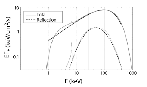
Figure 4: Observed radiation spectrum and input model used in the simulations of observations of Cygnus X-1. Gray lines: Typical radiation spectrum of Cygnus X-1 in the hard state. Black lines: Assumed input spectrum: a cut-off power law with index $\alpha=-1.2$ and cut-off $E_{\rm cut}=120$ keV, normalized to match the measured flux. The reflection component is shown, and the energy range of PoGOLite is indicated by vertical lines.

In our simulations, the polarization is assumed to arise due to the reflection component. Two scenarios were tested: 100% and 20% polarization for the reflection component, with unpolarized direct emission. This corresponds to a total average polarization around 17% and 3% respectively. The energy dependent polarization $\Pi(E)$ used as input was set to the relative strength of the reflection component compared to the total flux, scaled down in the case of 20% polarization. Simulations were performed for effective observing times of 6 hours and 35 hours. These times are chosen as realistic estimates for short and long duration balloon flights, respectively.

3.3.2 Accreting Magnetic Neutron Star

In the case of the neutron star, we study the observability of energy dependent effects by simulations of three different idealized polarized spectra:

• Polarization in a narrow band.

• Polarization only at low energies.

• Polarization only at high energies.

The neutron star spectrum was in all cases approximated with an exponentially cut-off power law, with index $\alpha=-1.1$ and energy cut-off at $E_{\rm cut}=70$ keV. It was normalized to correspond to a 100 mCrab source.

Assuming a cyclotron energy $E_{c}$ at 50 keV, we use three toy models of the polarization energy dependence $\Pi(E)$, with $\Pi_{\rm max}\equiv p\,\%$:

• A Gaussian peak centred at 50 keV, $G_{p}$, modelling a rise in polarization from 0% to maximum $p\,$%, using the Gaussian curve

  $$\Pi(E)=pe^{\frac{-(E-50)^{2}}{2\sigma^{2}}}\,\%$$ (5)

  with $E$ measured in keV and $\sigma=5$ keV.

• Two step functions, $S_{p}$ and $S_{-p}$, with polarization

  $$\Pi=\left\{\begin{array}[]{ll}0\%&\textrm{if $E<50$ keV}\\ p\,\%&\textrm{if $E\geq 50$ keV}\end{array}\right.$$ (6)

  for $S_{p}$, and

  $$\Pi=\left\{\begin{array}[]{ll}p\%&\textrm{if $E<50$ keV}\\ 0\,\%&\textrm{if $E\geq 50$ keV}\end{array}\right.$$ (7)

  for $S_{-p}$. Simply put, $p$ is the jump in polarization that occurs at $E=50$ keV.

Figure 5 illustrates examples of $G_{20}$ and $S_{10}$, the Gaussian and positive steps with maxima 20% and 10% respectively. In the simulations, the values $p=\{10,20,30,40,50\}$% were used, each assuming an observation time of 35 hours.

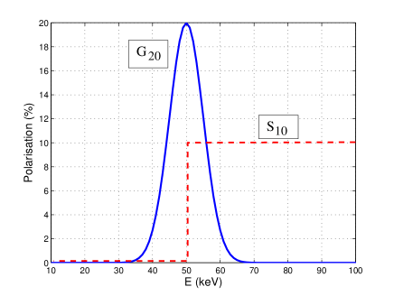
Figure 5: Example of assumed energy dependence of the polarization fraction in the case of an accreting magnetic neutron star. The figure shows a Gaussian curve with $\Pi_{\rm max}=20\%$ (G₂₀), and a positive step with $\Pi_{\rm max}=10\%$ (S₁₀).

3.4 Background

Balloon-borne gamma-ray polarimetry measurements are subject to several significant sources of background. Through the use of the well-type phoswich detector technique, the PoGOLite instrument has been designed to reduce these backgrounds, allowing 10% polarization of a 100 mCrab source to be measured in one 6 hour balloon observation in the 25–100 keV energy range. The basic phoswhich design was used in the WELCOME series of balloon-borne observations and allowed effective background suppression [36, 37, 38, 39, 40, 41, 42]. The concept was subsequently improved and effectively used in a satellite instrument, the Suzaku Hard X-ray Detector (HXD) [29, 43, 44, 45].

The background to PoGOLite measurements can arise from charged cosmic rays, neutrons (atmospheric and instrumental) and gamma-rays (primary and atmospheric). The background from charged cosmic rays (predominantly protons, $\sim$90%, and helium nuclei, $\sim$10%) is rejected by the BGO anticoincidence shields and slow plastic collimators. Cosmic rays are minimum ionizing particles and can be identified through their relatively large energy deposits. The background presented by atmospheric neutrons and neutrons produced in the PoGOLite instrument and surrounding structures is currently being studied in detail [46]. For the purposes of the study presented in this paper, particular attention has been paid to what is expected to be the dominant background: primary and atmospheric gamma-rays. The gamma-ray background rate is estimated from a model derived from measurements taken in Texas with the GLAST Balloon Flight Engineering Model [47].

The primary gamma-ray component originates outside the atmosphere, i.e., above PoGOLite. The angular distribution of the radiation is uniform within the hemisphere above PoGOLite. The energy spectrum is modeled by a doubly-broken power-law with breaks at 50 keV and 1 MeV [48].

Secondary gamma-rays are created in the Earth’s atmosphere through bremsstrahlung interactions of charged cosmic-rays. Two separate components are considered, one directed upwards and one downwards. The upward flux is dependent on the zenith angle [49], and the energy spectrum consists of a doubly-broken power-law with breaks at 10 MeV and 1 GeV, and a 511 keV line from electron-positron annihilation. The downward component is similar, but with breaks at 1 MeV and 1 GeV. Energies up to 100 GeV were generated for all components. These models are based on data from satellite- and balloon-borne instruments ([50] and [51], and references therein).

Figure 6 shows the estimated gamma-ray backgrounds compared to the accreting pulsar and Cygnus X-1 models. The total gamma-ray background is at the 10 mCrab level.

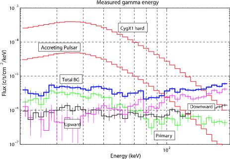
Figure 6: Estimated contribution to the gamma-ray background in the PoGOLite energy range ($\sim$ 25–100 keV). The radiation from the two considered sources, Cygnus X-1 and an accreting neutron star, are also shown.

4 Analysis and Results

4.1 Data Processing

In the first data processing step, the resolution of the scintillator-PMT assembly is simulated by fluctuating the number of photo-electrons generated in the scintillating materials. It is assumed that when the energy $E$ is deposited in a cell, the average number of photo-electrons generated is $En$, with $n$ set to 0.5 photo-electrons per keV. Now, we fluctuate $En$ to $(En)_{\rm fluct}$ by applying a Gaussian spread. If $En\leq 10$, we do it in two steps: First we subject it to a Poissonian spread, and thereafter a Gaussian spread with variance $En\sigma^{2}$, with $\sigma$ set to 0.4. If $En>10$, only a Gaussian spread with variance $En$ is used. If $(En)_{\rm fluct}<0$, then it is set to 0. Finally, we take

$$E_{\rm mes}=\frac{(En)_{\rm fluct}}{n}$$ (8)

as the energy actually measured by the PMT in the cell of interest. We reject all fast scintillator interactions with $E_{\rm mes}$ below a certain measurement threshold (2 keV). For the analysis described in this paper, only events with two or three hits in the fast scintillators are retained (the veto logic is not considered at this stage). At PoGOLite energies, more than 80% of the events are from photons interacting in no more than three detector cells [52].

For two-site events, the chronological order of the two cells does not matter for angle calculation, as the distribution is periodic over the angle $\pi$. In the case of three hits, we calculate the scattering angle by ignoring the hit with the lowest energy measured, assuming that a low-energy interaction does not affect direction much, and derive an angle from the positions of the two cells with highest energy deposits.

Most photons do not scatter very far; about half will only go from one cell to its neighbour. As the range of possible scattering angles resulting in detection in a given adjacent cell is large, this causes strong peaks in each of the six directions corresponding to the neighbouring cells. The PoGOLite instrument will rotate about its axis, causing the range for a given cell to smoothly vary and thereby creating a continuous distribution over angles. In the simulations, the uncertainty of the angle determination is instead approximated by introducing a Gaussian spread to the measured scattering angles.

In the last steps of data processing we take into account the mass of air in the atmosphere above the balloon, filtering out roughly half of our incident source radiation, assuming the atmospheric overburden 4 g/cm² at 40 km altitude. We also apply the veto logic, rejecting all events with detection in any slow plastic scintillator or BGO crystal.

4.2 A $\chi^{2}$ measure

To measure the polarization energy dependence, one cannot simply calculate the polarization at certain energies and construct $\Pi(E)$, since the photon energy $E_{\gamma}$ always will be unknown due to the response of the instrument. Instead we calculate the modulation factor at different measured energies, obtaining a curve $M(E_{\rm mes})$. This curve can then be compared with theoretic curves resulting from other models, possibly from the same family of curves, enabling us to reject complete families of energy dependencies. One such family, which we will be concerned with here, is the set of constant polarizations.

For a given source model (polarization energy dependence) A, the modulation factor $M$ (Eq. 2) was fitted at different measured energies, yielding a curve $M_{A}=M_{A}(E_{\rm mes})$. Figure 7 shows an example of a modulation curve in the 30–35 keV band, generated for a six hour observation of Cygnus X-1 in the case of a completely polarized reflection component. The resulting modulation factor is $2.69\pm 0.30$. The modulation factor is in this way calculated for each energy band. The result is a curve showing how the modulation factor varies with energy, which can then be compared to the corresponding curves for various models of polarization.

Figure 7: Example of the measured distribution of events as a function of scattering angle (histogram). In this example, the simulated results of a six hour observation of Cygnus X-1 are shown, assuming a completely polarized reflection component. The data are from the measured energy range of 30–35 keV. A sinusoidal function is fit to the data (solid line, cf. Eq. 3) and a modulation factor is calculated.

To test the results against constant polarization, we also generated curves $M_{\Pi}$ with constant levels of polarization $\Pi$. Since these latter curves should not be thought of as measured, but fluctuation-free theoretical constructs, they were generated by much longer simulations than the observational curves.

A measure of how much two curves differ is defined as

$$\chi^{2}_{\Pi}=\sum_{E_{\rm mes}}\frac{(M_{A,E_{\rm mes}}-M_{\Pi,E_{\rm mes}})^{2}}{\sigma_{E_{\rm mes}}^{2}},$$ (9)

with $\sigma_{i}$ as the sum of the two errors in fitting $M_{A,E_{\rm mes}}$ and $M_{\Pi,E_{\rm mes}}$. When this is calculated for all reasonable values of $\Pi$, we can reject the hypothesis of constant polarization if the minimum of $\chi^{2}_{\Pi}$ is high enough. For 16 degrees of freedom, corresponding to data points up to 100 keV, the 95% certainty level requires $\chi^{2}>26.3$.

4.3 Cygnus X-1

Table 1 summarises the results for the simulations of Cygnus X-1. For a 100% polarized reflection component, the energy dependence is detected both after 6 hours of observation and after 35 hours. Figure 8 shows the expected modulation factors and $\chi^{2}$ values for a 35h observation. In the case of 20% polarization of the reflection component, shown in Fig. 9, constant polarization cannot be ruled out at any higher significance level.

	Reflection 100%		Reflection 20%
Obs. time	6h	35h	6h	35h
Significance	99.4%	$>$99.99%	19.1%	51.2%

Table 1: The significance in rejecting constant polarization models, shown for different reflection polarization strengths and observation times in the case of Cygnus X-1.

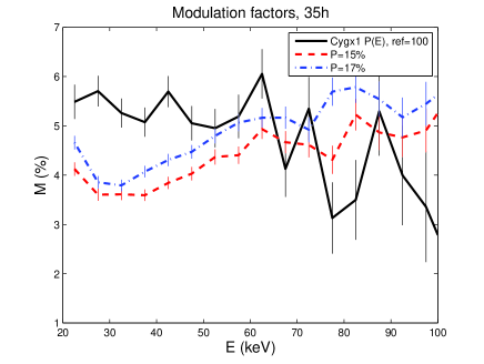
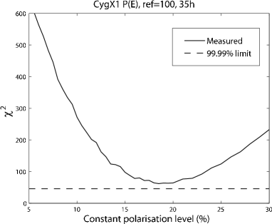
Figure 8: Results from simulations of a 35h observation of Cygnus X-1, with the reflection component assumed to be 100% polarized. Left panel: Expected modulation factor $M(E)$, together with models of constant polarization at 15% and 17%. The modulation is fitted in intervals of 5 keV. Right panel: $\chi^{2}$ values when comparing $M(E)$ for the simulation with different degrees of constant polarization. The dashed line marks the limit for 99.9% significance in rejecting constant polarization. Constant polarization is rejected with high significance.

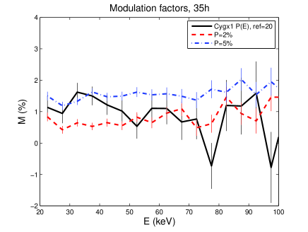
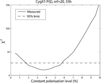
Figure 9: Same as Fig. 8, but with the reflection component assumed to be 20% polarized. Left panel: Expected modulation factor $M(E)$, together with models of constant polarization at 2% and 5%. Right panel: $\chi^{2}$ values when comparing $M(E)$ for the simulation with different degrees of constant polarization. The dashed line marks the limit for 95% significance in rejecting constant polarization. Constant polarization cannot be rejected with high significance.

4.4 Magnetic NS

The results for the simulations of the accreting neutron star are summarised in Table 2. For a 100 mCrab source, the background will start to become significant already in the higher end of the PoGOLite energy range. To be conservative, only $M(E)$ data points up to 60 keV were used for the $\chi^{2}$ analysis in order to limit the errors due to uncertainties in the background flux. This is equivalent to 8 degrees of freedom, demanding $\chi^{2}>15.5$ for 95% certainty in rejecting constant polarization.

Gaussian peaks
$\Pi_{\textrm{max}}$ (%)	10	20	30	40	50
Significance	24.3%	24.3%	35.3%	79.9%	99.7%
Positive steps
$\Pi_{\textrm{max}}$ (%)	10	20	30	40	50
Significance	46.3%	70.0%	96.8%	91.8%	83.5%
Negative steps
$\Pi_{\textrm{max}}$ (%)	10	20	30	40	50
Significance	51.0%	99.3%	95.8%	99.6%	$>$99.99%

Table 2: The significance in rejecting constant polarization models, shown for different polarization shapes and maxima in the case of a 100 mCrab neutron star.

4.4.1 Gaussian peaks

In Fig. 10 we see $M(E)$ curves for $G_{50}$ and a few constant polarizations (left panel), clearly illustrating their different characteristics. The resulting $\chi^{2}$ curve (right panel) confirms that these models are significantly (99% level) different. However, this was not the case for any lower value of $\Pi_{\rm max}$.

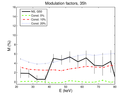
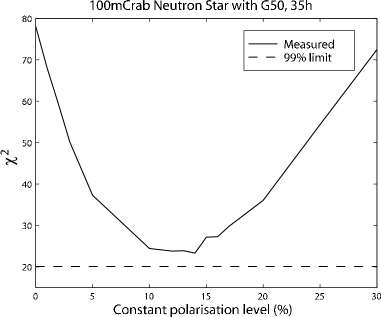
Figure 10: Results from simulations of a 35h observation of an accreting magnetic neutron star, assuming a Gaussian polarization curve. Left panel: Expected modulation factor $M(E)$, together with models of constant polarization at 0%, 10% and 20%. The modulation is fitted in intervals of 5 keV. Right panel: $\chi^{2}$ values when comparing $M(E)$ for the simulation with different degrees of constant polarization. The dashed line marks the limit for 95% significance in rejecting constant polarization. Constant polarization is rejected with high significance.

4.4.2 Positive steps

Figure 11 shows the result for $S_{50}$ when compared to cases of constant polarization. In this case, the difference in characteristics between the constant models and the energy dependent model is not large enough, and constant polarization cannot be ruled out. The only value of $\Pi_{\rm max}$ yielding a significant (95% level) difference was $\Pi_{\rm max}=30\%$. What is interesting to note is that a higher $\Pi_{\rm max}$, which implies a higher total polarization, does not necessarily make the energy dependence easier to measure.

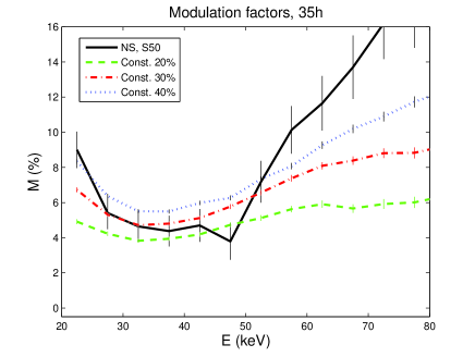
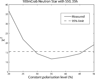
Figure 11: Results from simulations of a 35h observation of an accreting magnetic neutron star, assuming a positive step with $\Pi_{\rm max}=50\%$. Left panel: Expected modulation factor $M(E)$, together with models of constant polarization at 20%, 30% and 40%. The modulation is fitted in intervals of 5 keV. Right panel: $\chi^{2}$ values when comparing $M(E)$ for the simulation with different degrees of constant polarization. The dashed line marks the limit for 95% significance in rejecting constant polarization. Constant polarization cannot be rejected with high significance.

4.4.3 Negative steps

The result of the $S_{-50}$ model is shown in Fig. 12, where the $\chi^{2}$ plot (right panel) allows us to reject constant polarization with a certainty much higher than 99.99%. Other models yielding significant detections were $S_{-20}$ (99%), $S_{-30}$ (95%), and $S_{-40}$ (99%). One reason these models are so easily measurable stems from the fact that, due to the shape of the neutron star spectrum, data and statistics are much poorer at higher energies. If the polarized part only lies at high energies, the total polarization will be much lower or even undetectable.

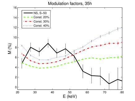
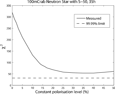
Figure 12: Same as in Fig. 11, but using the negative step. In this case, constant polarization is rejected with high significance.

5 Discussion

Although no measurements have been made of polarization in the energy range covered by PoGOLite, some theoretical models predict changes in polarization with energy. The results of the simulations clearly show that it is possible for the PoGOLite instrument to detect the energy dependence of polarization for several of the investigated cases. The highest significance is found for Cygnus X-1 assuming a fully polarized reflection component and a neutron star in the case of a negative step; in the remaining cases, constant polarization can not be rejected. Our results therefore show that PoGOLite has the potential to discriminate among these models.

As described above, in Cygnus X-1 the hard X-rays are believed to originate from Comptonization of soft seed photons in a predominantly thermal electron distribution. Although this process involves Compton scattering – which could introduce a net polarization – multiple scatterings are required, making our assumption of the direct component being unpolarized a reasonable one. The degree of polarization of the reflected component is however more uncertain. Our idealized case of 100% polarization is certainly an overestimation. Calculations [19] show that the degree of polarization in the reflected component varies with inclination, with a maximum of $\sim 30\%$ expected at high inclination. The inclination of the Cygnus X-1 system is not well known, but estimates put it at $30^{\circ}$–$50^{\circ}$ [53], making our assumption of 20% polarization in the reflected component reasonable. The relative size of the reflected component compared to the direct emission is in turn dependent on both inclination, where the dependence is the opposite one, and system geometry. We note that in other sources the reflected component may be much stronger, or even dominate the radiation spectrum (e.g., Cygnus X-3, [54]).

Another issue which may complicate measurements of energy dependent polarization is the behaviour of the angle of polarization. In our simulations, we have implicitly assumed that the angle does not vary with energy. However, for both black hole and neutron star systems, this assumption may be an oversimplification. It is certainly true that emission originating from the region close to a black hole will be affected by the strong gravity, affecting the polarization angle [21]. It is not clear how large this effect would be on the reflected component in, for instance, Cygnus X-1, but results from both temporal and spectral analysis show that the accretion disc – assumed to be the reflector – is presumably truncated at a large distance ($R_{\rm in}\gtrsim 30R_{g}$, [55, 56]) from the black hole in the hard state. We therefore do not expect this effect to alter the outcome of our simulations.

Our results from simulating Cygnus X-1 indicate that long observations with PoGOLite are required to search for energy dependence of polarization. The first flights of the instrument will likely be shorter flights, covering several targets. While these observations should be long enough to detect polarization down to the level of a few per cent, we do not expect to detect any changes in polarization with energy. However, long duration flights spanning several days are also planned, and such flights would provide the observation time needed to search for variations of polarization degree with energy.

A point to note from the neutron star simulations is the result that it is easier to rule out constant polarization in the case of a negative step than for a positive step. As noted in Sect. 4, the energy response of the instrument is such that the energy of the incoming photon cannot be uniquely determined. The result will be a redistribution of energy, with a possibility for higher energy photons to be detected with lower energies. The reverse is however not true – a low energy photon will not be detected as having a higher energy. In the case of a positive step, some polarized high energy photons will be detected at lower energies. This will give a false polarization signal at lower energies, and act to “smooth” the detected energy dependance of polarization. For a negative step, the polarization is introduced at lower energies and will not “spread” to higher energies. The low energy polarization will be somewhat diluted by redistribution of high energy photons but the polarization contrast will still be higher than in the positive case.

By excluding energies above 60 keV in the ${\chi}^{2}$ analysis of accreting X-ray pulsars we have been fairly conservative in our estimate of significances. The restriction of the energy range was motivated by a potentially high sensitivity to systematic errors in the background level at high energies. In this analysis however, we have not taken advantage of the fact that these sources are pulsating. By analysing the polarization of the pulsed flux, rather than the total flux, it should be possible to include all points up to 100 keV and thereby increase the sensitivity. On the other hand the polarization direction will probably change over the pulsation period which will have the opposite effect of reducing the sensitivity. How important this effect is depends on the precise source geometry, radiation beaming and our viewing angle.

As PoGOLite’s field-of-view is rather large ($\sim 5\;{\rm deg}^{2}$), the pointing errors with respect to the axis of rotation must be small to avoid introducing systematic errors in the polarization measurements. The attitude control system used for PoGOLite will assure accurate pointing to within a few arcminutes, keeping the systematic error below 1% [10]. Although this figure refers to the whole energy band, we do not expect any such effect to change the results presented here. A comprehensive study of systematic effects is beyond the scope of this paper, but will be crucial once PoGOLite is in operation.

The performance of the PoGOLite instrument has been extensively evaluated, both with laboratory-based tests [57], accelerator-based tests [28], and simulations [32]. These tests show that it will be able to detect low ($\sim 10\%$) degrees of polarization even for 100 mCrab sources. What has not previously been tested is its sensitivity to a polarization degree that varies with energy. Despite the relatively modest inherent energy resolution, our results show that PoGOLite has the capacity to detect changes in polarization degree with energy. The simulations show that significant results can be obtained in a 35h observation, attainable in the long duration flights already planned for PoGOLite. We stress that the design is not optimized for such detections, and future instruments will in all likelihood develop this technique further.

6 Conclusions

The Compton technique applied to an array of plastic scintillators is an effective method to measure broad energy band polarization, which is demonstrated with the proposed PoGOLite mission, using Geant4 simulations. In particular, energy dependence can be detected. However, in our model of polarization from X-ray binaries, we require the reflection to contribute a large fraction of the observed flux and/or have high degree of polarization for energy dependence to be detected. Similarly, for accreting magnetic neutron stars, sharp energy variations in the polarization are needed for a clear detection. This is made easier if the lower energies contain most of the polarization.

References

- [1] J. Tinbergen, Astronomical Polarimetry, Cambridge University Press (2005)
- [2] R. Novick, M. C. Weisskopf, R. Berthelsdorf, R. Linke, & R. S. Wolff, Astrophys. J. Lett. 174 (1972), L1
- [3] M. C. Weisskopf et al, Astrophys. J. Lett 208 (1976), L125
- [4] M. C. Weisskopf, E. H. Silver, H. L. Kestenbaum, K. S. Long, & R. Novick, Astrophys. J. Lett. 220 (1978), L117
- [5] N. Produit, et al., Nucl. Instr. and Meth. A 550 (2005), 616
- [6] J. Legere, et al., Proc. SPIE 5898 (2005), 413
- [7] S. Gunji et al., Proc. ICRC (2003), 2779
- [8] R. Silva, et al., Proc. SPIE 4843 (2003), 543
- [9] E. Costa et al., 2006, astro-ph/0609576
- [10] T. Kamae, et al., A&A, in preparation
- [11] M. J. Rees, Mon. Not. R. Astron. Soc. 171 (1975), 457
- [12] P. Meszaros, R. Novick, A. Szentgyorgyi, G. A. Chanan, & M. C. Weisskopf, Astrophys. J. 324 (1988), 1056
- [13] E. Agol, & O. Blaes, Mon. Not. R. Astron. Soc. 282 (1996), 965
- [14] G. Matt, Astron. Astrophys. 423 (2004), 495
- [15] K. Viironen, & J. Poutanen, Astron. Astrophys. 426 (2004), 985
- [16] K. C. Westfold, Astrophys. J. 130 (1959), 241
- [17] I. N. Gnedin & R. A. Sunyaev, A&A 36 (1974), 379
- [18] R. A. Sunyaev, & L. G. Titarchuk, Astron. Astrophys. 143 (1985), 374
- [19] G. Matt, Mon. Not. R. Astron. Soc. 260 (1993), 663
- [20] J. Ogura, N. Ohuo, & Y. Kojima, Publ. Astron. Soc. Jap. 52 (2000), 841
- [21] P. A. Connors, R. F. Stark, & T. Piran, Astrophys. J. 235 (1980), 22
- [22] V. Karas, M. Dovciak, & G. Matt, ArXiv Astrophysics e-prints (2005), arXiv:astro-ph/0501579
- [23] R. Novick, M. C Weisskopf, J. R. P. Angel, & P. G. Sutherland, Astrophys. J. Lett. 215 (1977), L117
- [24] J. Poutanen, in Theory of Black Hole Accretion Disks, edited by M. A. Abramowicz, G. Björnsson, and J. E. Pringle. Cambridge University Press, 1998, p.100
- [25] G. Matt, A. C. Fabian, & R. R. Ross, Mon. Not. R. Astron. Soc. 264 (1993), 839
- [26] D. R. Ballantyne, R. R. Ross, & A. C. Fabian, Mon. Not. R. Astron. Soc. 327 (2001), 10
- [27] V. Andersson et al., in Proc. 22nd Texas Symposium on Relativistic Astrophysics, Stanford, Dec. 13-17, 2004.
- [28] Y. Kanai, et al., Nucl. Instrum. Methods Phys. Res. A 570 (2007), 61
- [29] T. Kamae et al., SPIE 2806 (1996), 314
- [30] T. Takahashi et al., SPIE Vol. 1734 (1992), 2
- [31] S. Larsson, & M. Pearce, Nucl. Instrum. Methods Phys. Res. A 525 (2004), 148
- [32] O. Engdegård, Studies of Energy Dependent X-ray Polarisation with PoGOLite - Monte Carlo Simulations with Geant4, Master’s thesis (2006), http://www.particle.kth.se/pogolite
- [33] F. Lei, et al., Space Sci. Rev. Vol 82 (1997), 309
- [34] S. Agostinelli et al., Nucl. Instrum. Methods Phys. Res. A 506 (2003), 250
- [35] T. Mizuno et al., Nucl. Instrum. Methods Phys. Res. A 540 (2005), 158
- [36] T. Kamae et al., SPIE 1734 (1992), 2
- [37] T. Kamae et al., IEEE Trans. Nucl. Sci. 40(2)(1993), 204
- [38] T. Takahashi et al., IEEE Trans. Nucl. Sci. 40(3) (1993), 890
- [39] S. Gunji et al., Astrophys. J. 397 (1992), L83
- [40] S. Gunji et al., Astrophys. J. 428 (1994), 284
- [41] S. Miyazaki et al., Publ. Astron. Soc. Jap. 48 (1996), 801
- [42] N. Yamasaki et al., Astrophys. J. 481 (1997), 821
- [43] K. Makishima et al., ASP Conf. Proc. 251 (2001) Eds. H. Inoue and H. Kunieda, 564
- [44] M. Kokubun et al., IEEE Trans. Nucl. Sci. 51 (2004), 1991
- [45] Suzaku AO document (2005), posted at http://heasarc.gsfc.nasa.gov/docs/astroe/prop_tools/suzaku_td/
- [46] J. Kazejev, Master’s Thesis, Royal Institute of Technology (in preparation).
- [47] T. Mizuno et al., Astrophys. J. 614 (2004), 1113
- [48] P. Sreekumar et al., Astrophys. J. 494 (1998), 523
- [49] V. Schönfelder, et al., Astrophys. J. 217 (1977), 306
- [50] N. Gehrels, Nucl. Instr. and Meth. A 239 (1985), 324
- [51] V. Schönfelder, F. Graml, & F. P. Penningsfeld, Astrophys. J. 240 (1980) 350
- [52] M. Kiss, M. Pearce, PoGOLite: Opening a new window on the universe with polarized gamma-rays, proc. for Imaging 2006 conf. (2007), in press
- [53] J. M. Miller et al., Astrophys. J. 578 (2002), 348
- [54] L. Hjalmarsdotter et al., submitted to Mon. Not. R. Astron. Soc.
- [55] M. Axelsson, L. Borgonovo, & S. Larsson, Astron. Astrophys. 452 (2006), 975
- [56] M. Gierlinski et al., Mon. Not. R. Astron. Soc. 288 (1997), 958
-
[57]
M. Kiss, Construction and laboratory tests of the PoGO-Lite prototype, Master’s thesis (2006)
http://www.particle.kth.se/pogolite