The VIMOS VLT Deep Survey

We present a detailed analysis of the Galaxy Stellar Mass Function (GSMF) of galaxies up to $z=2.5$ as obtained from the VIMOS VLT Deep Survey (VVDS). Our survey offers the possibility to investigate it using two different samples: (1) an optical ($I$-selected $17.5<I_{\rm AB}<24$) main spectroscopic sample of about 6500 galaxies over 1750 arcmin² and (2) a near-IR ($K$-selected $K_{\rm AB}<22.34\leavevmode\nobreak\ \&\leavevmode\nobreak\ K_{\rm AB}<22.84$) sample of about 10200 galaxies, with photometric redshifts accurately calibrated on the VVDS spectroscopic sample, over 610 arcmin². We apply and compare two different methods to estimate the stellar mass ${\cal M}_{\rm stars}$ from broad-band photometry based on different assumptions on the galaxy star-formation history. We find that the accuracy of the photometric stellar mass is overall satisfactory, and show that the addition of secondary bursts to a continuous star formation history produces systematically higher (up to 40%) stellar masses. We derive the cosmic evolution of the GSMF, the galaxy number density and the stellar mass density in different mass ranges. At low redshift ($z\simeq 0.2$) we find a substantial population of low-mass galaxies ($<10^{9}M_{\odot}$) composed by faint blue galaxies ($M_{I}-M_{K}\simeq 0.3$). In general the stellar mass function evolves slowly up to $z\sim 0.9$ and more significantly above this redshift, in particular for low mass systems. Conversely, a massive population is present up to $z=2.5$ and have extremely red colours ($M_{I}-M_{K}\simeq 0.7-0.8$). We find a decline with redshift of the overall number density of galaxies for all masses ($59\pm 5$% for ${\cal M}_{\rm stars}>10^{8}M_{\odot}$ at $z=1$), and a mild mass-dependent average evolution (‘mass-downsizing’). In particular our data are consistent with mild/negligible ($<30$%) evolution up to $z\sim 0.7$ for massive galaxies ($>6\times 10^{10}M_{\odot}$). For less massive systems the no-evolution scenario is excluded. Specifically, a large fraction ($\geq 50\%$) of massive galaxies have been already assembled and converted most of their gas into stars at $z\sim 1$, ruling out the ‘dry mergers’ as the major mechanism of their assembly history below $z\simeq 1$. This fraction decreases to $\sim 33\%$ at $z\sim 2$. Low-mass systems have decreased continuously in number density (by a factor up to $4.1\pm 0.9$) from the present age to $z=2$, consistently with a prolonged mass assembly also at $z<1$. The evolution of the stellar mass density is relatively slow with redshift, with a decrease of a factor $2.3\pm 0.1$ at $z=1$ and about $4.5\pm 0.3$ at $z=2.5$.

1 Introduction

One of the main and still open question of modern cosmology is how and when galaxies formed and in particular when they assembled their stellar mass. There are growing but still controversial evidences in near-IR (NIR) surveys that luminous and rather massive old galaxies were quite common already at $z\sim 1$ (Pozzetti et al. 2003, Fontana et al. 2004, Saracco et al. 2004, 2005, Caputi et al. 2006a) and up to $z\sim 2$ (Cimatti et al. 2004, Glazebrook et al 2004). These surveys indicate that a significant fraction of early-type massive galaxies were already in place at least up to $z\sim 1$. Therefore they should have formed their stars and assembled their stellar mass at higher redshifts. As in the local universe, at $z\simeq 1.5$ these galaxies still dominate the near-IR luminosity function and stellar mass density of the universe (Pozzetti et al. 2003, Fontana et al. 2004, Strazzullo et al. 2006). These results favour a high-$z$ mass assembly, in particular for massive galaxies, in apparent contradiction with the hierarchical scenario of galaxy formation, applied to both dark and baryonic matter, which predicts that galaxies form through merging at later cosmic time. In these models massive galaxies, in particular, assembled most of their stellar mass via merging only at $z<1$ (De Lucia et al. 2006). From several observations it seems that baryonic matter has a mass-dependent assembly history, from massive to small objects, (i.e. the ‘downsizing’ scenario in star formation, firstly defined by Cowie et al. 1996, is valid also for mass assembly), opposite to the dark matter (DM) halos assembly. The continuous merging of DM halos in the hierarchical models, indeed, should result in an ‘upsizing’ in mass assembly, with the most massive galaxies being the last to be fully assembled. If we trust the hierarchical $\Lambda$CDM universe, the source of this discrepancy between observations and simple basic models could be due to the difficult physical treatment of the baryonic component, such as the star formation history/timescale, feedback, dust content, AGN feedback or to a missing ingredient in the hierarchical models of galaxy formation (for the inclusion of AGN feedback, see Bower et al. 2006, Kang et al. 2006, De Lucia & Blaizot 2007, Menci et al. 2006, Monaco et al. 2006; and see Neistein et al. 2006 for the description of a natural downsizing in star formation in the hierarchical galaxy formation models and a recent review by Renzini 2007).

Considering optically selected surveys, a strong number density evolution of early type galaxies has been recently reported from the COMBO17 and DEEP2 surveys (Bell et al. 2004, Faber et al. 2005), with a corresponding increase by a factor 2 of their stellar mass since $z\sim 1$, possibly due to so called ‘dry-mergers’ (even if the observational results on major merging and dry-merging are still contradictory, see Bell et al. 2006, van Dokkum 2005, Lin et al. 2004 and Renzini 2007 for a summary). This is at variance with results from the VIMOS-VLT Deep Survey (VVDS, Le Fèvre et al. 2003b ), conducted at greater depth and using spectroscopic redshifts in a large contiguous area. From the VVDS, Zucca et al. (2006) found that the $B$-band luminosity function of early type galaxies is consistent with passive evolution up to $z\sim 1.1$, while the number of bright ($M_{B_{AB}}<-20$) early type galaxies has decreased only by $\sim 40$% from $z\sim 0.3$ to $z\sim 1.1$. Similarly, Brown et al. (2007), in the NOAO Deep Wide Field survey over $\sim 10$ deg², found that the $B$-band luminosity density of $L^{*}$ galaxies increases by only $36\pm 13\%$ from $z=0$ to $z=1$ and conclude that mergers do not produce rapid growth of luminous red galaxy stellar masses between $z=1$ and the present day.

The VVDS is very well suited for this kind of studies, thanks to its depth and wide area, covered by multi-wavelength photometry and deep spectroscopy. The simple $17.5<I_{AB}<24$ VVDS magnitude limit selection is significantly fainter than other complete spectroscopic surveys and allows the determination of the faint and low mass population with unprecedented accuracy. Most of the previous existing surveys are instead very small and/or not deep enough, or based only on photometric redshifts.

Given the still controversial results based on morphology or colour-selected early-type galaxies (see Franzetti et al. 2007 for a discussion on colour-selected contamination), we prefer to study the total galaxy population using the stellar mass content. Here we present results on the cosmic evolution of the Galaxy Stellar Mass Function (GSMF) and mass density to $z=2.5$ in the deep VVDS spectroscopic survey, limited to $17.5<I_{\rm AB}<24$, over $\sim 1750$ arcmin² and based on about 6500 galaxies with secure spectroscopic redshifts and multiband (from UV to near-IR) photometry. In addition, we derive the GSMF also for a $K$-selected sample based on about 6600 galaxies ($K_{\rm AB}<22.34$) in an area of 442 arcmin² and about 3600 galaxies in a deeper ($K_{\rm AB}<22.84$) smaller area of 168 arcmin², making use of photometric redshifts, accurately calibrated on the VVDS spectroscopic sample, and spectroscopic redshifts when available.

Throughout the paper we adopt the cosmology $\Omega_{m}=0.3$ and $\Omega_{\Lambda}=0.7$, with $h_{70}=H_{0}/70$ km s^-1 Mpc^-1. Magnitudes are given in the AB system and the suffix AB will be dropped from now on.

2 The First Epoch VVDS Sample

The VVDS is an ongoing program aiming to map the evolution of galaxies, large scale structures and AGN through redshift measurements of $\sim 10^{5}$ objects, obtained with the VIsible Multi-Object Spectrograph (VIMOS, Le Fèvre et al. 2003a ), mounted on the ESO Very Large Telescope (UT3), in combination with a multi-wavelength dataset from radio to X-rays. The VVDS is described in detail in Le Fèvre et al. (vvds1 (2005)). Here we summarize only the main characteristics of the survey.

The VVDS is made of a wide part, with spectroscopy in the range $17.5\leq I\leq 22.5$ on 4 fields ($\sim 2\times 2$ deg² each), and a deep part, with spectroscopy in the range $17.5\leq I\leq 24$ on the field 0226-04 (F02 hereafter). Multicolour photometry is available for each field (Le Fèvre et al. photom1 (2004)). In particular, the $B$, $V$, $R$, $I$ photometry for the 0226-04 deep field, covering $\sim 1$ deg², has been obtained at CFHT and is described in detail in McCracken et al. (photom2 (2003)). The photometric depth reached in this field is 26.5, 26.2, 25.9, 25.0 (50% completeness for point-like sources), respectively in the $B$, $V$, $R$, $I$ bands. Moreover, $U<25.4$ (50% completeness) photometry obtained with the WFI at the ESO-2.2m telescope (Radovich et al. photomU (2004)) and $K_{s}$ band (hereafter $K$) photometry with NTT+SOFI at the depth (50% completeness) of 23.34 (Temporin et al. in preparation) are available for wide sub-areas of this field. Moreover, an area of about $170$ arcmin² has been covered by deeper $J$ and $K$ band observations with NTT+SOFI at the depth (50% completeness) of 24.15 and 23.84, respectively (Iovino et al. photomK (2005)). The deep F02 field has been observed also by the CFHT Legacy Survey (CFHTLS) in several optical bands ($u^{*}$, $g^{\prime}$, $r^{\prime}$, $i^{\prime}$, $z^{\prime}$) at very faint depth ($u^{*}=26.4,g^{\prime}=26.3,r^{\prime}=26.1,i^{\prime}=25.9,z^{\prime}=24.9$, 50% completeness).

Spectroscopic observations of a randomly selected subsample of objects in an area of $\sim 0.5$ deg², with an average sampling rate of about 25%, were performed in the F02 field with VIMOS at the VLT.

Spectroscopic data were reduced with the VIMOS Interactive Pipeline Graphical Interface (VIPGI, Scodeggio et al. vipgi (2005), Zanichelli et al. ifu (2005)) and redshift measurements were performed with an automatic package (KBRED) and then visually checked. Each redshift measurement was assigned a quality flag, ranging from 0 (failed measurement) to 4 (100% confidence level); flag 9 indicates spectra with a single emission line, for which multiple redshift solutions are possible. Further details on the quality flags are given in Le Fèvre et al. (vvds1 (2005)).

The analysis presented in this paper is based on the first epoch VVDS deep sample, which has been obtained from the first spectroscopic observations (fall 2002) on the field VVDS-02h, which cover 1750 arcmin².

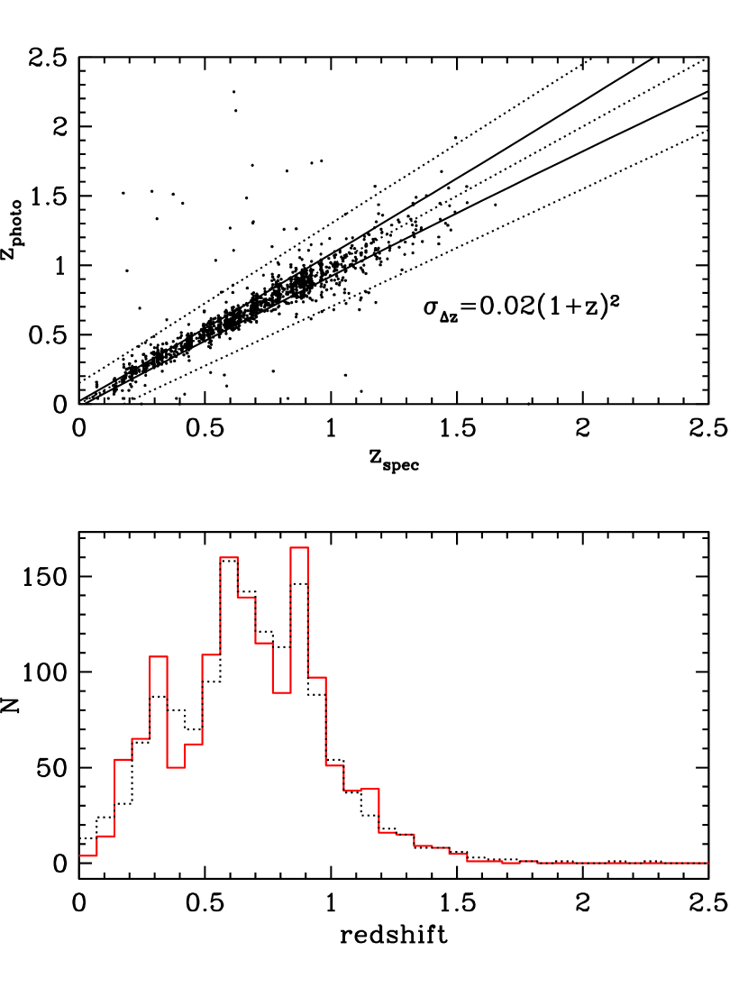
Figure 1: Upper panel: Comparison of photometric and spectroscopic redshifts in the $K$-selected sample for objects with highly reliable (confidence level $>97\%$ , i.e. about 1400 galaxies with flag=3, 4) spectroscopic redshifts. The accuracy obtained is $\sigma_{\Delta z}=0.02(1+z)^{2}$ (shown as solid lines) with only 3.7% of outliers, defined as the objects outside the region limited by the 2 dotted lines ($z_{photo}=z_{spec}\pm 0.15(1+z_{spec})$) in the figure. Lower panel: Spectroscopic (solid line) and photometric (dotted line) redshift distribution for the same comparison sample.

2.1 The $I$-selected Spectroscopic Sample

In this study we use the F02-VVDS deep spectroscopic sample, purely magnitude limited ($17.5\leq I\leq 24$), in combination with the multi-wavelength optical/near-IR dataset. From the total sample of $8281$ objects with measured redshift, we removed the spectroscopically confirmed stars and broad line AGN, as well the galaxies with low quality redshift flag (i.e. flag 1), remaining with 6419 galaxy spectra with secure spectroscopic measurement (flags 2, 3, 4, 9), corresponding to a confidence level higher than 80%. Galaxies with redshift flags 0 and 1 are taken into account statistically (see Section 4 and Ilbert et al. 2005 and Zucca et al. 2006 for details). This spectroscopic sample has a median redshift of $\sim 0.76$. Compared to previous optically selected samples, the VVDS has not only the advantage of having an unprecedented high fraction of spectroscopic redshifts (compared, for example, to the purely photometric redshifts as in COMBO17, Wolf et al. 2003 and Borch et al. 2006 for the MF), but also of being purely magnitude selected ($17.5<I<24$), differently, for example, from the DEEP2 (Bundy et al. bun06 (2006) for the MF) survey, which has a colour-colour selection. Moreover, the VVDS covers an area from 10 to 40 times wider than the GOODS-MUSIC field (Fontana et al. 2006) and the FORS Deep Field (FDF, Drory et al. 2005), respectively.

2.2 The $K$-selected Photometric Sample

A wide part of the VVDS-02h field (about 623 arcmin²) has been observed also in the near-IR (Iovino et al. 2005, Temporin et al. in preparation). This allows us to build a $K$-selected sample with a total area of 610 arcmin² (after excluding low-S/N borders): 442 arcmin² are 90% complete to $K<22.34$, while 168 arcmin² are 90% complete to $K<22.84$ (equivalent to $K_{\rm Vega}=21$).

This sample consists of $11221$ objects, of which $2882$ have VVDS spectroscopy. In particular, the deep sample ($K<22.84$) consists of $3821$ objects, of which 749 have VVDS spectroscopy, and 596 of them are galaxies with a secure spectroscopic identification (flags 2, 3, 4, 9). This latter deep sample is more than one magnitude deeper than the samples from the K20 spectroscopic survey (Cimatti et al. 2002) and the MUNICS survey (Drory et al. 2001). Additionally, the total $K$-selected sample covers an area more than 10 times wider than the K20 and the GOODS-CDFS sample used by Drory et al. (2005) and 4 times wider than the GOODS-MUSIC field (Fontana et al. 2006).

Since the spectroscopic sampling of the $K$-selected sample is less than satisfactory, we take advantage of the high quality photometric redshifts ($z_{photo}$). The method and the calibration are presented and discussed in Ilbert et al. (2006). The comparison sample contains 3241 accurate spectroscopic redshifts (confidence level $>97\%$ , i.e. flag=3, 4) up to $I=24$ obtaining a global accuracy of $\sigma_{\Delta z/(1+z)}=0.037$ with only 3.7% of outliers. Also in the $K$-selected photometric sample the agreement between photometric and highly reliable spectroscopic redshifts (about 1400) is excellent (Figure 1). We note, however, a non-negligible number of catastrophic solutions with $z_{photo}\lower 2.15277pt\hbox{$\;\buildrel>\over{\sim}\;$}1.2$ and $z_{spec}\lower 2.15277pt\hbox{$\;\buildrel<\over{\sim}\;$}1$ which could introduce a bias at high-redshift (see also discussion in Section 2.3). Even if we cannot rely on a wide spectroscopic comparison sample at high-$z$, the number of galaxies with $z_{photo}>1.2$ is similar or only slightly higher (about 20%) than the number of galaxies with $z_{spec}>1.2$ (63 vs. 51, see Figure 1) and have very similar fluxes and colors. For this reason we do not expect that our results on the mass function and the mass density will be strongly biased by the effect of catastrophic redshifts (see Section 4). Furthermore, at high-$z$ the dispersion between photometric and spectroscopic redshifts increases, but not drammatically, to $\sigma_{\Delta z/(1+z)}\simeq 0.05,0.06$ at $z>1.2,1.4$. Over the whole redshift range it can be represented with $\sigma_{\Delta z}\simeq 0.02(1+z)^{2}$ (shown in Figure 1).

For the whole $K$-selected sample, the median errors on photometric redshifts, based on $\chi^{2}$ statistics, are $\sigma_{zphoto}=0.06$ (0.04 at $z<1$, increasing to 0.14 at $z>1.5$). As expected, there is also an increase of $\sigma_{zphoto}$ for the faintest objects, but this increase is only about 0.02 in the faintest magnitude bin. As previously noted by Ilbert et al. (2006) the statistical errors are consistent with $\sigma_{\Delta z}$ and could be used as an indication of their accuracy. We will discuss in the following sections the effects of these uncertainties and conclude that they do not affect significantly our conclusions.

We note, moreover, that the $K$-selected sample selects a different population, in particular of Extremely Red Objects (EROs) at $z_{photo}>1$ (see Section 2.3 and Fig. 3), compared to the $I$-selected sample used to calibrate the derived photometric redshift. Actually, photometric redshifts greater than 0.8-1.0 for the EROs population have been confirmed spectroscopically with very low contamination of low-$z$ objects (Cimatti et al. 2002). Moreover, the near-IR bands are crucial to constrain photometric redshifts in the redshift desert since the $J$-band is sensitive to the Balmer break up to $z=2.5$. Indeed Ilbert et al. (2006) obtain for the deep sample at $K<23$ the most reliable photometric redshifts on this sub-sample with only 2.1% of outliers and $\sigma_{\Delta z/(1+z)}=0.035$ (see their figure 13).

In this paper we therefore use photometric redshifts for the whole $K$-selected photometric sample and the highly reliable spectroscopic redshifts when available.

In order to select galaxies from the total $K$-selected photometric sample, we have used a number of photometric methods to remove candidate stars, as described below. Some of the possible criteria to select stars are: (i) the CLASS_STAR parameter given by SExtractor (Bertin & Arnouts ber96 (1996)), providing the “stellarity-index” for each object, reliable up to $I\simeq 21$; (ii) the FLUX_RADIUS_K parameter, computed by SExtractor from the $K$ band images, which gives an estimate of the radius containing half of the flux for each object; this can be considered a good criterion to isolate point-like sources up to $K\simeq 19$ (see Iovino et al. 2005); (iii) the $BzK$ criterion, proposed by Daddi et al. (2004a), with stars characterized by colours $z-K<0.3(B-z)-0.5$; (iv) the $\chi^{2}$ of the SED fitting carried out during the photometric redshift estimate (Ilbert et al. 2006), with template SEDs of both stars and galaxies.

To efficiently remove stars in the whole magnitude range of our sample, avoiding as much as possible to lose galaxies, we decided to use the intersection of the first three criteria. We therefore selected as stars the objects fulfilling all the constraints (i) CLASS_STAR $\geq 0.95$ for $I<22.5$ or CLASS_STAR $\geq 0.90$ if $I>22.5$, (ii) FLUX_RADIUS_K $<3.4$ and (iii) $z-K<0.3(B-z)-0.5$. When it was not possible to apply criterion (iii), because of non detection either in the $B$ or $z$ filters, we used criterion (iv) in its place. Furthermore, we added to the sample of candidate stars also the objects with $K<16$ and FLUX_RADIUS_K $<4$, to be sure to exclude from the galaxy sample these saturated point-like objects. The final sample consists of 653 candidate stars, which we have removed from the sample in the following analysis. Comparing to the spectroscopic subsample (we remind that stars were not excluded from the spectroscopic targets of VVDS), we found about 87% of efficiency to photometrically select stars, i.e. only 28 out of the 214 spectroscopic stars have not been selected in this way, and only 3 (1.4%) with highly reliable spectroscopic flag (3, 4), whereas 21 spectroscopic extragalactic objects (less than 1%) fall inside the candidate star sample. Three of them are broad line AGN and the others are all compact objects, most of them with redshift flags 1 or 2 and only one with flag 3. This latter object has not been eliminated from the galaxy sample. We have furthermore removed from the galaxy sample the spectroscopically confirmed AGNs and the three secure spectroscopic stars which were not removed with the photometric criteria.

The final $K$-selected sample consists of $10160$ galaxies with either photometric redshifts or highly reliable spectroscopic redshifts, when available, in the range between $0$ and $2.5$: $6720$ galaxies in the shallow $K<22.34$ area of $442$ arcmin² and $3440$ galaxies in the deeper area ($K<22.84$) of $168$ arcmin².

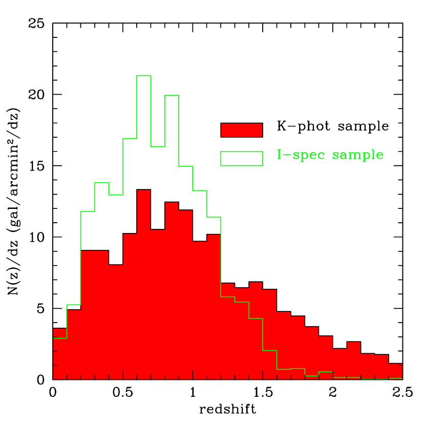
Figure 2: Redshift distributions for the $K$-selected photometric sample (filled histogram) and for the $I$-selected spectroscopic sample (empty histogram).

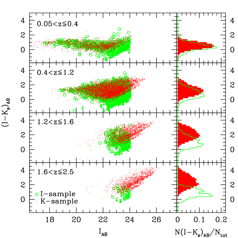
Figure 3: Colour-magnitude diagram and colour distribution at different redshifts for the $K$-selected photometric sample (filled squares and histogram) and for the $I$-selected spectroscopic sample (open circles and empty histogram)

2.3 Comparison of the Two Samples

As shown in Fig. 2, the redshift distribution in the $K$-selected sample peaks at higher redshift than in the $I$-selected spectroscopic sample, with the two median redshifts being 0.91 and 0.76, respectively. Even if we cannot rely on a wide spectroscopic comparison sample at high-$z$, we have better investigated the reliability of the high-$z$ tail in the $K$-selected sample in term of fraction and colors. We found indeed that at $K<22$ the fraction of objects with $z>1,1.5$ ($35,13$% respectively) is similar to previous spectroscopic (K20 survey, see Cimatti et al. 2002) or photometric studies (Somerville et al. 2004). Moreover, we have used the $BzK$ color-color diagnostic proposed and calibrated on a spectroscopic sample to cull galaxies at $1.4<z<2.5$ (Daddi et al. 2004). We found that most (92%) of the galaxies at $1.5<z_{photo}<2.5$ lie in the high-$z$ region of the $BzK$ diagram.

We conclude that our $K$-selected sample shows no indication of significant bias in its high-redshift tail. The global $(I-K)$ colour distributions of the two samples are similar to each other up to $z\sim 1.2$ (see right panels in Fig. 3), but they are significantly different at higher redshift. At $z>1.2$ the $I$-selected sample misses many red galaxies fainter than the $I$ limit, most of them being Extremely Red Objects (EROs: defined as objects with colours $I-K>2.6$), which are instead included in the $K$ sample ($\sim 81$% of EROs in the deep $K<22.84$ sample have $I>24$). For this reason the $K$-selected sample is more adequate to study the massive tail of the GSMF at high-$z$. Vice versa, the $K$-selected sample misses at all redshifts a number of faint blue galaxies, which are included in the $I$-selected spectroscopic sample (see left panels in Fig. 3). These faint blue galaxies are important in the estimate of the low-mass tail of the GSMF.

3 Estimate of the Stellar Masses

The rest-frame near-IR light has been widely used as a tracer of the galaxy stellar mass, in particular for local galaxies (e.g. Gavazzi et al. 1996; Madau, Pozzetti & Dickinson 1998, Bell & de Jong 2001). However, an accurate estimate of the galaxy stellar mass at high $z$, where galaxies are observed at widely different evolutionary stages, is more uncertain because of the variation of the ${\cal M}_{\rm stars}/L_{K}$ ratio as a function of age and other parameters of the stellar population, such as the star formation history and the metallicity. The use of multiband imaging from UV to near-IR bands is a way to take into account the contribution to the observed light of both the old and the young stellar populations in order to obtain a more reliable estimate of the stellar mass.

However, even stellar masses estimated using the fit to the multicolour spectral energy distribution (SED) are model dependent (e.g. changing with different assumptions on the initial mass function, IMF) and subject to various degeneracies (age – metallicity – extinction). In order to reduce such degeneracies we have used a large grid of stellar population synthesis models, covering a wide range of parameters, in particular in star formation histories (SFH). Indeed, in the case of real galaxies the possibly complex star-formation histories and the presence of major and/or minor bursts of star formation can affect the derived mass estimate (see Fontana et al. 2004).

We have applied and compared two different methods to estimate the stellar masses from the observed magnitudes (using 12 photometric bands from $u^{*}$ to $K$), that are based on different assumptions on the star-formation history. For both of them we have adopted the Bruzual & Charlot (2003; BC03 hereafter) code for spectral synthesis models, in its more recent rendition, using its low resolution version with the “Padova 1994” tracks. Different models have also been considered, e.g. Maraston 2005, and Pégase models (Fioc and Rocca-Volmerange 1997). The results obtained with these models are compared with those obtained with the BC03 models at the end of Section 3.1.

Since most of previous studies at high-$z$ assumed models with exponentially decreasing SFHs, we have used the same simple smooth SFHs (see Section 3.1) in order to compare our results with those of previous surveys. In addition, to further test the uncertainties in mass determination, we have used models with complex SFHs (see Section 3.2), in which secondary bursts have been added to exponentially decreasing SFHs. These models have been widely used in studies of SDSS galaxies (see Kauffmann et al. 2003 and Salim et al. 2005 for further details). Table 1 summarizes the model parameters used in the 2 methods described in the following sections.

In our analysis we have adopted the Chabrier IMF (Chabrier et al. 2003), with lower and upper cutoffs of 0.1 and 100 $M_{\odot}$. Indeed, all empirical determinations of the IMF indicate that its slope flattens below $\sim 0.5\;M_{\odot}$ (Kroupa kro01 (2001), Gould et al. gou96 (1996), Zoccali et al. zoc00 (2000)) and a similar flattening is required to reproduce the observed ${\cal M}_{\rm stars}/L_{B}$ ratio in local elliptical galaxies (see e.g. Renzini ren05 (2005)). As discussed extensively by Bell et al. (2003), the Salpeter IMF (Salpeter 1955) is too rich in low mass stars to satisfy dynamical constraints (Kauffmann et al. 2003, Kranz et al. 2003). Moreover, di Serego Alighieri et al. (2005) show a rather good agreement between dynamical masses and stellar masses estimated with the Chabrier IMF at $z\sim 1$. Specifically, this is true at least for high-mass elliptical galaxies, less affected than lower-mass galaxies by uncertainties in the estimate of their dynamical mass due to possibly substantial rotational contribution to the observed velocity dispersion.

At fixed age the masses obtained with the Chabrier IMF are smaller by a factor $\sim 1.7$, roughly independent of the age of the population, than those derived with the classical Salpeter IMF, used in several previous works that we shall compare with (e.g. Brinchmann & Ellis 2000; Cole et al. 2001; Dickinson et al. 2003; Fontana et al. 2004). We have checked this statement in our sample, finding a systematic median offset of a factor $1.7$ and a very small dispersion ($\sigma=0.082$ dex) in the masses derived with the two different IMFs. Since this ratio is approximately constant for a wide range of star formation histories (SFH), the uncertainty in the IMF does not introduce a fundamental limitation with respect to the results we will discuss in the following Sections. Even if the absolute value of the mass estimate is uncertain, the use of Salpeter or Chabrier IMFs does not introduce any significant difference in the relative evolution with redshift of the mass function and mass density.

One possible limitation of our approach to derive stellar masses in our sample is the contamination by narrow-line AGN (broad line AGN have been already excluded, see Section 2.1). From the available spectroscopic diagnostic, in the $I$-selected spectroscopic sample at the mean redshift $z\simeq 0.7$, we found that the contamination due to type II AGN is less than 10%. Recently, several studies (Papovich et al. 2006, Kriek et al. 2007, Daddi et al. 2007) suggest that the fraction of type II AGN increases with redshift and stellar mass. According to Kriek et al. (2007) at $2<z<2.7$ and $K<21.5$ the fraction is about $20\%$ for massive ($2.9\times 10^{11}M_{\odot}$ for a Salpeter IMF) galaxies. To derive the contribution of type II AGN to the massive tail of the MF is beyond the scope of this paper. However we note, as shown also by the above studies, that for most of these objects the optical light is dominated by the integrated stellar emission. Therefore, both our photometric redshift and mass estimates are likely to be approximately correct also for them.

3.1 Smooth SFHs

Consistently with previous studies, we have used synthetic models with smooth SFH models (exponentially decreasing SFH with time scale $\tau$: $SFR(t)\propto\exp(-t/\tau)$) and a best-fit technique to derive stellar masses from multicolour photometry.

To this purpose we have developed the code HyperZmass, a modified version of the public photometric redshift code HyperZ (Bolzonella et al. 2000): like the public version, HyperZmass uses the SED fitting technique, computing the best fit SED by minimizing the $\chi^{2}$ between observed and model fluxes. We used models built with the Bruzual & Charlot (2003) synthetic library. When the redshift is known, either spectroscopic or photometric, the best fit SED and its normalization provide an estimate of the stellar mass contained in the observed galaxy. In particular, we estimate the stellar mass content of the galaxies, derived by BC03 code, by integrating the star formation history over the galaxy age and subtracting from it the “Return fraction” (R) due to mass loss during the stellar evolution. For a Chabrier IMF, this fraction is already as high as $\sim 40$% at an age of the order of 1 Gyr and approaches asymptotically about 50% at older ages.

The parameters used to define the library of synthetic models are listed in Table 1. Similar parameters have been used in Fontana et al. (2004). The Calzetti (2000) extinction law has been used. Following that paper, we have excluded from the grid some models which may be not physical (e.g. those implying large dust extinctions, $A_{V}>0.6$, in absence of a significant star-formation rate, $Age/\tau>4$, see Table 1). To better match the ages of early-type galaxies in the local universe and following SDSS studies, we also removed models with $\tau<1$ Gyr and with star formation starting at $z<1$.

We find that the “formal” typical $1\sigma$ statistical errors (defined as the 68% range as derived from the $\chi^{2}$ statistics) on the estimated masses, not taking into account the error on the estimate of the photometric redshift for the $K$-selected sample, are of the order of $0.04$ dex for the $K$-selected sample and 0.05 for the $I$-selected sample. A more reliable estimate of the errors has been obtained using HyperZ to simulate catalogs to the same depth of our sample (see Bolzonella et al. 2000). Using all 12 photometric bands (from $u^{*}$ to $K$), available for a subset of our data, and realistic photometric errors, the recovered stellar masses reproduce the input masses with no significant offset and a dispersion of 0.12 dex up to $z\sim 3$. For comparison, using only the optical bands (from $u^{*}$ to $z^{\prime}$) the dispersion increases to $\sim 0.49$ dex at $z>1$. The best fit masses obtained from input simulations built using randomly all available metallicities and analyzed only with solar metallicity models are not significantly shifted from the input masses, but the dispersion increases from 0.12 dex to 0.21 dex. These dispersions, computed using a $4\sigma$ clipping, provide an estimate of the minimum, intrinsic uncertainties of this method at our depth. For the $K$-selected photometric sample further uncertainties in the fitting technique are due to the photometric redshift accuracy ($\sigma_{\Delta z}\simeq 0.02(1+z)^{2}$ up to $z=2.5$) which corresponds on average to about 0.12 dex of uncertainty in mass, being larger at low redshift ($\sim$ 0.2 dex at $z<0.4$) than at high-$z$ ($\sim 0.10$ dex at $z=2$).

Although in principle the best-fitting technique provides estimates also for age, metallicity, dust content and SFH timescale, our simulations show that on average all these quantities are much more affected by degeneracies and therefore less constrained than the stellar mass.

Table 1: Parameters Used for the Library of Template SEDs

$$\begin{array}[]{p{0.3\linewidth}ll}\hline\cr\hline\cr\vskip 3.0pt plus 1.0pt minus 1.0pt\cr Method&Smooth\leavevmode\nobreak\ SFHs&Complex\leavevmode\nobreak\ SFHs\\ \vskip 3.0pt plus 1.0pt minus 1.0pt\cr\hline\cr\hline\cr\vskip 3.0pt plus 1.0pt minus 1.0pt\cr IMF&Chabrier&Chabrier\\ \vskip 3.0pt plus 1.0pt minus 1.0pt\cr\hline\cr\vskip 3.0pt plus 1.0pt minus 1.0pt\cr SFR $\tau$ (Gyr)&[0.1,\infty]^{\mathrm{a}}&[1,\infty]\\ \vskip 3.0pt plus 1.0pt minus 1.0pt\cr\hline\cr\vskip 3.0pt plus 1.0pt minus 1.0pt\cr log(Age)${}^{\mathrm{b}}$ (yr)&[8,10.2]&[8,10]\\ \vskip 3.0pt plus 1.0pt minus 1.0pt\cr\hline\cr\vskip 3.0pt plus 1.0pt minus 1.0pt\cr burst age (yr)&-&[0,10^{10}]\\ \vskip 3.0pt plus 1.0pt minus 1.0pt\cr\hline\cr\vskip 3.0pt plus 1.0pt minus 1.0pt\cr burst fraction&-&[0,0.9]\\ \vskip 3.0pt plus 1.0pt minus 1.0pt\cr\hline\cr\vskip 3.0pt plus 1.0pt minus 1.0pt\cr Metallicities&Z_{\odot}&[0.1Z_{\odot},2Z_{\odot}]\\ \vskip 3.0pt plus 1.0pt minus 1.0pt\cr\hline\cr\vskip 3.0pt plus 1.0pt minus 1.0pt\cr Extinction&Calzetti\leavevmode\nobreak\ law&Charlot\&Fall\leavevmode\nobreak\ model\\ &&(n=0.7,\mu\in[0.1,1])\\ \vskip 3.0pt plus 1.0pt minus 1.0pt\cr\hline\cr\vskip 3.0pt plus 1.0pt minus 1.0pt\cr Dust content&A_{V}^{\mathrm{c}}\in[0,2.4]&\tau_{V}\in[0,6]\\ \vskip 3.0pt plus 1.0pt minus 1.0pt\cr\hline\cr\end{array}$$

• $\tau<1$ if star formation starts at $z<1$.

• At each redshift, galaxies are forced to have ages smaller than the Hubble time at that redshift.

• $A_{V}<0.6$ if $Age/\tau>4$.

In addition, we have compared our derived masses with those obtained by using different population synthesis models, such as Pégase and Maraston (2005) models. In particular, Maraston (2005) models include the thermally pulsing asymptotic giant branch (TP-AGB) phase, calibrated with local stellar populations. This stellar phase is the dominant source of bolometric and near-IR energy for a simple stellar population in the age range 0.2 to 2 Gyr. We have tested the differences with BC03 models using the $I$-selected spectroscopic sample and we found only a small but systematic shift ($\sim-0.14$ dex and a similar dispersion) up to $z\sim 1.2$ both with and without the use of near-IR photometry. On the contrary, masses derived using Pégase models and similar SFHs have instead no significant offset.

At higher redshifts the differences between our estimated masses and those obtained with Maraston models in the $K$-selected spectroscopic subsample are slightly smaller and even smaller in the $K$-selected photometric sample ($\sim-0.11,-0.08$, respectively). This differences are smaller than that found by Maraston et al. (2006), $\sim-0.2$, in their SED fitting (from $B$ up to Spitzer IRAC and MIPS bands) of a few high redshift passive galaxies with typical ages in the range 0.5 – 2.0 Gyr, selected in the Hubble Ultra Deep Field (HUDF). This difference between our results and those of Maraston et al. could be due to a combination of effects, such as the absence in our photometric data of mid-IR Spitzer photometry, which at these redshifts is sampling the rest frame near-IR part of the SED, mostly influenced by the TP-AGB phase, and also to the wide range of complex stellar populations in our sample, in which the effect of the TP-AGB phase may be diluted by the SFH.

3.2 Complex SFHs

Real galaxies could have undergone a more complex SFH, in particular with the possible presence of bursts of star formation on the top of a smooth SFH. Thus, we have computed masses also following a different approach, which has been intensively used in previous studies of SDSS galaxies (e.g. Kauffmann et al. 2003, Brinchmann et al. 2004, Salim et al. 2005, Gallazzi et al. 2005). In this approach we parameterize each SF history in terms of two components: an underlying continuous model, with an exponentially declining SF law ($SFR(t)\propto\exp(-t/\tau)$), and random bursts superimposed on it. We assume that random bursts occur with equal probability at all times up to galaxy age. They are parameterized in terms of the ratio between the mass of stars formed in the burst and the total mass of stars formed by the continuous model over the age. This ratio is taken to be distributed between 0.0 and 0.9. During a burst, stars are assumed to form at a constant rate for a time distributed uniformly in the range 30 – 300 Myr. The burst probability is set so that 50% of the galaxies in the library have experienced a burst in the past 2 Gyr. Attenuation by dust is described by a two-component model (see Charlot & Fall 2000), defined by two parameters: the effective $V$-band absorption optical depth $\tau_{V}$ affecting stars younger than 10 Myr and arising from giant molecular clouds and the diffuse ISM, and the fraction $\mu$ of it contributed by the diffuse ISM, that also affects older stars. We take $\tau_{V}$ to be distributed between 0 and 6 with a broad peak around 1 and $\mu$ to be distributed between 0.1 and 1 with a broad peak around 0.3. Finally, our model galaxies have metallicities uniformly distributed between 0.1 and 2 $Z_{\odot}$.

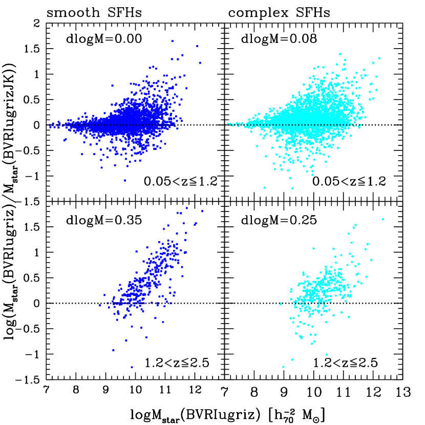
Figure 4: Effect of NIR photometry in the mass determination: ratio between masses estimated without and with NIR photometry vs. mass determined without NIR photometry. The data have been splitted into different redshift ranges. Left: masses determined using smooth SFHs. Right: The same, but using complex SFHs

The model spectra are computed at the galaxy redshift and in each of them we measure the $k$-shifted model magnitudes for each VVDS photometric band. We also force the age of all models in a specific redshift range to be smaller than the Hubble time at that redshift. The model SEDs are then scaled to each observed SED with a least squares method and the same scaling factor is applied to the model stellar mass. We compare the observed to the model fluxes in each photometric band and the $\chi^{2}$ goodness of fit of each model determines the weight ($\propto\exp[-\chi^{2}/2]$) to be assigned to the physical parameters of that model when building the probability distributions for each parameter of any given galaxy. The probability distribution function (PDF) of a given physical parameter is thus obtained from the distribution of the weights of all models in the library at the specified redshift. We characterize the PDF using its median and the 16 – 84 percentile range (equivalent to $\pm 1\sigma$ range for Gaussian distributions), and also record the $\chi^{2}$ of the best-fitting model.

Similarly to what has been done for the models with smooth SFH (see Section 3.1), also in this case the stellar mass content of galaxies is derived by subtracting the return fraction R from the total formed stellar mass. We find that the average “formal” $1\sigma$ error (defined as half of the 16 – 84 percentile range) on the estimated masses is of the order of $0.09$ dex for the $K$-selected sample. The average error increases with redshift from $\sim 0.06$ dex at low redshift to $\sim 0.11$ dex at $1<z<2$ and decreases with increasing mass from $\sim 0.08$ dex for $\log M<10$ to $\sim 0.05$ for $\log M>10$ at $z\simeq 0.7$. In the $K$-selected sample the photometric redshift accuracy induced a further uncertainty on the mass of the order of 30% up to $z>1.5$. In the $I$-selected sample, where near-IR photometry is not always available, the typical error on the mass is larger and is of the order of $\sim 0.13$ dex.

3.3 Effect of NIR Photometry

For about half of the sources in the $I$-selected sample only optical photometry is available. We have therefore used the results obtained for the $K$-selected spectroscopic subsample to better understand the reliability of the mass estimates in the whole $I$-selected sample and quantify potential systematic effects. We found that the mass estimates derived using only optical bands are on average in rather good agreement with those obtained using also NIR bands up to $z\sim 1.2$. In absence of NIR bands the galaxy stellar masses tend to be only slightly overestimated, with a median shift $<0.1$ dex; this is due to the fact that already at $z=0.4$, for example, the $z^{\prime}$-band (the reddest band used in the fit in absence of NIR) samples the $R$-band rest-frame and therefore the SED fitting is less reliable for the estimate of the stellar masses. There is however a significant fraction of the galaxies for which the ratio between the two masses is higher than a factor of three (see upper panels of Fig.4). This fraction of galaxies with significantly discrepant mass estimates is $\sim$ 5% for the models with smooth SFH and $\sim 9$ % for the models with complex SFH.

At higher redshifts, where our reddest optical band, i.e. the $z$-band, is sampling the rest-frame spectrum bluewards of the 4000 Å break, the comparison of the two sets of mass estimates (i.e. with and without near-IR photometry) is significantly worse. Not only the median shift increases significantly, but also the ratio of the two sets of masses is significantly correlated with the mass derived without using NIR photometry (see lower panels of Fig. 4). For this reason, we have decided to use the whole $I$-selected VVDS spectroscopic sample only up to $z\sim 1.2$, whereas at higher redshifts we use as reference the $K$-selected photometric sample.

As shown in the upper panels of Fig.4, the ratio between the masses computed without and with NIR photometry has a non-negligible dispersion also for $z<1.2$, with the masses computed without NIR photometry being higher on average. In order to statistically correct for this effect, we have performed the following Monte Carlo simulation. For each galaxy without near-IR photometry in the $I$-selected spectroscopic sample we have applied a correction factor to its estimated mass. This correction factor has been derived randomly from the observed distribution, at the mass of each galaxy, of the ratios of the masses with and without NIR photometry. The effect on the mass function of using these “statistically corrected” masses is shown and discussed in Sect. 4.

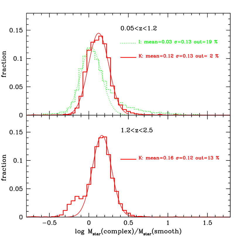
Figure 5: Histograms of the ratio of the masses derived with the smooth and the complex star formation histories. In the upper panel ($z<1.2$) both data from the $I$-selected and the $K$-selected samples are shown; in the lower panel ($z>1.2$) only data from the $K$-selected sample are shown, since the $I$-selected sample is not used to derive the mass function in this redshift range.

3.4 Comparison of the Masses Obtained with the Two Methods

In this section we compare the mass estimates we obtained using the two different methods described above for the VVDS galaxies. Since the ratio of the two estimates is almost independent of the mass, in Fig. 5 we show the histograms of this ratio, integrated over all masses, for two different redshift bins. In the upper panel ($z<1.2$), both data from the $I$-selected and the $K$-selected samples are shown; in the lower panel only data from the $K$-selected sample are shown, since the $I$-selected sample is not used to derive the mass function in this redshift range. Gaussian curves, representing the bulk of the population, are drawn on the top of each histogram. The parameters of each Gaussian are reported in the figure.

The global comparison of the two sets of masses is rather satisfactory, even if it shows a systematic shift, larger for the $K$-selected sample, between the two sets of masses, with the ‘smooth SFH’ masses being on average smaller than the ‘complex SFH’ masses. The values of $\sigma$ of these Gaussians are similar, of the order of $0.13$ dex. However, in two of the three cases (i.e. the $I$-selected sample at low redshift and the $K$-selected sample at high redshift) the distributions of the ratio of the masses appear to be asymmetric, with tails which are not well represented by a Gaussian distribution. The fractions of these “outliers” are given in Fig. 5. This tail is particularly significant for the $I$-selected sample, for which there are galaxies with the ratio between the two masses higher than 3 and in a few cases reaching a value of 10.

We have analyzed the effect of the different parameters used in the two methods. The impact of different extinction curves on the mass estimates has already been investigated by Papovich et al. (2001), Dickinson et al. (2003), Fontana et al. (2004), and found to be small. We have repeated the same exercise for the two different dust attenuation models adopted, finding that for a given SFH the mass estimated with different extinction laws are similar, with an average shift of 0.02 dex.

Analyzing in some detail the properties of the galaxies which are in the extended tail of large mass ratios for the $I$-selected sample at low redshift (see the upper panel in Fig. 5), we found that, even if many of them do not have near-IR photometry and therefore their mass is more uncertain (see previous section), on average they are characterized by blue colours in the bluer bands ($B-I$) and red colours in the redder bands ($I-z$ or $I-K$). Because of this, they have been fitted typically with low values of the population age by HyperZmass with a smooth SFH, while the estimate obtained with a complex SFH corresponds to an older, and therefore more massive, population plus a more recent burst with a mass fraction in the burst of the order of ${\it fburst}<0.15$. Vice versa the low ratio outliers in the $K$-selected sample at high redshift have been fitted typically with moderately higher dust content by HyperZmass than with complex SFHs. Finally, we conclude that the main differences between the two methods to determine the masses are largely due to different assumed SFHs and, in particular, to the secondary burst component allowed in the model with complex SFHs.

To summarize, we have explored in detail two different methods and a wide parameter space (see Table 1) to estimate the stellar mass content in galaxies in order to better understand the uncertainties in the photometric stellar mass determinations. Indeed, a good estimate of the intrinsic errors may be critical for the GSMF measurement and interpretation. We found that, within a given assumption on the SFH, the accuracy of the photometric stellar mass is overall satisfactory, with intrinsic uncertainties in the fitting technique of the order of $\sim$ 30%, in agreement with similar results in the K20 (Fontana et al. 2004), HDFN (Dickinson et al. 2003) and HDFS (Fontana et al. 2003) at the same redshifts. These errors are smaller than the estimates at higher redshift ($z\simeq 3$) (Papovich et al. (2001), Shapley et al. (2001)), since at our average redshifts ($z\simeq 0.7-1$) we can rely on a better sampling of the rest-frame near-IR part of the spectrum, while are similar to the uncertainties estimated at high-$z$ using IRAC data by Shapley et al. (2005). For the $K$-selected photometric sample the uncertainties in the stellar mass due to the photometric redshift errors are on average of the order of 30% up to $z>1.5$, giving a total fitting uncertainty up to 45% at $z>1.5$. Finally, systematic shifts, mainly due to different assumptions on the SFHs, can be as large as $\sim$ 40% over the entire redshift range $0.05<z<2.5$ when NIR photometry is available. The uncertainty in the derived masses is obviously higher also at low redshift when NIR photometry is not available and in this case it becomes extremely large at $z>1.2$ (see Fig.4).

For what concerns the absolute value of the mass, its uncertainty is mainly due to the assumptions on the IMF and it is within a factor of 2 for the typical IMFs usually adopted in the literature.

In the following sections we discuss in some detail the effects of the two methods on the derivation of the GSMF.

3.5 Massive Galaxies at $z>1$

Figure 6 shows the stellar masses for the 2 samples ($I$ and $K$-selected) derived using the smooth SFHs. It is interesting to note the presence of numerous massive objects ($\log M>11$) at all redshifts and up to $z=2.5$. High-$z$ massive galaxies have been already observed in previous surveys (Fontana et al. 2004, Saracco et al. 2005, Cimatti et al. 2004, Glazebrook et al 2004, Fontana et al. 2006, Trujillo et al. 2006). Here the relatively wide area (the $K$-selected sample is more than 10 times wider and from 0.5 to 1 magnitude deeper than the K20 survey) allows to better sample the massive tail of the population. We note that massive galaxies have typically redder optical-NIR rest-frame colours ($\langle M_{I}-M_{K}\rangle\simeq 0.7$) compared to the whole population ($\langle M_{I}-M_{K}\rangle\simeq 0.5$), consistently with the idea that massive galaxies host the oldest stellar population. Further analysis of the stellar population properties and spectral features of massive galaxies, as well as of red objects will be presented in forthcoming papers (Lamareille et al. in preparation, Vergani et al. 2007, Temporin et al. in preparation).

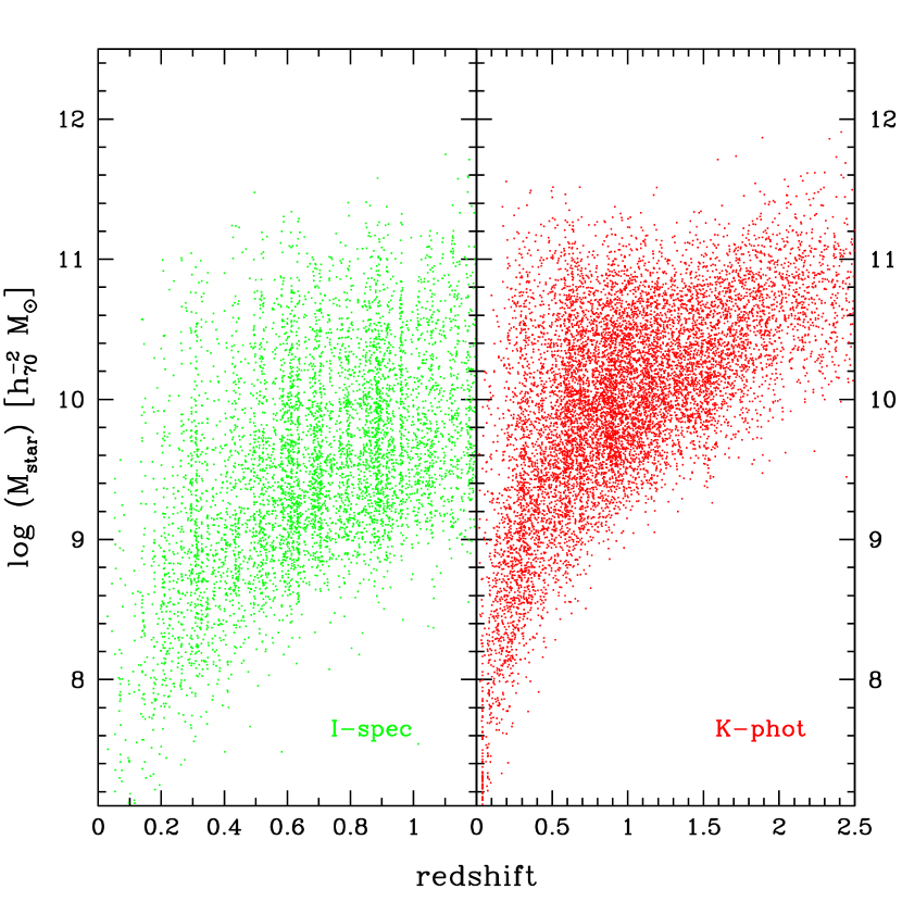
Figure 6: Stellar Mass as a function of redshift for the $I$-selected spectroscopic (left) and for the $K$-selected photometric (right) samples for smooth SFHs.

Figure 7: Effect on the $I$-selected MF of the use of the statistically corrected masses, which take into account the effect of near-IR photometry on the mass determination (see text for details). Complex SFHs have been used to derive masses. Empty circles represent the MF obtained using the original uncorrected masses, filled squares show the MF obtained using the statistically corrected masses. For comparison the STY Schechter MF is shown for the subsample where near-IR photometry is available. The vertical dashed lines represent the completeness limit of the sample as defined in the text.

Figure 8: $K$-selected MF derived from the 2 subsamples, deep (filled circles) and shallow (empty circles), separately (smooth SFHs have been used to derive masses). For comparison the STY Schechter MF for the global $K$-selected sample is shown. The vertical dashed lines represent the completeness limit of the 2 $K$-selected subsamples.

4 Mass Function Estimate

Once the stellar mass has been estimated for each galaxy in the sample, the derivation of the corresponding Galaxy Stellar Mass Function (MF) follows the traditional techniques used for the computation of the luminosity function. Here we apply both the classical non-parametric $1/V_{\rm max}$ formalism (Schmidt 1968, Felten 1976) and the parametric STY (Sandage, Tammann & Yahil 1979) method to estimate best-fit Schechter (1976) parameters ($\alpha,{\cal M}_{\rm stars}^{*},\phi^{*}$). In the case of the $K$-selected sample, in order to take into account the two different magnitude limits, we perform a “Coherent Analysis of independent samples” as described by Avni & Bahcall (1980).

Ilbert et al. (ilbert04 (2004)) have shown that the estimate of the faint end of the global luminosity function can be biased, because, due to different k-corrections, different galaxy types have different absolute magnitude limits for the same apparent magnitude limit. The same bias is present also for the low mass end of the mass function. This is due to the fact that, because of the existing dispersion in the mass-to-light ratio of different galaxy types, at small masses the objects with the largest mass-to-light ratio are not included in a magnitude limited sample (see Appendix B in Fontana et al. 2004 for an extensive discussion). For this reason, when computing the global mass functions with the STY method, in order to fully avoid this bias, we should use in each redshift range only galaxies above the stellar mass limit where all the SEDs are potentially observable. In both the $K$- and $I$-selected samples these limits derive from the conversion between photometry and stellar mass for early-type galaxies and are very restrictive. However, recent results show that the faint-end and the low-mass end of the luminosity and mass function is dominated by late-type galaxies up to $z\sim 2$ (Fontana et al. 2004, Zucca et al. 2006, Bundy et al. 2006). Therefore for the STY estimate we will use as lower limit of the mass range the minimum mass above which late-type SEDs (defined by rest-frame optical/NIR colours $M_{I}-M_{K}<0.4$) are potentially observable (see Fig. 9).

We have estimated the MF for both the deep $I$-selected ($17.5<I<24$) spectroscopic sample and the photometric $K$-selected ($K<22.34$ & $K<22.84$) sample. For each sample the MF has been estimated using masses computed with both methods described in Section 2.3. In the case of the spectroscopic sample, in order to correct for both the non-targeted sources in spectroscopy and those for which the spectroscopic measurement failed, we use a statistical weight $w_{i}$, associated with each galaxy $i$ with a secure redshift measurement (see Ilbert et al. ilb05 (2005) for details). This weight is the inverse of the product of the Target Sampling Rate times the Spectroscopic Success Rate. Accurate weights have been derived by Ilbert et al. (2005) for all objects with secure spectroscopic redshifts, taking into account all the parameters involved (magnitudes, galaxy size and redshift).

For the $K$-selected sample, we have tested the effect of catastrophic photometric redshifts (see discussion in Sec. 2.2) on the evolution of the mass function and mass density. We have used the $I$-selected spectroscopic sample, replacing spectroscopic redshifts with photometric redshifts. The two MFs (with either spectroscopic or photometric redshifts) are very similar in the whole mass and redshift range ($0.05<z<2.5$) analyzed and even at $z>1.2$, where we note a not negligible number of catastrophic photometric redshifts (see discussion in Sec. 2.2). There is no evidence of a strong bias in the normalization and in the shape of the MF; also the massive tails of the MFs are similar, within the statistical errors. We conclude that the catastrophic solutions at high photometric redshifts (i.e. masses) do not strongly affect our results.

4.1 The VVDS Galaxy Stellar Mass Function

The resulting stellar mass functions of the VVDS sample are derived in the following redshift ranges: (a) $0.05<z<1.2$ for the $I$-selected sample, because at higher redshift the mass estimate becomes very uncertain (see figure 4) and (b) $0.05<z<2.5$ for the $K$-selected sample. We have furthermore divided the 2 samples into different redshift bins in order to sample evolution with similar numbers of sources in each bin.

Table 2: STY parameters in the different redshift ranges

sample	method	$z$ range	mean redshift	$\alpha$	$\log{\cal M}_{\rm stars}^{*}(h_{70}^{-2}M_{\odot})$	$\phi^{*}$($10^{-3}h_{70}^{3}Mpc^{-3}$)
I	smooth	0.05 - 0.4	0.27	-1.26${}^{+0.01}_{-0.02}$	11	1.90${}^{+0.08}_{-0.16}$
I	smooth	0.4 - 0.7	0.58	-1.23${}^{+0.04}_{-0.04}$	11${}^{+0.08}_{-0.08}$	1.72${}^{+0.33}_{-0.28}$
I	smooth	0.7 - 0.9	0.8	-1.23${}^{+0.12}_{-0.11}$	10.88${}^{+0.15}_{-0.13}$	1.6${}^{+0.55}_{-0.45}$
I	smooth	0.9 - 1.2	1.05	-1.09${}^{+0.19}_{-0.17}$	10.85${}^{+0.14}_{-0.14}$	1.3${}^{+0.43}_{-0.46}$
I	complex	0.05 - 0.4	0.27	-1.28${}^{+0.02}_{-0.01}$	11.15	1.75${}^{+0.16}_{-0.08}$
I	complex	0.4 - 0.7	0.58	-1.22${}^{+0.04}_{-0.04}$	11.15${}^{+0.08}_{-0.08}$	1.58${}^{+0.30}_{-0.26}$
I	complex	0.7 - 0.9	0.81	-1.04${}^{+0.08}_{-0.07}$	10.83${}^{+0.07}_{-0.07}$	3.02${}^{+0.57}_{-0.51}$
I	complex	0.9 - 1.2	1.04	-1.16${}^{+0.1}_{-0.09}$	10.89${}^{+0.08}_{-0.07}$	1.80${}^{+0.44}_{-0.39}$
K	smooth	0.05 - 0.4	0.26	-1.38${}^{+0.02}_{-0.01}$	10.93	1.29${}^{+0.10}_{-0.05}$
K	smooth	0.4 - 0.7	0.57	-1.14${}^{+0.04}_{-0.04}$	10.93${}^{+0.06}_{-0.06}$	1.83${}^{+0.27}_{-0.24}$
K	smooth	0.7 - 0.9	0.81	-1.01${}^{+0.07}_{-0.08}$	10.67${}^{+0.07}_{-0.05}$	2.6${}^{+0.38}_{-0.44}$
K	smooth	0.9 - 1.2	1.05	-1.1${}^{+0.07}_{-0.08}$	10.78${}^{+0.06}_{-0.05}$	1.83${}^{+0.28}_{-0.30}$
K	smooth	1.2 - 1.6	1.4	-1.15${}^{+0.12}_{-0.12}$	10.72${}^{+0.07}_{-0.06}$	1.48${}^{+0.30}_{-0.30}$
K	smooth	1.6 - 2.5	1.96	-1.15	10.96${}^{+0.01}_{-0.02}$	0.9${}^{+0.30}_{-0.30}$
K	complex	0.05 - 0.4	0.26	-1.39${}^{+0.01}_{-0.02}$	11.12	1.17${}^{+0.05}_{-0.09}$
K	complex	0.4 - 0.7	0.57	-1.16${}^{+0.04}_{-0.04}$	11.12${}^{+0.06}_{-0.06}$	1.58${}^{+0.24}_{-0.22}$
K	complex	0.7 - 0.9	0.81	-1.16${}^{+0.07}_{-0.07}$	10.98${}^{+0.07}_{-0.07}$	1.74${}^{+0.36}_{-0.30}$
K	complex	0.9 - 1.2	1.05	-1.2${}^{+0.07}_{-0.06}$	11.07${}^{+0.06}_{-0.06}$	1.34${}^{+0.26}_{-0.21}$
K	complex	1.2 - 1.6	1.4	-1.17${}^{+0.12}_{-0.12}$	10.93${}^{+0.07}_{-0.06}$	1.39${}^{+0.29}_{-0.28}$
K	complex	1.6 - 2.5	1.96	-1.17	10.97${}^{+0.01}_{-0.02}$	1.25${}^{+0.09}_{-0.04}$

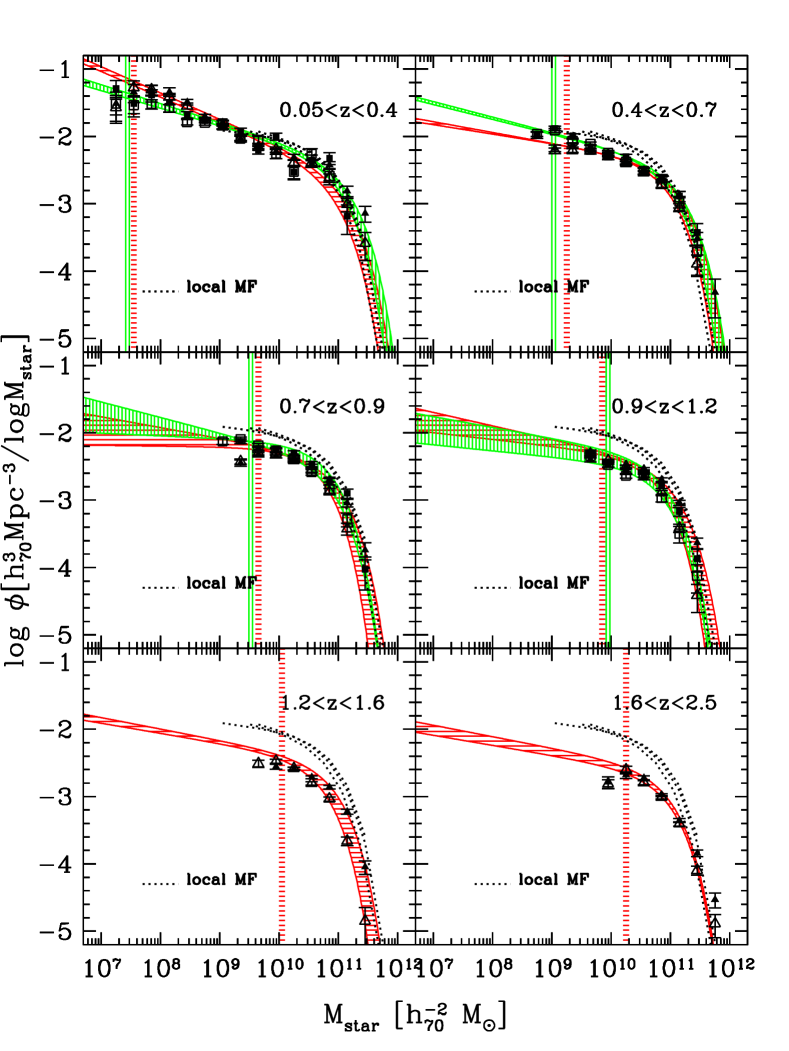
Figure 9: Galaxy Stellar Mass Functions in the $I$-selected (squares) and $K$-selected (triangles) using both methods to estimate the stellar masses (empty symbols for smooth SFHs and filled for complex SFHs). The STY Schechter fits for the 2 methods limit the hatched regions (horizontal hatched for the $K$-selected and vertical hatched for the $I$-selected samples). Vertical hatched regions represents the completeness limit of the 2 samples. The local MFs by Cole et al. (2001), both original and “rescaled” version (Fontana et al. 2004), and by Bell et al. (2003) are reported in each panel as dotted lines.

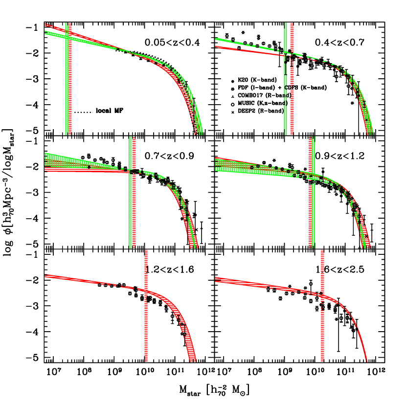
Figure 10: Comparison between the $I$-selected and the $K$-selected MFs in the VVDS (hatched vertical and horizontal STY regions, respectively, see caption Figure 9) and the literature data (K20, COMBO17, MUSIC, DEEP2, FDF+CDFS; for each the band of selection is indicated in the parenthesis). The vertical hatched regions represent the completeness limits of the VVDS samples.

For the galaxies in the $I$-selected sample not covered by near-IR data, we have used the statistically corrected masses derived through a Monte Carlo simulation, to take into account the effect of the near-IR photometry in the mass determination (see Sec. 3.3). Figure 7 shows the effect in the MF for complex SFHs. The high mass tail is significantly reduced if we use statistically corrected masses when near-IR is not available. Consistent MFs have been obtained in the sub-area of $I$-selected sample where near-IR photometry is available (see Fig. 7).

For the $K$-selected sample, we have analyzed the effect of the cosmic variance on small areas, deriving the MF for the two $K$-selected subsamples, deep and shallow, separately (see Figure 8). We find a significantly lower MF (by a factor 1.8 and 1.6) in the redshift range $0.4<z<0.7$ and $0.7<z<0.9$ in the deep $K$-selected sample ($K<22.84$ over 168 arcmin²) compared to the shallow $K$-band sample ($K<22.34$ over 442 arcmin²). The significance of such differences in the MF, is of $\sim 2-3\sigma$ in each mass bin at $0.4<z<0.7$ and $\sim 1-2\sigma$ at $0.7<z<0.9$. Globally, i.e. for the total number densities over the complete mass range, the differences are significant at about 5-3 $\sigma$ level in the two redshift ranges, respectively. This problem leads to a clear warning on the results based on small fields, as covered by most of the previous existing surveys.

In Figure 9 we show the MFs derived using the $I$-selected spectroscopic sample and the $K$-selected photometric sample for both methods (smooth and complex SFHs) to derive the masses. The resulting mass functions are quite well fitted by Schechter functions. The best-fit Schechter parameters are summarized in Table 2, with the uncertainties derived from the projection of the 68% confidence ellipse. Since in the lowest and highest redshift bins ($z\simeq 0.2$ and $2$) the values of ${\cal M}_{\rm stars}^{*}$ and the low-mass-end slope ($\alpha$), respectively, are poorly constrained, they have been fixed to the values measured in the following and previous redshift bins respectively.

We note, first, that the overall agreement between the MF derived with the different methods for masses determination is fairly satisfactory, albeit complex SFHs estimates provide typically larger masses. The systematic shift between the 2 methods (Section 3.4) is reflected in most of the redshift bins also in the characteristic mass (${\cal M}_{\rm stars}^{*}$) of the MF while the best fit slopes ($\alpha$) and $\phi^{*}$ Schechter parameters agree within the errors between the different methods in most of the redshift bins.

We note, furthermore, an overall agreement between the 2 samples ($I$- and $K$-selected), and in most of the redshift bins the Schechter parameters agree within the errors, even if some differences exist. More in detail, the $I$-selected sample in the range $0.4<z<0.9$ has a higher low-mass ($<9.5$ dex) end and a slightly steeper MF ($\alpha\sim-1.23$) than the $K$-selected one ($\alpha>-1.15$). These differences are probably due to the population of blue $K$-faint galaxies, that are missed in the $K$-sample, as discussed in Section 3. These galaxies have, indeed, median colours in the $I$-selected sample that are bluer than in the $K$-selected sample ($I-K\simeq 0.45$ compared to $\simeq 0.89$). A similar behaviour has been noted in the local MF derived using an optically selected sample ($g$ band) compared to the local MF from the near-IR (2MASS) sample (Bell et al. 2003). On the contrary, at even lower masses ($<8.5$ dex) at $z<0.4$ the $K$-selected MF is slightly steeper than the $I$-selected one, but no significant differences in the colour of the two populations is found.

4.2 Comparison with Previous Surveys

In general, previous efforts to derive MF have relied on smaller or more limited samples, or often based mainly on photometric redshifts (Drory et al. 2004, 2005). We have compared our MF determination with literature results based on different surveys (K20, COMBO17, MUSIC, DEEP2, FDF+CDFS), rescaled to Chabrier IMF (see Figure 10). Our MFs rely on a higher statistics at intermediate to high-mass ranges, and therefore present lower statistical errors. At $z<0.2$ we sample unprecedented mass ranges, more than one order of magnitude lower than previous surveys, while at $z>0.4$ the FDF and MUSIC surveys reach lower mass limits even if on significantly smaller area. Our MFs are in fairly good agreement with previous studies over the whole mass range up to $z\sim 1.2$. However, some differences exist, in particular at the massive end, which is more sensitive to the different selections, methods, statistics and to cosmic variance due to large scale structures: for example, in the MUSIC-GOODS survey there are two significant overdensities at $z\sim 0.7$. The MFs from COMBO17 (Borch et al. 2006) and also from DEEP2 (Bundy et al. bun06 (2006)) are systematically higher than previous surveys at the massive-end, in particular in the range $0.7<z<1.2$. The MFs in the FDF+CDFS are instead systematically lower than ours at the massive-end and higher than our extrapolation to masses lower than our completeness limit. At $z>1.2$ our MF is systematically higher than previous studies. Given the area sampled (more than a factor 4 wider compared to FDF+CDFS and to MUSIC) and the consistency at these redshifts of our MF in the 2 $K$-selected separated areas (see Figure 8), we are confident in our results. However at high-$z$ the uncertainties on the stellar masses estimate increase (up to $0.16$ dex including also the photometric redshift errors) and could produce a partially spurios excess in the number densities of galaxies, in particular in the massive tail of the MF. This effect is discussed in Kitzbichler & White (2007) which take into account in the hierarchical formation Millenium simulation the effect of the dispersion in the mass determination (0.25 dex, i.e. 78%). We have performed a similar analysis, taking into account the uncertainty on the mass, due to the fitting technique ($\sim 30\%$) and to the uncertainty of the photometric redshifts (both its dependence on redshift and magnitudes as described in previous sections, i.e. up to $\sigma_{z}\simeq 0.2$ at $z=2$ and $K>21.5$). We found that the effect on the MF is always small, and only the very massive tail ($M>2\times 10^{11}M_{\odot}$) is systematically overestimated (up to 0.2 dex). This effect can not completely explain the excess found compared to previous surveys, which are affected in a similar way by the same bias.

4.3 The Evolution of the Galaxy Stellar Mass Function

The VVDS allows us to follow the evolution of the MF within a single sample over a wide redshift range. Difficulties in the interpretation of the evolution are, indeed, due to the comparison with the local MFs, which have been determined with different methods and sample selection. For example, no local MF has been derived using complex SFHs for mass determinations. In our analysis we use, as reference, the local MF by Bell et al. (2003) and Cole et al. (2001) rescaled to Chabrier IMF. In particular, the Cole et al. (2001) local mass function, derived with smooth SFHs but with formation redshift fixed at $z=20$, has been rescaled to smooth SFHs method with free formation redshift by Fontana et al. (2004).

The first important result is that, thanks to our very deep samples, both $I$- and $K$-selected, the low-mass end of the MF is even better determined than in the local sample up to $z<0.4$, probing for the first time masses down to about $3\times 10^{7}M_{\odot}$. The low mass-end is rather steep ($-1.38<\alpha<-1.26$), and could even be described by a double Schechter function, and is steeper than the local estimates ($\alpha=-1.18\pm 0.03$ Cole et al. 2001, $\alpha=-1.10\pm 0.02$ Bell et al. 2003), possibly due to the fact they are not probing masses smaller than $10^{9}$ M_⊙ (more than one order of magnitude more massive than in our sample). As evident from Figure 9, we find a substantial population of low-mass ($<10^{9}\,M_{\odot}$) galaxies at low redshifts ($z<0.4$). This population is composed by faint blue galaxies with similar properties in the 2 samples ($I$- and $K$-selected): $I,K\simeq 22-23$, $M_{I},M_{K}\simeq-16,-17$ with median $M_{I}-M_{K}\simeq 0.3$, and median $z\simeq 0.1-0.2$. This is a very strong result from our survey which can rely on a wider area and a deeper sample than previous surveys at low redshifts. At $z>0.4$ the low-mass slope is on the contrary always consistent with the local values. Even if we are not probing masses smaller than $10^{8}M_{\odot}$ at $z>0.4$, we found that the MF remains quite flat ($-1.23<\alpha<-1.04$) at all redshifts, similar to that of Fontana et al. (2006) which probe lower masses (see figure 10).

From a visual inspection of Figure 9, we see that up to $z\sim 0.9$ there is only a weak evolution of the MF, as suggested by previous results (Fontana et al. 2004, 2006, Drory et al. 2005), while at higher redshifts there appears to begin a decrease in the normalization of the MF, even if a massive tail remains present up to $z=2.5$. At intermediate masses ($9.5<\log M<10.5$), our VVDS MF is very well defined and shows a clear evolution, i.e. the number density decreases with increasing redshifts compared to both the first VVDS redshift bin and the local MF. This evolution is quite mild up to $z\simeq 0.9$, while it becomes faster at higher $z$. At larger masses the high mass end of the MF ($>10^{11}\,M_{\odot}$) shows a small evolution up to $z\simeq 2.5$. However, its evolution is extremely dependent on the assumed local MF and on the uncertainties in the mass determination, which produce a larger dispersion between the different methods and samples compared to the intermediate-mass range.

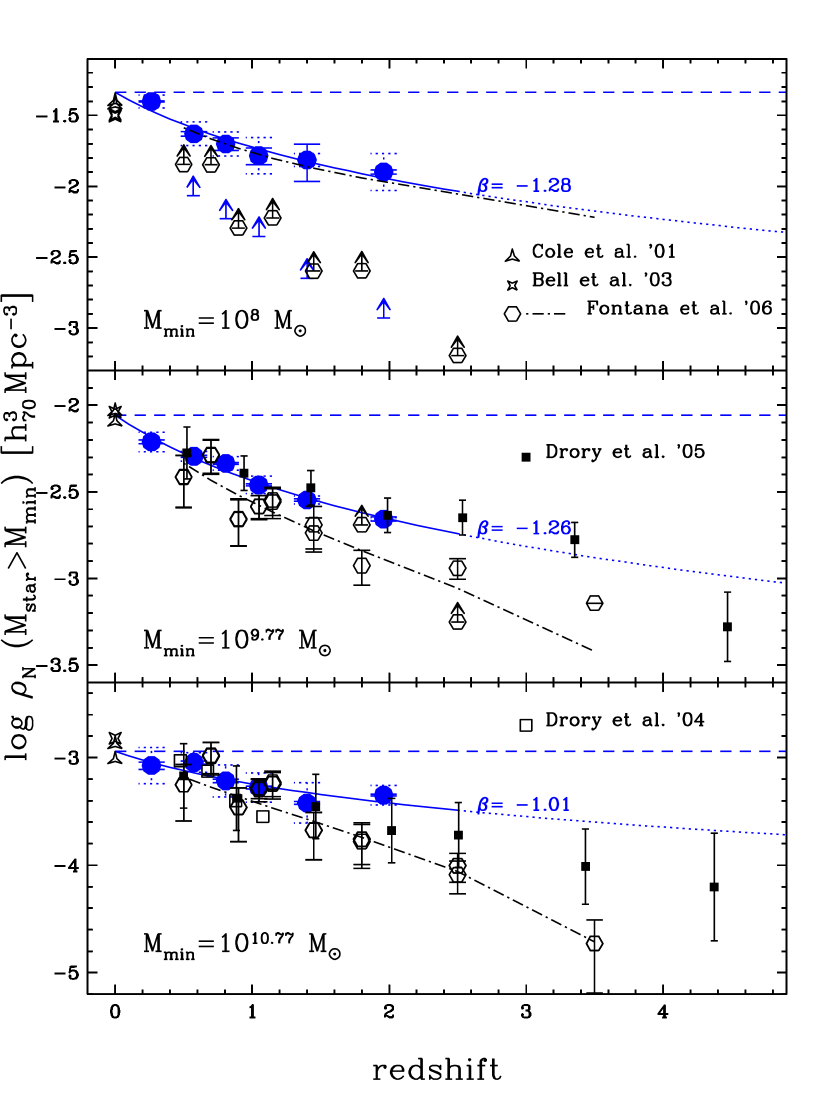
Figure 11: Cosmological evolution of the galaxy number density as a function of redshift, as observed from the VVDS in various mass ranges ($>10^{8}M_{\odot}$, $>10^{9.77}M_{\odot}$ and $>10^{10.77}M_{\odot}$ from top to bottom). Observed data from $V_{\rm max}$ (shown as lower limit in the top panel) have been corrected, when necessary, for incompleteness integrating the mass function using the best fit Schechter parameters. VVDS data (big filled circles), averaged over the $I$- and the $K$-selected samples and the 2 methods to derive the mass, are plotted along with their statistical errors (solid error bars) and the scatter between the 2 different samples and methods (dotted error bars). The solid lines show the best-fit power laws $\propto(1+z)^{\beta}$, while the dashed lines correspond to the no-evolution solution normalized at $z=0$. Results from previous surveys (small points and dot-dashed lines) are also shown.

In order to quantify the MF evolution, and its mass dependency independently from the local MF, in the next section we derive number densities for different mass limits.

4.4 Galaxy Number Density

Here we derive the number density of galaxies as a function of redshift, using different lower limits in mass (${\cal M}_{\rm min}$). We have estimated the number density from the observed data (from $V_{\rm max}$), as well as from the incompleteness-corrected MFs, i.e. integrating the best-fit Schechter functions over the considered mass range. The corrections due to faint galaxies dominate for ${\cal M}_{\rm min}=10^{8}M_{\odot}$, while they are negligible for the other mass limits considered. A formal uncertainty in this procedure was estimated by considering the $V_{\rm max}$ statistical errors and the range of acceptable Schechter parameters values. In Figure 11 we plot our VVDS determinations, averaged over the $I$- and $K$-selected samples and the 2 methods for mass determination (listed in Table 3), along with their statistical errors (always less than 10%) and the scatter between the 2 different samples and methods (ranging between 10 and 45% and due mainly to the different methods rather than to the different samples). With the two methods we find similar trends with redshift of the number densities of galaxies, but with a systematic shift which is significant only for the highest mass limit (for complex SFHs the galaxy number densities are $\sim 50$% higher than for smooth SFHs). The effect of photometric redshift and mass uncertainty on the number densities is always small ($<15\%$) for the mass range shown in Figure 11, except for the very massive galaxies ($>2\times 10^{11}$ $M_{\odot}$, not shown in the figure because of the small number of galaxies in this mass range) where the intrinsic values could be up to a factor $\sim 2$ lower (see discussion in section 4.2). The decrease in number density with redshift for all the adopted mass limits is evident.

Table 3: Number Density and Stellar Mass Density

$z_{inf}$

$z_{sup}$

Log($\rho_{N}$)

Scatter

Error

Log($\rho_{\rm stars}$)

Scatter

Error

log(${\cal M}_{\rm stars}$)$>8$

0.05	0.40	-1.40	0.04	0.01	8.45	0.09	0.01
0.40	0.70	-1.63	0.08	0.02	8.34	0.08	0.02
0.70	0.90	-1.70	0.08	0.04	8.22	0.11	0.01
0.90	1.20	-1.78	0.13	0.05	8.14	0.12	0.01
1.20	1.60	-1.81	0.05	0.11	8.04	0.14	0.02
1.60	2.50	-1.90	0.13	0.01	8.05	0.11	0.01

log(${\cal M}_{\rm stars}$)$>9.77$

0.05	0.40	-2.20	0.06	0.01
0.40	0.70	-2.29	0.03	0.01
0.70	0.90	-2.33	0.04	0.01
0.90	1.20	-2.45	0.05	0.01
1.20	1.60	-2.54	0.02	0.01
1.60	2.50	-2.65	0.01	0.01

log(${\cal M}_{\rm stars}$)$>10.77$

0.05	0.40	-3.07	0.18	0.05	8.00	0.22	0.04
0.40	0.70	-3.04	0.10	0.02	8.04	0.14	0.02
0.70	0.90	-3.22	0.16	0.02	7.80	0.19	0.02
0.90	1.20	-3.28	0.15	0.02	7.76	0.18	0.02
1.20	1.60	-3.42	0.23	0.02	7.59	0.28	0.02
1.60	2.50	-3.35	0.11	0.01	7.70	0.11	0.01

We have compared VVDS results to previous surveys and with different local determinations. For the total number density ($10^{8}<{\cal M}_{\rm stars}<10^{13}M_{\odot}$) VVDS data are very well consistent with the evolutionary STY fit determined by Fontana et al. (2006) in the GOODS-MUSIC survey. At intermediate masses ($>10^{9.77}M_{\odot}$, corresponding to $10^{10}M_{\odot}$ for Salpeter IMF) our VVDS data have a better determination and smaller uncertainties than previous ones and are consistent with most of them at $z<1.2$ and in the upper envelope at higher $z$. For the high mass range ($>10^{10.77}M_{\odot}$, corresponding to $10^{11}M_{\odot}$ for Salpeter IMF) we are quite consistent with previous results, and even if our VVDS have lower errors than previous ones, the dispersion within the various VVDS measurements reflect the uncertainties for massive galaxies.

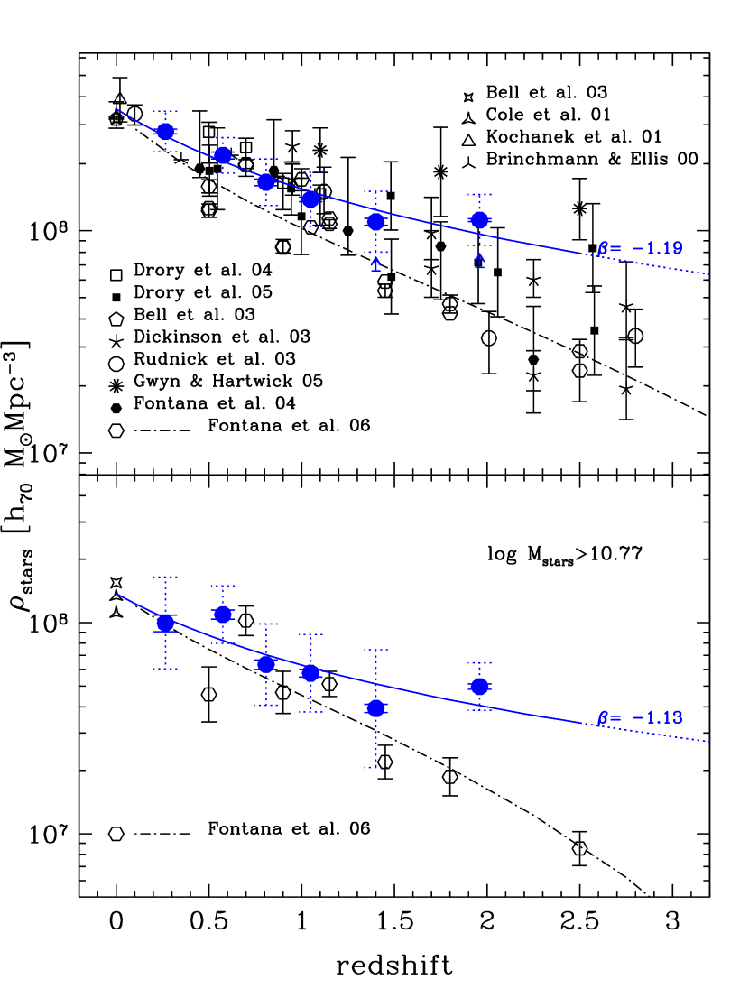
Figure 12: Cosmological evolution of the stellar mass density as a function of redshift as observed from the VVDS for 2 mass ranges: integrated over the whole range $10^{8}M_{\odot}\leq{\cal M}_{\rm stars}\leq 10^{13}M_{\odot}$ (upper panels) and for massive galaxies ($>10^{10.77}M_{\odot}$) (lower panels). Symbols and lines as in Figure 11.

If we represent the average number density evolution by a power law $\rho_{N}\propto(1+z)^{\beta}$, we find that $\beta({\cal M}_{\rm stars}>10^{8})=-1.28\pm 0.15$, $\beta({\cal M}_{\rm stars}>10^{9.77})=-1.26\pm 0.10$, and $\beta({\cal M}_{\rm stars}>10^{10.77})=-1.01\pm 0.05$ (the errors on $\beta$ represent the uncertainties due to the 2 different methods). We find on average a similar evolution for the 2 methods analyzed and a slightly milder evolution with increasing mass limit (‘downsizing’ in mass assembly). The average evolution from $z=0$ to $z=1$ is a factor $2.4\pm 0.3$ and $2.0\pm 0.1$ from low to high-mass galaxies, respectively, and increases to a factor $4.0\pm 0.9$ and $3.0\pm 0.2$, respectively, at $z=2$. We note moreover that for the highest mass limit (${\cal M}_{\rm stars}>10^{10.77}$) at low redshift ($z<0.7$) the number density observed is consistent with no-evolution (fixing the value to $z=0$ we found an evolution $<30\%$), excluded instead for the intermediate and low-mass limit. At high-$z$ ($z>1.5$) for intermediate and high-mass range we note a flattening in the number density from the VVDS data, similar to Drory et al. (2005), but higher than Fontana et al. (2006). This flattening is due to the high mass tail observed in the range $1.6<z<2.5$. This population shows extremely red colours ($M_{I}-M_{K}\simeq 0.8$) and could be related to the appearance of a population of massive star forming dusty galaxies, observed in previous surveys (Fontana et al. 2004, Daddi et al. 2004b). The small excess induced by uncertainties on the mass and photometric redshifts (see discussion in section 4.2) can not completely explain the difference with Fontana et al. (2006) survey, which is affected by the same bias in a similar way.

The mass dependent evolution (“mass downsizing”) is very debated and the results from different surveys are still controversial. Deep surveys, such as the FDF & CDFS (analyzed by Drory et al. 2005) find an evolution consistent with ours (a decrease of about a factor 2.5 – 4 at $z=1-2$ in the number density of galaxies $>10^{10.77}\,M_{\odot}$). Fontana et al. (2006) suggest a similar mild evolution up to $z=1$, for massive galaxies ($>10^{10.77}\,M_{\odot}$) and a stronger evolution at $z>1.5$, reaching a factor about 10 at $z=3$. Similarly, Cimatti et al. (2006) show that the number density of luminous (massive, ${\cal M}_{\rm stars}>10^{11}\,M_{\odot}$) early-type galaxies is nearly constant up to $z\sim 0.8$, while Bundy et al. (2006) find a slight decrease, consistent with no evolution, only for even more massive system ($>3\times 10^{11}\,M_{\odot}$) and a more significant decline for ${\cal M}_{\rm stars}<3\times 10^{11}\,M_{\odot}$. Vice versa, data from the MUNICS survey (Drory et al. 2004) show a faster evolution of massive galaxies, even faster than for the less massive systems (see also Figure 4 in Drory et al. 2005).

To summarize, our accurate results show that the MF evolves mildly up to $z\simeq 1$ (about a factor 2.5 in the total number density) and that a high-mass tail is still present up to $z=2.5$. Moreover, we find that massive systems show an evolution that is on average milder ($<50$% at $z<1$) than intermediate and low-mass galaxies and consistent with a mild/negligible evolution ($<30$%) up to $z\sim 0.8$. Conversely, a no-evolution scenario in the same redshift range is definitely excluded for intermediate- and low-mass galaxies.

This behaviour suggests that the assembly of the stellar mass in objects with mass smaller than the local ${\cal M}_{\rm stars}^{*}$ was quite significant between $z=2$ and $z=0$. Qualitatively, this behaviour is expected for galaxies with SFHs prolonged over cosmic time, which therefore continue to grow in terms of stellar mass after $z\sim 1$. Conversely, our results further strengthen the fact that the number density of massive galaxies is roughly constant up to $z\simeq 0.8$, consistently with a SFH peaked at higher redshifts, with the conversion of most of their gas into stars happening at $z>1.5-2$, ruling out the ‘dry mergers’ as the major mechanism of their assembly history, below $z<1$.

5 Mass Density

Various attempts to reconstruct the cosmic evolution of the stellar mass density have been previously made, mainly using NIR-selected samples (Dickinson et al. 2003, Fontana et al. 2004, Drory et al. 2005). Our survey offers the possibility to investigate it using the MF derived from two different optical- and NIR-selected samples, taking advantage of our depth, and relatively wide area covered. Furthermore, the different methods analyzed here to derive the stellar mass content give us a direct measure of the uncertainties involved.

We have estimated the stellar mass density from the observed data, as well as from the incompleteness-corrected MFs. Up to $z<1$ the corrections due to faint galaxies are relatively small. A formal uncertainty in this procedure was estimated by considering the $V_{\rm max}$ statistical errors and the range of acceptable Schechter parameters values.

Figure 12 shows our results (averaged over the $I$- and $K$-selected samples and the 2 methods with a typical scatter of about 30-50% and statistical errors always less than 5% see Table 3), for the total mass density and for the density in massive galaxies ($>10^{10.77}$), along with their representative power laws ($\rho_{\rm stars}\propto(1+z)^{\beta}$), and compared to literature data (see references in the figure). For the total mass density, even if the results from our survey cover a range of values with some significant differences between the two different methods (up to $\sim 40$%), the general behaviour and evolutionary trend is well defined by $\beta=-1.19\pm 0.05$. We find that the evolution of the stellar mass density is relatively slow with redshift, with a decrease of a factor $2.3\pm 0.1$ up to $z\simeq 1$, up to a factor $4.5\pm 0.3$ at $z=2.5$. The agreement of average total mass density with previous surveys is reasonably good, and the range covered by VVDS data reflect the different selection techniques and methods used in different surveys. The average total mass density evolution is milder than in the MUSIC sample (Fontana et al. 2006) already at $z>0.5$. Our evolutionary trend is consistent with the upper envelope of previous surveys, even if our highest-redshift value is uncertain because the low-mass slope is poorly constrained. For comparison the analysis of VVDS data using a IRAC-selected sample (see Arnouts et al. 2007) finds similar values for the mass density, except that the highest redshift point is lower than ours. Given the present uncertainties on the low-mass slope of the GSMF, the total mass density at $z\simeq 2$ remains poorly constrained.

The mass density of high-mass objects ($>10^{11}M_{\odot}$ with Salpeter IMF) varies by a factor up to $1.8$ within the 2 methods adopted, but the evolutionary trend is similar ($\beta=-1.13\pm 0.01$) and consistent with a decrease of about a factor $2.18\pm 0.02$ to $z=1$ and $3.44\pm 0.04$ to $z=2.0$. Moreover at low redshift ($z<0.7$) the VVDS observed data are consistent with a mild/negligible evolution ($<30$%), as indicated by the number density of massive galaxies (see previous Section). Our data are roughly consistent with Fontana et al. (2006) up to $z=1.5$ (even if the slope of the evolutionary trend is shallower), while at $z>1.5$ the VVDS mass-density of massive galaxies is significantly higher than that in Fontana et al. (2006), reflecting the excess in MF at high-$z$ noted in the VVDS MF compared to previous ones (see Section 4.2). This results, therefore, in a flatter evolutionary trend over the total redshift range. Given the wider area and completeness for high-mass objects, our samples guarantee a higher statistical accuracy and confidence level than before. However some caveat remains due to the effect of photometric redshift and mass uncertainty on the mass densities, which is anyhow always small ($<15\%$) except for the massive galaxies ($>6\times 10^{10}$ $M_{\odot}$) where the intrinsic values could be up to 20-30% lower than our estimates (see discussion in Section 4.2).

6 Summary and Discussion

We have investigated the evolution of the Galaxy Stellar Mass Function up to to $z=2.5$ using the VVDS survey covered by deep VIMOS spectroscopy ($17.5<I<24$) and multiband photometry (from $U$ to $K$-band). For our analysis we have used two different samples: (1) the optical ($I$-selected, $17.5<I<24$) main spectroscopic sample, based on about 6500 secure redshifts over about 1750 arcmin², and (2) a near-IR sample ($K$-selected, $K<22.84$ & $K<22.34$), in a sub-area of about 610 arcmin² and based on about 10200 galaxies with accurate photometric and spectroscopic redshifts. For the first time we have probed masses down to a very low limit, in particular at low-$z$ (down to $\sim 3\times 10^{7}M_{\odot}$ at $z\sim 0.2$), while the relatively wide area has allowed us to determine the MF with much higher statistical accuracy than previous samples.

In order to better understand uncertainties we have applied and compared two methods to estimate the stellar mass content in galaxies from multiband SED fitting. The 2 methods differ in the explored parameter space (metallicity, dust law and content) and are based on different assumptions on previous star formation history. The main results from the stellar mass estimate can be summarized as follows:

• The agreement between the 2 methods is fairly good even if masses estimated with ‘complex SFHs’ are systematically higher than ‘smooth SFHs’ masses. For the $K$-selected sample the mean difference is $\langle d\log{\cal M}_{\rm stars}\rangle\simeq 0.12$ dex, and the dispersion is $\sigma=0.13$. The differences are mainly due to the secondary burst component (complex SFHs) compared to smooth SFHs.

• We found that mass estimates using only optical bands are in rather good agreement with those using also NIR bands up to $z\sim 1.2$. We have used this information to statistically correct masses for objects without near-IR photometry. At higher redshifts the shift and dispersion dramatically increase and the mass estimates become unreliable if near-IR photometry is not available.

We have, thus, derived the MF using the VVDS $I$-selected sample and extended it up to $z=2.5$ thanks to the $K$-selected sample. From a detailed analysis of the MF, galaxy number density and mass density, in different mass ranges, through cosmic time, we found evidences for:

• a substantial population of low-mass galaxies ($<10^{9}M_{\odot}$) at $z\simeq 0.2$ composed by faint ($I,K\simeq 22,23$) blue galaxies with median $M_{I}-M_{K}\simeq 0.3$, and absolute magnitudes $M_{I},M_{K}\simeq-16,-17$;

• a slow evolution of the stellar mass function with redshift up to $z\sim 0.9$ and a faster evolution at higher-$z$, in particular for less massive systems. A massive population is present up to $z=2.5$ and have extremely red colours ($M_{I}-M_{K}\simeq 0.7-0.8$).

• at $z>0.4$ the low-mass slope of the GSMF does not evolve significantly and remains quite flat ($-1.23<\alpha<-1.04$).

• the number density shows, on average, a mild differential evolution with mass, which is slower with increasing mass limit. Such evolution can be described by a power law $\propto(1+z)^{\beta(>M)}$. Within the VVDS redshift range we found that $\beta(>10^{8}\,M_{\odot})=-1.28\pm 0.15$, $\beta(>10^{9.77}\,M_{\odot})=-1.26\pm 0.10$ and $\beta(>10^{10.77}\,M_{\odot})=-1.01\pm 0.05$. For massive galaxies at low redshift ($z<0.7$) the evolution is consistent with mild/negligible-evolution ($<30$%), which is excluded for low-mass systems.

• the evolution of the stellar mass density is relatively slow with redshift, with a decrease of about a factor $2.3\pm 0.1$ to $z\simeq 1$, while at $z\simeq 2.5$ the decrease amounts to a factor up to $4.5\pm 0.3$, milder than in previous surveys. For massive galaxies the evolution at low redshift ($z<0.7$) is consistent with a mild/negligible evolution($<30\%$), and shows a flattening compared to previous results at $z>1.5$ due to a population with extremely red colours.

Our results provide new clues on the controversial question of when galaxy formed and assembled their stellar mass. Most of the massive galaxies seem to be in place up to $z=1$ and have, therefore, formed their stellar mass at high redshift ($z>1$), rather than assembled it mainly through continuous galaxy merging of small galaxies at $z<1$. On the contrary, less massive systems have assembled their mass (through merging or prolonged star formation history) later in cosmic time. In agreement with our results, a substantial population of high-$z$ ($z\sim 2-3$) dusty and massive objects have been discovered in near-IR surveys (Daddi et al. 2004b) and detected by Spitzer in the far-IR (Daddi et al. 2005, Caputi et al. 2006b). This population could be related to the initial phase of massive galaxy formation during their strong star forming and dusty phase.

Finally, our results are not completely accounted for by most of theoretical models of galaxy formation (see Fontana et al. 2004, 2006 and Caputi et al. 2006a for a detailed comparison with models). For instance, models by De Lucia et al. (2006) predict that the most massive galaxies generally form their stars earlier, but assemble them later, mainly at $z<1$ via merging, than the less massive galaxies (i.e. ’downsizing in star formation but ’upsizing’ in mass assembly, see Renzini 2007 for a recent discussion). Furthermore, the stronger decrease with redshift of the low-mass population, with a low-mass end of the GSMF which remains substantially flat up to high redshift, is not reproduced by most of the theoretical galaxy assembly models, which tend, indeed, to overpredict the low-mass end of the MF (see Fontana et al. 2006).

Understanding the mass assembly of less massive objects and disentangling merging processes from prolonged star formation history is more complicated. In this respect for a better comprehension of galaxy formation the VVDS will allow us to further investigate the evolution of the stellar mass function up to high-$z$ also for different galaxy types (spectral and morphological) and in different environments. For example Arnouts et al. (2007) study the mass density evolution of different galaxy population. Further analysis of galaxy mass dependent evolution, using stellar population properties, as well as observed spectral features, will be presented in forthcoming papers (Lamareille et al., in preparation, Vergani et al. 2007). Furthermore, it will be possible to push the study of the galaxy stellar mass function at higher redshifts using SPITZER mid-IR observations. While most of present studies (Dickinson et al. 2003, Drory et al. 2005) do not use rest-frame near-IR photometry to estimate stellar masses, our VVDS-SWIRE collaboration will allow to combine the deep VVDS spectroscopic sample with SPITZER-IRAC photometry.

References

- (1) Avni, Y, Bahcall, J. N. 1980, ApJ, 235, 694
- (2) Arnouts, S., Walcher, C. J., Le Fevre, O., et al. 2007, A&A, submitted [astro-ph:0705.2438]
- (3) Bell, E. F., de Jong, R. S., 2001, ApJ, 550,212
- (4) Bell, E. F., McIntosh, D. H., Katz, N., & Weinberg, M. D. 2003, ApJS, 149, 289
- (5) Bell, E. F., Wolf, C., Meisenheimer, K., et al. 2004, ApJ, 608, 752
- (6) Bell, E.F.; Phleps, S., Somerville, R. S., et al. 2006, ApJ, 652, 270
- (7) Bertin, E., Arnouts, S. 1996, A&AS, 117, 393
- (8) Bolzonella, M., Miralles, J.-M., Pelló, R. 2000, A&A, 363, 476
- (9) Borch, A., Meisenheimer, K., Bell, E. F., et al. 2006, A&A, 453, 869
- (10) Bower, R. G., Benson, A. J., Malbon, R., et al. 2006, MNRAS, 370, 645
- (11) Brinchmann, J., & Ellis, R. S. 2000, ApJ, 536, L77
- (12) Brinchmann, J., Charlot, S., White, S. D. M., et al. 2004, MNRAS, 351. 1151
- (13) Brown, M. J. I., Dey, A., Jannuzi, B. T., et al., 2007, ApJ, 654, 858
- (14) Bruzual, G., & Charlot, S. 2003, MNRAS, 344, 1000
- (15) Bundy, K., Ellis, R.S., Conselice, C.J., et al. 2006, ApJ, 651, 120
- (16) Calzetti, D., Armus, L., Bohlin, R. C., et al. 2000, ApJ, 533, 682
- (17) Caputi, K. I., McLure, R. J., Dunlop, J. S., Cirasuolo, M., Schael, A. M. 2006a, MNRAS, 366, 609
- (18) Caputi, K. I., Dole, H., Lagache, G., et al. 2006b, ApJ, 637, 727
- (19) Chabrier, G. 2003, PASP, 115, 763
- (20) Charlot, S., & Fall,S. M. 2000, ApJ, 539, 718
- (21) Cimatti, A., Pozzetti, L., Mignoli, M., et al. 2002, A&A, 391, L1
- (22) Cimatti, A., Daddi, E., Renzini, A., et al. 2004, Nature, 430, 184
- (23) Cimatti, A., Daddi, E., Renzini, A., 2006, A&A, 453, L29
- (24) Cole, S., Norberg, P., Baugh, C. M., et al. 2001, MNRAS, 326, 255
- (25) Cowie, L. L., Songaila, A., Hu, E. M., Cohen, J. G. 1996, AJ, 112, 839
- (26) Daddi, E., Cimatti, A., Renzini, A., et al. 2004a, ApJ, 617, 746
- (27) Daddi, E., Cimatti, A., Renzini, A, et al. 2004b, ApJ, 600, L127
- (28) Daddi, E., Renzini, A., Pirzkal, N., et al. 2005, ApJ, 626, 680
- (29) Daddi, E., Alexander, D. M.; Dickinson, Mi, et al., 2007, ApJ, submitted [astro-ph/0705.2832]
- (30) De Lucia, G., Springel, V., White, S. D. M., Croton, D., & Kauffmann, G. 2006, MNRAS, 366, 499
- (31) De Lucia, G., Blaizot, J., 2007, MNRAS, 375, 2
- (32) Dickinson, M., Papovich, C., Ferguson, H. C., & Budavári, T. 2003, ApJ, 587, 25, D03
- (33) di Serego Alighieri, S., Vernet, J., Cimatti, A., et al. 2005, A&A, 442, 125
- (34) Drory, N., Feulner, G., Bender, R., et al. 2001, MNRAS, 325, 550
- (35) Drory, N., Bender, R., Feulner, G., et al. 2004, ApJ, 608, 742
- (36) Drory, N., Salvato, M., Gabasch, A., et al. 2005, ApJ, 619, L131
- (37) Faber, S. M., Willmer, C. N. A., Wolf, C., et al. 2005, ApJ, submitted [astro-ph/0506044]
- (38) Felten, J. E. 1976, ApJ, 207, 700
- (39) Fioc, M., Rocca-Volmerange, B., 1997, A&A, 326, 950
- F (03) Fontana, A., Donnarumma, I., Vanzella, E., et al. 2003, ApJ, L594, 9, F03
- (41) Fontana, A., Pozzetti, L., Donnarumma, I., et al. 2004, A&A, 424, 23, F04
- (42) Fontana, A., Salimbeni, S., Grazian, A., et al. 2006, A&A, 459, 745
- (43) Franzetti, P., Scodeggio, M., Garilli, B., et al. 2007, A&A, 465, 711
- (44) Gallazzi, A., Charlot, S., Brinchmann, J., White, S. D. M., & Tremonti, C. 2005, MNRAS, 362, 41
- (45) Gavazzi, G., Pierini, D., & Boselli, A. 1996, A&A, 312, 397
- (46) Glazebrook, K.; Abraham, R. G.; McCarthy, P. J., et al. 2004, Nature, 430, 181
- (47) Gould, A., Bachall, J.N. & Flynn, C. 1996, ApJ, 465, 759
- (48) Ilbert, O., Tresse, L., Arnouts, S., et al. 2004, MNRAS, 351, 541
- (49) Ilbert, O., Tresse, L., Zucca, E., et al. 2005, A&A, 439, 863
- (50) Ilbert, O., Arnouts, S., McCracken, H. J., et al. 2006, A&A, 457, 841
- (51) Iovino, A., McCracken, H. J., Garilli, B., et al. 2005, A&A, 442, 423
- (52) Kang, X., Jing, Y. P., & Silk, J., 2006, ApJ, 648, 820
- (53) Kauffmann, G., Heckman, T. M., White, S. D. M., et al. 2003, MNRAS, 341, 33
- (54) Kitzbichler, M. G., White, S. D. M., 2007, MNRAS, 376, 2
- (55) Kranz, T., Slyz, A., Rix, H.-W. 2003, ApJ, 586, 143
- (56) Kriek, M., van Dokkum, P. G., Franx, M., et al., 2007, ApJ, accepted [astro-ph/0611724]
- (57) Kroupa, P. 2001, MNRAS, 322, 231
- (58) Le Fèvre, O., Saisse, M., Mancini, D., et al. 2003a, SPIE, vol. 4841, p.1670
- (59) Le Fèvre, O., Mellier, Y., McCracken, H. J., et al. 2004, A&A, 417, 839
- (60) Le Fèvre, O., Vettolani, G., Garilli, B., et al. 2005, A&A, 439, 845
- (61) Le Fèvre, O., Vettolani, G., Maccagni, D. et al. 2003b, proc. of IAU Symp. 216, Maps of the Cosmos, Sydney, July 2003, M.Colless & L.Staveley-Smith eds. [astro-ph/0311475]
- (62) Lin, L., Koo, D. C., Willmer, C. N. A., et al., 2004, ApJ, 617, 9L
- (63) Madau, P., Pozzetti, L., & Dickinson, M. 1998, ApJ, 498, 106
- (64) Maraston, C., 2005, MNRAS, 362, 799
- (65) Maraston, C., Daddi, E., Renzini, A., et al. 2006, ApJ, 652, 85
- (66) McCracken, H.J., Radovich, M., Bertin, E., et al. 2003, A&A, 410, 17
- (67) Menci, N., Fontana, A., Giallongo, E., et al. 2006, ApJ, 647, 753
- (68) Monaco, P, Fontanot, F., Taffoni, G., 2007, MNRAS, 375, 1189
- (69) Neistein, E.; van den Bosch, F.C., Dekel, A., 2006, MNRAS, 372, 933xN
- Papovich et al. (2001) Papovich, C., Dickinson M.M., Ferguson, H.C., 2001, ApJ, 559, 620
- Papovich et al. (2006) Papovich, C., Moustakas, L. A., Dickinson M.M., et al. 2006, ApJ, 640, 92
- (72) Pozzetti, L., Cimatti, A., Zamorani, G., et al. 2003, A&A, 402, 837
- (73) Radovich, M., Arnaboldi, M., Ripepi, V., et al. 2004, A&A, 417, 51
- (74) Renzini, A. 2005, in IMF50: The Initial Mass Function 50 Years Later, ed. E. Corbelli, F. Palla & H. Zinnecker (Dordrecht: Kluwer) [astro-ph/0410295]
- (75) Renzini, A. 2007, in ’At the Edge of the Universe: Latest Results from the Deepest Astronomical Surveys’, ed. by J. Afonso, ASP Conf. Ser. [astro-ph/0702148]
- (76) Salim, S., Charlot, S., Rich, R. M., et al. 2005, ApJ, 619, L39
- (77) Salpeter, E. E. 1955, ApJ, 121, 161
- (78) Sandage, A., Tammann, G.A., & Yahil, A., 1979, ApJ, 232, 352
- (79) Saracco, P., Longhetti, M., Giallongo, E., et al. 2004, A&A, 420, 125
- (80) Saracco, P., Longhetti, M., Severgnini, P., et al. 2005, MNRAS, 357, L40
- (81) Schechter, P. 1976, ApJ, 203, 297
- (82) Schmidt, M. 1968, ApJ, 151, 393
- (83) Scodeggio, M., Franzetti, P., Garilli, B., et al. 2005, PASP, 117, 1284
- Shapley et al. (2001) Shapley, A. E., Steidel, C. C., Adelberger, K. L., et al. 2001, ApJ 562, 95
- Shapley et al. (2005) Shapley, A. E., Steidel, C. C., Erb, D. K., et al. 2005, ApJ 626, 698
- Somerville et al. (2004) Somerville, R. S., Moustakas, L. A., Mobasher, B., et al. 2004, ApJ, 600, L135
- (87) Strazzullo, V., Rosati, P., Stanford, S. A., et al. 2006, A&A, 450, 909
- (88) Trujillo, I., Feulner, G., Goranova, Y., et al. 2006, MNRAS, 373, L36
- (89) van Dokkum, P. G. 2005, AJ, 130, 2647
- (90) Vergani, D., Scodeggio, M., Pozzetti, L., et al. 2007, A&A, submitted [astro-ph:0705.3018]
- (91) Wolf, C., Meisenheimer, K., Rix, H.-W., et al., 2003, A&A, 401, 73
- (92) Zanichelli, A., Garilli, B., Scodeggio, M., et al. 2005, PASP, 117, 1271
- (93) Zoccali, M., Cassisi, S., Frogel, J. A., et al. 2000, ApJ, 530, 418
- (94) Zucca, E., Ilbert, O., Bardelli, S., et al. 2006, A&A, 455, 879