An adaptive numerical method for the Vlasov equation based on a multiresolution analysis

1 Introduction

Plasmas, which are gases of charged particles, and charged particle beams can be described by a distribution function $f(t,x,v)$ dependent on time $t$, on position $x$ and on velocity $v$. The function $f$ represents the probability of presence of a particle at position $(x,v)$ in phase space at time $t$. It satisfies the so-called Vlasov equation

$$\frac{\partial f}{\partial t}+v\cdot\nabla_{x}f+F(t,x,v)\cdot\nabla_{v}f=0.$$ (1)

The force field $F(t,x,v)$ consists of applied and self-consistent electric and magnetic fields:

$$F=\frac{q}{m}(E_{self}+E_{app}+v\times(B_{self}+B_{app})),$$

where $m$ represents the mass of a particle and $q$ its charge. The self-consistent part of the force field is solution of Maxwell’s equations

$$-\frac{1}{c^{2}}\frac{\partial\mathbf{E}}{\partial t}+\nabla\times\mathbf{B}=\mu_{0}{\mathbf{j}}, \hskip 28.45274pt\nabla\cdot\mathbf{E}=\frac{\rho}{\epsilon_{0}},$$

$$\frac{\partial\mathbf{B}}{\partial t}+\nabla\times\mathbf{E}=0, \hskip 28.45274pt\nabla\cdot\mathbf{B}=0.$$

The coupling with the Vlasov equation results from the source terms $\rho$ and ${\mathbf{j}}$ such that:

$$\rho(t,x)=q\int_{{\mathbb{R}}^{d}}f(t,x,v)\,dv,~{}~{}~{}{\mathbf{j}}=q\int_{{\mathbb{R}}^{d}}f(t,x,v)v\,dv.$$

We then obtain the nonlinear Vlasov-Maxwell equations. In some cases, when the field are slowly varying the magnetic field becomes negligible and the Maxwell equations can be replaced by the Poisson equation where:

$$E_{self}(t,x)=-\nabla_{x}\phi(t,x),\quad-\varepsilon_{0}\Delta_{x}\phi=\rho.$$ (2)

The numerical resolution of the Vlasov equation is usually performed by particle methods (PIC) which consist in approximating the plasma by a finite number of particles. The trajectories of these particles are computed from the characteristic curves given by the Vlasov equation, whereas self-consistent fields are computed on a mesh of the physical space. This method allows to obtain satisfying results with a few number of particles. However, it is well known that, in some cases, the numerical noise inherent to the particle method becomes too important to have an accurate description of the distribution function in phase space. Moreover, the numerical noise only decreases in $\sqrt{N}$, when the number of particles $N$ is increased. To remedy to this problem, methods discretizing the Vlasov equation on a mesh of phase space have been proposed. A review of the main methods for the resolution of the Vlasov equation is given in these proceedings sonnen:enumath .

The major drawback of methods using a uniform and fixed mesh is that their numerical cost is high, which makes them rather inefficient when the dimension of phase-space grows. For this reason we are investigating here a method using an adaptive mesh. The adaptive method is overlayed to a classical semi-Lagrangian method which is based on the conservation of the distribution function along characteristics. Indeed, this method uses two steps to update the value of the distribution function at a given mesh point. The first one consists in following the characteristic ending at this mesh point backward in time, and the second one in interpolating its value there from the old values at the surrounding mesh points. Using the conservation of the distribution function along the characteristics this will yield its new value at the given mesh point. This idea was originally introduced by Cheng and Knorr cheng along with a time splitting technique enabling to compute exactly the origin of the characteristics at each fractional step. In the original method, the interpolation was performed using cubic splines. This method has since been used extensively by plasma physicists (see for example feix ; ghizzo and the references therein). It has then been generalized to the frame of semi-Lagrangian methods by E. Sonnendrücker et al. sonnen . This method has also been used to investigate problems linked to the propagation of strongly nonlinear heavy ion beams hif .

In the present work, we have chosen to introduce a phase-space mesh which can be refined or derefined adaptively in time. For this purpose, we use a technique based on multiresolution analysis which is in the same spirit as the methods developed in particular by S. Bertoluzza bertoluzza , A. Cohen et al. Cal2001 and M. Griebel and F. Koster GK2000 . We represent the distribution function on a wavelet basis at different scales. We can then compress it by eliminating coefficients which are small and accordingly remove the associated mesh points. Another specific feature of our method is that we use an advection in physical and velocity space forward in time to predict the useful grid points for the next time step, rather than restrict ourselves to the neighboring points. This enables us to use a much larger time step, as in the semi-Lagrangian method the time step is not limited by a Courant condition. Once the new mesh is predicted, the semi-Lagrangian methodology is used to compute the new values of the distribution function at the predicted mesh points, using an interpolation based on the wavelet decomposition of the old distribution function. The mesh is then refined again by performing a wavelet transform, and eliminating the points associated to small coefficients.

This paper is organized as follows. In section 2, we recall the tools of multiresolution analysis which will be needed for our method, precizing what kind of wavelets seem to be the most appropriate in our case. Then, we describe in section 3 the algorithm used in our method, first for the non adaptive mesh case and then for the adaptive mesh case. Finally we present a few preliminary numerical results.

2 Multiresolution analysis

The semi-Lagrangian method consists mainly of two steps, an advection step and an interpolation step. The interpolation part is performed using for example a Lagrange interpolating polynomial on a uniform grid. Thus interpolating wavelets provide a natural way to extend this procedure to an adaptive grid in the way we shall now shortly describe.

For simplicity, we shall restrict our description to the 1D case of the whole real line. It is straightforward to extend it to periodic boundary conditions and it can also be extended to an interval with Dirichlet boundary conditions. The extension to higher dimension is performed using a tensor product of wavelets and will be addressed at the end of the section.

For any value of $j\in\mathbb{Z}$, we consider a uniform grid $G^{j}$ of step $2^{-j}$. The grid points are located at $x^{j}_{k}=k2^{-j}$. This defines an infinite sequence of grids that we denote by $(G_{j})_{j\in\mathbb{Z}}$, and $j$ will be called the level of the grid.

In order to go from one level to the next or the previous, we define a projection operator and a prediction operator. Consider two grid levels $G_{j}$ and $G_{j+1}$ and discrete values (of a function) denoted by $(c_{k}^{j})_{k\in\mathbb{Z}}$ and $(c_{k}^{j+1})_{k\in\mathbb{Z}}$. Even though we use the same index $k$ for the grid points in the two cases, there are of course twice as many points in any given interval on $G_{j+1}$ as on $G_{j}$. Using the terminology in Cal2001 , we then define the projection operator

$$P_{j+1}^{j}:G_{j+1} \rightarrow G_{j},$$

$$c_{2k}^{j+1} \mapsto c_{k}^{j},$$

which is merely a restriction operator, as well as the prediction operator

$$P_{j}^{j+1}: \;G_{j}\rightarrow G_{j+1},$$

such that $$c_{2k}^{j+1}=c_{k}^{j},$$

$$c_{2k+1}^{j+1}=P_{2N+1}(x_{2k+1}^{j+1}),$$

where $P_{2N+1}$ stands for the Lagrange interpolation polynomial of odd degree $2N+1$ centered at the point $(x_{2k+1}^{j+1})$.

Using the just defined prediction operator, we can construct on $G_{j}$ a subspace of $L^{2}(\mathbb{R})$ that we shall denote by $V_{j}$, a basis of which being given by $(\varphi_{k}^{j})_{k\in\mathbb{Z}}$ such that $\varphi_{k}^{j}(x_{k^{\prime}}^{j})=\delta_{kk^{\prime}}$ where $\delta_{kk^{\prime}}$is the Kronecker symbol. The value of $\varphi_{k}^{j}$ at any point of the real line is then obtained by applying, possibly an infinite number of times, the prediction operator.

In the wavelets terminology the $\varphi_{k}^{j}$ are called scaling functions. We shall also denote by $\varphi=\varphi_{0}^{0}$. Let us notice that

$$\varphi_{k}^{j}(x)=\varphi(2^{j}x-k).$$

It can be easily verified that the scaling functions satisfy the following properties:

• Compact support: the support of $\varphi$ is included in $[-2N-1,2N+1]$.

• Interpolation: by construction $\varphi(x)$ is interpolating in the sense that $\varphi(0)=1$ and $\varphi(k)=0$ if $k\neq 0$.

• Polynomial representation: all polynomials of degree less or equal to $2N+1$ can be expressed exactly as linear combinations of the $\varphi_{k}^{j}$.

• Change of scale: the $\varphi$ at a given scale can be expressed as a linear combination of the $\varphi$ at the scale immediately below:

  $$\varphi(x)=\sum_{-2N-1}^{2N+1}h_{l}\varphi(2x-l).$$

Moreover the sequence of spaces $(V_{j})_{j\in\mathbb{Z}}$ defines a multiresolution analysis of $L^{2}(\mathbb{R})$, i.e. it satisfies the following properties:

• $\ldots\subset V_{-1}\subset V_{0}\subset V_{1}\subset\ldots\subset V_{n}\subset\ldots\subset L^{2}(\mathbb{R})$.

• $\cap V_{j}=\{0\}$, $\overline{\cup V_{j}}=L^{2}(\mathbb{R})$.

• $f\in V_{j}\leftrightarrow f(2~{}\cdot)V_{j+1}$.

• $\exists\,\varphi$ (scaling function) such that $\{\varphi(x-k)\}_{k\in{\mathbb{Z}}}$ is a basis of $V_{0}$ and $\{\varphi^{j}_{k}=2^{j/2}\varphi(2^{j}\,x-k)\}_{k\in{\mathbb{Z}}}$ is a basis of $V_{j}$.

As $V_{j}\subset V_{j+1}$, there exists a supplementary of $V_{j}$ in $V_{j+1}$ that we shall call the detail space and denote by $W_{j}$ :

$$V_{j+1}=V_{j}\oplus W_{j}.$$

The construction of $W_{j}$ can be made in the following way: an element of $V_{j+1}$ is characterized by the sequence$(c_{k}^{j+1})_{k\in{\mathbb{Z}}}$ and by construction we have $c_{k}^{j}=c_{2k}^{j+1}$. Thus, if we define $d_{k}^{j}=c_{2k+1}^{j+1}-P_{2N+1}(x_{2k+1}^{j+1})$, where $P_{2N+1}$ is the Lagrange interpolation polynomial by which the value of an element of $V_{j}$ at the point $(x_{2k+1}^{j+1})$ can be computed, $d_{k}^{j}$ represents exactly the difference between the value in $V_{j+1}$ and the value predicted in $V_{j}$. Finally, any element of $V_{j+1}$ can be characterized by the two sequences $(c_{k}^{j})_{k}$ of values in $V_{j}$ and $(d_{k}^{j})_{k}$ of details in $W_{j}$. Moreover this strategy for constructing $W_{j}$ is particularly interesting for adaptive refinement as $d_{k}^{j}$ will be small at places where the prediction from $V_{j}$ is good and large elsewhere, which gives us a natural refinement criterion. Besides, there exists a function $\psi$, called wavelet such that $\{\psi^{j}_{k}=2^{j/2}\psi(2^{j}\,x-k)\}_{k\in{\mathbb{Z}}}$ is a basis of $W_{j}$.

In practise, for adaptive refinement we set the coarsest level $j_{0}$ and the finest level $j_{1}$, $j_{0}<j_{1}$, and we decompose the space corresponding to the finest level on all the levels in between:

$$V_{j_{1}}=V_{j_{0}}\oplus W_{j_{0}}\oplus W_{j_{0}+1}\oplus\cdots\oplus W_{j_{1}-1}.$$

A function $f\in V_{j_{1}}$ can then be decomposed as follows

$$f(x)=\sum_{l=-\infty}^{+\infty}c_{l}^{j_{0}}\,\varphi_{l}^{j_{0}}(x)+\sum_{j=j_{0}}^{j_{1}-1}\sum_{l=-\infty}^{+\infty}d_{l}^{j}\,\psi_{l}^{j}(x),$$

where the $(c_{l}^{j_{0}})_{l}$ are the coefficients on the coarse mesh and the $(d_{l}^{j})_{l}$ the details at the different level in between.

Figure 1: Mesh refinement in 2D.

In two dimensions, the prediction operator which defines the multiresolution analysis is constructed by tensor product from the 1D operator. In practise three different cases must be considered (see figure 1 for notations):

1. Refinement in $x$ (corresponding to points $c^{j+1}_{2k_{1}+1,2k_{2}}$ and $c^{j+1}_{2k_{1}+1,2k_{2}+2}$): we use the 1D prediction operator in $x$ for fixed $k_{2}$.

2. Refinement in $v$ (corresponding to points $c^{j+1}_{2k_{1},2k_{2}+1}$ and $c^{j+1}_{2k_{1}+2,2k_{2}+1}$): we use the 1D prediction operator in $v$ for fixed $k_{1}$.

3. Refinement in $v$ (corresponding to point $c^{j+1}_{2k_{1}+1,2k_{2}+1}$): we first use the 1D prediction operator in $v$ for fixed $k_{1}$ to determine the points which are necessary for applying the 1D prediction operator in $x$ for fixed $k_{2}$ which we then apply.

The corresponding wavelet bases are respectively of type $\psi(x)\varphi(v)$, $\varphi(x)\psi(v)$ and $\psi(x)\psi(v)$ where $\varphi$ and $\psi$ are respectively the scaling function and the 1D wavelet. We then obtain a 2D wavelet decomposition of the following form:

$$f(x,v)=\sum_{k_{1},k_{2}}\bigg{(}c^{j_{0}}_{k_{1},k_{2}}\,\varphi^{j_{0}}_{k_{1}}(x)\,\varphi^{j_{0}}_{k_{2}}(v)+\sum_{j_{0}}^{j_{1}-1}\Big{(}d^{row,j}_{k_{1},k_{2}}\,\psi^{j}_{k_{1}}(x)\,\varphi^{j}_{k_{2}}(v)\\ +d^{col,j}_{k_{1},k_{2}}\,\varphi^{j}_{k_{1}}(x)\,\psi^{j}_{k_{2}}(v)+d^{mid,j}_{k_{1},k_{2}}\,\psi^{j}_{k_{1}}(x)\,\psi^{j}_{k_{2}}(v)\Big{)}\bigg{)}.$$ (3)

3 The algorithms

We want to numerically solve the Vlasov equation (1) given an initial value of the distribution function $f_{0}$.

We start by describing the method based on an interpolation using the wavelet decomposition of $f$ in the non adaptive case. Then we overlay an adaptive algorithm to this method.

For those two algorithms, we first pick the resolution levels for the phase-space meshes, from the coarsest $j_{0}$ to the finest $j_{1}$. Although these levels could be different in $x$ and $v$, we consider here for the sake of conciseness and clarity that they are identical.

We also compute our scaling function on a very fine grid so that we can obtain with enough precision its value at any point.

3.1 The non adaptive algorithm

We are working in this case on the finest level corresponding to $j_{1}$ keeping all the points.

Initialization: We decompose the initial condition in the wavelet basis by computing the coefficients $c_{k_{1},k_{2}}$ of the decomposition in $V_{j_{0}}$ for the coarse mesh, and then adding the details $d^{j}_{k_{1},k_{2}}$ in the detail spaces $W_{j}$ for all the other levels $j=j_{0},\ldots,j_{1}-1$. We then compute the initial electric field.

Time iterations:

• Advection in $x$: We start by computing for each mesh point the origin of the corresponding characteristic exactly, the displacement being $v_{j}\Delta t$. As we do not necessarily land on a mesh point, we compute the values of the distribution function at the intermediate time level, denoted by $f^{*}$, at the origin of the characteristics by interpolation from $f^{n}$. We use for this the wavelet decomposition (3) applied to $f^{n}$ from which we can compute $f^{n}$ at any point in phase space.

• Computation of the electric field: We compute the charge density by integrating $f^{*}$ with respect to $v$, then the electric field by solving the Poisson equation (this step vanishes for the linear case of the rotating cylinder where the advection field is exactly known).

• Advection in $v$: We start by computing exactly the origin of the characteristic for each mesh point, the displacement being $E(t^{n},x_{i})\Delta t$. As we do not necessarily land on a mesh point, we compute the values of the distribution function at the intermediate time level, denoted by $f^{n+1}$, at the origin of the characteristics by interpolation from $f^{*}$. We use for this the wavelet decomposition of $f^{*}$ given by (3) used at the previous step.

3.2 The adaptive algorithm

In the initialization phase, we first compute the wavelet decomposition of the initial condition $f_{0}$, and then proceed by compressing it, i.e. eliminating the details which are smaller than a threshold that we impose. We then construct an adaptive mesh which, from all the possible points at all the levels between our coarsest and finest, contains only those of the coarsest and those corresponding to details which are above the threshold. We denote by $\tilde{G}$ this mesh.

• Prediction in $x$: We predict the positions of points where the details should be important at the next time split step by advancing in $x$ the characteristics originating from the points of the mesh $\tilde{G}$. For this we use an explicit Euler scheme for the numerical integration of the characteristics. Then we retain the grid points, at one level finer as the starting point, surrounding the end point the characteristic.

• Construction of mesh $\hat{G}$: From the predicted mesh $\tilde{G}$, we construct the mesh $\hat{G}$ where the values of the distribution at the next time step shall be computed. This mesh $\hat{G}$ contains exactly the points necessary for computing the wavelet transform of $f^{*}$ at the points of $\tilde{G}$.

• Advection in $x$: As in the non adaptive case.

• Wavelet transform of $f^{*}$: We compute the $c_{k}$ and $d_{k}$ coefficients at the points of $\tilde{G}$ from the values of $f^{*}$ at the points of $\hat{G}$.

• Compression: We eliminate the points of $\tilde{G}$ where the details $d_{k}$ are lower than the fixed threshold.

• Computation of the electric field: As in the non adaptive case.

• Prediction in $v$: As for the prediction in $x$.

• Construction of mesh $\hat{G}$: As previously. This mesh $\hat{G}$ contains exactly the points necessary for computing the wavelet transform of $f^{n+1}$ at the points of $\tilde{G}$ determined in the prediction in $v$ step.

• Advection in $v$: As in the non adaptive case.

• Wavelet transform of $f^{n+1}$: We compute the $c_{k}$ and $d_{k}$ at the points of $\tilde{G}$ from the values of $f^{n+1}$ at the points of $\hat{G}$.

• Compression: We eliminate the points of $\tilde{G}$ where the details $d_{k}$ are lower than the fixed threshold.

4 Numerical results

We show here our first results obtained with the adaptive method. We consider first a linear problem, namely the test case of the rotating cylinder introduced by Zalesak zalesak to test advection schemes. Then we consider a classical nonlinear Vlasov-Poisson test case, namely the two stream instability.

4.1 The slit rotating cylinder

We consider the following initial condition:

$$f(0,x,v)=\left\{\begin{array}[]{ll}1&\mbox{ if }\sqrt{x^{2}+v^{2}}<0.5\mbox{ and if }x<0\mbox{ or }|v|>0.125,\\ 0&\mbox{ else}.\end{array}\right.$$

The computational domain is $[-0.5,0.5]\times[-0.5,0.5]$.

The advection field is $(v,-x)$, which corresponds to the Vlasov equation with an applied electric field $E_{app}(x,t)=-x$ and without self-consistent field.

Figure 2: Rotating cylinder: evolution for a coarse mesh of $2^{4}\times 2^{4}$ points and 4 adaptive refinement levels. Snapshots of the cylinder and the corresponding adaptive mesh: (upper) after one time step, (lower) after 1/2 turn.

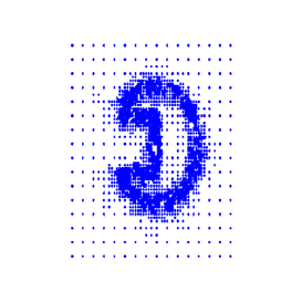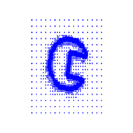
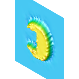
Figure 2 represents the evolution of the rotating cylinder on a half turn with a coarse mesh of $16\times 16$ points and 4 adaptive refinement levels. We notice that the cylinder is well represented and that the mesh points concentrate along the discontinuities.

4.2 The two-stream instability

We consider two streams symmetric with respect to $v=0$ and represented by the initial distribution function

$$f(0,x,v)=\frac{1}{\sqrt{2\pi}}v^{2}\,\exp(-v^{2}/2)(1+\alpha\,\cos(k_{0}\,x)),$$

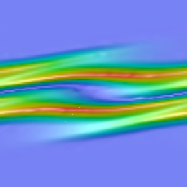
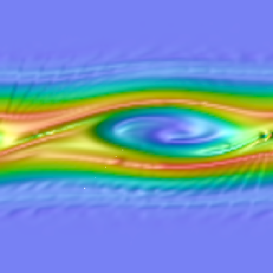
with $\alpha=0.25$, $k_{0}=0.5$, and $L=2\,\pi/k_{0}$. We use a maximum of $N_{x}=128$ points in the $x$ direction, and $N_{v}=128$ points in the $v$ direction with $v_{max}=7$, and a time step $\Delta t=1/8$. The solution varies first very slowly and then fine scales are generated. Between times of around $t\simeq 20\,\,\omega_{p}^{-1}$ and $t\simeq 40\,\,\omega_{p}^{-1}$, the instability increases rapidly and a hole appears in the middle of the computational domain. After $t=45\,\,\omega_{p}^{-1}$ until the end of the simulation, particles inside the hole are trapped. On figure 3 we show a snapshot of the distribution function at times $t=5\,\,\omega_{p}^{-1}$ and $t=30\,\,\omega_{p}^{-1}$ for a coarse mesh of $16\times 16$ points and 3 levels of refinement. The adaptive method reproduces well the results obtained in the non adaptive case.

Figure 3: Two stream instability for a coarse mesh of $2^{4}\times 2^{4}$, and 3 adaptive refinement levels, (left) at time $t=5\omega_{p}^{-1}$, (right) at time $t=30\omega_{p}^{-1}$.

5 Conclusion

In this paper we have described a new method for the numerical resolution of the Vlasov equation using an adaptive mesh of phase-space. The adaptive algorithm is based on a multiresolution analysis. It performs qualitatively well. However, there is a large overhead due to the handling of the adaptive mesh which has not been optimized yet. The performance of the code needs to be improved before we can recommend this technique for actual computations. We are currently working on optimizing the code and trying different kinds of wavelets, as well as obtaining error estimates for the adaptive method.

References

- (1) S. Bertoluzza, An adaptive collocation method based on interpolating wavelets. Multiscale wavelet methods for partial differential equations, pp. 109–135, Wavelet Anal. Appl., 6, Academic Press, San Diego, CA, 1997.
- (2) C.Z. Cheng, G. Knorr, The integration of the Vlasov equation in configuration space. J. Comput. Phys., 22 (1976), pp. 330–348.
- (3) A. Cohen, S.M. Kaber, S. Mueller and M. Postel, Fully adaptive multiresolution finite volume schemes for conservation laws, to appear in Mathematics of Computation.
- (4) M.R. Feix, P. Bertrand, A. Ghizzo, Eulerian codes for the Vlasov equation, Series on Advances in Mathematics for Applied Sciences, 22, Kinetic Theory and Computing (1994), pp. 45–81.
- (5) F. Filbet, E. Sonnendrücker, Numerical methods for the Vlasov equation, these proceedings.
- (6) A. Ghizzo, P. Bertrand, M. Shoucri, T.W. Johnston, E. Filjakow, M.R. Feix, A Vlasov code for the numerical simulation of stimulated Raman scattering, J. Comput. Phys., 90 (1990), no. 2, pp. 431–457.
- (7) M. Griebel, F. Koster, Adaptive wavelet solvers for the unsteady incompressible Navier-Stokes equations, Advances in Mathematical Fluid Mechanics J. Malek and J. Necas and M. Rokyta eds., Springer Verlag, (2000).
- (8) E. Sonnendrücker, J. Roche, P. Bertrand, A. Ghizzo, The Semi-Lagrangian Method for the Numerical Resolution of Vlasov Equations, J. Comput. Phys., 149 (1999), no. 2, pp. 201–220.
- (9) E. Sonnendrücker, J.J. Barnard, A. Friedman, D.P. Grote, S.M. Lund, Simulation of heavy ion beams with a semi-Lagrangian Vlasov solver, Nuclear Instruments and Methods in Physics Research, Section A, 464, no. 1-3, (2001), pp. 653–661.
- (10) S.T. Zalesak, Fully multidimensional flux-corrected transport algorithms for fluids, J. Comput. Phys., 31 (1979), no. 3, pp. 335–362.