Use of Triangular Elements for Nearly Exact BEM Solutions

Abstract

A library of C functions yielding exact solutions of potential and flux influences due to uniform surface distribution of singularities on flat triangular and rectangular elements has been developed. This library, ISLES, has been used to develop the neBEM solver that is both precise and fast in solving a wide range of problems of scientific and technological interest. Here we present the exact expressions proposed for computing the influence of uniform singularity distributions on triangular elements and illustrate their accuracy. We also present a study concerning the time taken to evaluate these long and complicated expressions vis a vis that spent in carrying out simple quadratures. Finally, we solve a classic benchmark problem in electrostatics, namely, estimation of the capacitance of a unit square plate raised to unit volt. For this problem, we present the estimated values of capacitance and compare them successfully with some of the most accurate results available in the literature. In addition, we present the variation of the charge density close to the corner of the plate for various degrees of discretization. The variations are found to be smooth and converging. This is in clear contrast to the criticism commonly leveled against usual BEM solvers.

Keywords: Boundary element method, triangular element, potential, flux, unit square plate, charge density, capacitance.

1 Introduction

One of the elegant methods for solving the Laplace / Poisson equations (normally an integral expression of the inverse square law) is to set up the Boundary Integral Equations (BIE) which lead to the moderately popular Boundary Element Method (BEM). In the forward version of the BEM, surfaces of a given geometry are replaced by a distribution of point singularities such as source / dipole of unknown strengths. The strengths of these singularities are obtained through the satisfaction of a given set of boundary conditions that can be Dirichlet, Neumann or of the Robin type. The numerical implementation requires considerable care [1] because it involves evaluation of singular (weak, strong and hyper) integrals. Some of the notable two-dimensional and three-dimensional approaches are [1] and [2, 3, 4, 5, 6] and the references in these papers. Despite a large body of literature, closed form analytic expressions for computing the effects of distributed singularities are rare [7, 8] and complicated to implement. Thus, for solving difficult but realistic problems involving, for example, sharp edges and corners or thin elements, introduction of complicated mathematics and special formulations becomes a necessity [9, 10]. These drawbacks are some of the major reasons behind the relative unpopularity of the BEM despite its significant advantages over domain approaches such as the finite-difference and finite-element methods (FDM and FEM) while solving non-dissipative problems [11]. It is well-understood that most of the difficulties in the available BEM solvers stem from the assumption of nodal concentration of singularities which leads to various mathematical difficulties and to the infamous numerical boundary layers [9, 12]. The Inverse Square Law Exact Solutions (ISLES) library, in contrast, is capable of truly modeling the effect of distributed singularities precisely and, thus, its application is not limited by the proximity of other singular surfaces or their curvature or their size and aspect ratio. The library consists of exact solutions for both potential and flux due to uniform distribution of singularity on flat rectangular and triangular elements. While the rectangular element can be of any arbitrary size [13, 14], the triangular element can be a right angled triangle of arbitrary size [15]. Since any real geometry can be represented through elements of the above two types (or by the triangular type alone), this library can help in developing solvers capable of solving three-dimensional potential problems for any geometry. It may be noted here that any non-right-angled triangle can be easily decomposed in to two right-angled triangles. Thus, the right-angled triangles considered here, in fact, can take care of any three-dimensional geometry. Several difficulties were faced in developing the library which arose due to the various terms of the integrals and also from the approximate nature of computation in digital computers. In this paper, we have discussed these difficulties, solutions adopted at present and possible ways of future improvement.

The classic benchmark problem of estimating the capacitance of a unit square plate raised to unit volt has been addressed using a solver based on ISLES, namely, the nearly exact BEM (neBEM) solver. Results obtained using neBEM have been compared with other precise results available in the literature. The comparison clearly indicates the excellent precision and efficiency achievable using ISLES and neBEM. In addition, we have also presented the variation of charge density close to the corner of the square plate. Usually, using BEM, it is difficult to obtain physically consistent results close to these geometric singularities. Wild variations in the magnitude of the charge density has been observed with the change in the degree of discretization, the reason once again being associated with the nodal model of singularities [16]. In contrast, using neBEM, we have obtained very smooth variation close to the corner. Moreover, the magnitudes of the charge density have been found to be consistently converging to physically realistic values. These results clearly indicate that since the foundation expressions of the solver are exact, it is possible to find the potential and flux accurately in the complete physical domain, including the critical near-field domain using neBEM. In addition, since singularities are no longer assumed to be nodal and we have the exact expressions for potential and flux throughout the physical domain, the boundary conditions no longer need to be satisfied at special points such as the centroid of an element. Although consequences of this considerable advantage is still under study, it is expected that this feature will allow neBEM to yield accurate estimates for problems involving corners and edges that are very important in a large number of scientific and technological studies.

It should be noted here that the exact expressions for triangular elements consist of a significantly larger number of mathematical operations than those for rectangular elements. Thus, for the solver, it is more economical if we use a mixed mesh of rectangular and triangular elements using rectangular elements as much as possible. However, in the present work, we have intentionally concentrated on the performance of the triangular elements and results shown here are those obtained using only triangular elements.

2 Exact Solutions

The expressions for potential and flux at a point $(X,Y,Z)$ in free space due to uniform source distributed on a rectangular flat surface having corners situated at $(x_{1},z_{1})$ and $(x_{2},z_{2})$ has been presented, validated and used in [13, 14] and, thus, is not being repeated here.

Here, we present the exact expressions necessary to compute the potential and flux due to a right-angled triangular element of arbitrary size, as shown in Fig.1. It may be noted here that the length in the X direction has been normalized, while that in the Z direction has been allowed to be of any arbitrary magnitude, $z_{M}$. From the figure, it is easy to see that in order to find out the influence due to triangular element, we have imposed another restriction, namely, the necessity that the X and Z axes coincide with the perpendicular sides of the right-angled triangle. Both these restrictions are trivial and can be taken care of by carrying out suitable scaling and appropriate vector transformations. It may be noted here that closed-form expressions for the influence of rectangular and triangular elements having uniform singularity distributions have been previously presented in [7, 8]. However, in these works, the expressions presented are quite complicated and difficult to implement. In [13] and in the present work, the expressions we have presented are lengthy, but completely straight-forward. As a result, the implementation issues of the present expressions, in terms of the development of the ISLES library and the neBEM solver are managed quite easily.

Figure 1: Right-angled triangular element with x-length 1 and an arbitrary z-length, $z_{M}$; P is the point where the influence (potential and flux) is being computed

It is easy to show that the influence (potential) at a point $P(X,Y,Z)$ due to uniform source distributed on a right-angled triangular element as depicted in Fig.1 can be represented as a multiple of

$$\phi(X,Y,Z)=\int_{0}^{1}\int_{0}^{z(x)}\frac{dx\,dz}{\sqrt{(X-x)^{2}+Y^{2}+(Z-z)^{2}}}$$ (1)

in which we have assumed that $x_{1}=0$, $z_{1}=0$, $x_{2}=1$ and $z_{2}=z_{M}$, as shown in the geometry of the triangular element. The closed-form expression for the potential has been obtained using symbolic integration [17] which was subsequently simplified through substantial effort. It is found to be significantly more complicated in comparison to the expression for rectangular elements presented in [13] and can be written as

$$\Phi=$$ (2)

$$\frac{1}{2}\left(\right.(z_{M}Y^{2}-XG)(LP_{1}+LM_{1}-LP_{2}-LM_{2})+i\left|Y\right|(z_{M}X+G)(LP_{1}-LM_{1}-LP_{2}+LM_{2})$$

$$-S_{1}X(tanh^{-1}(\frac{R_{1}+iI_{1}}{D_{11}|Z|})+tanh^{-1}(\frac{R_{1}-iI_{1}}{D_{11}|Z|})-tanh^{-1}(\frac{R_{1}+iI_{2}}{D_{21}|Z|})-tanh^{-1}(\frac{R_{1}-iI_{2}}{D_{21}|Z|}))$$

$$+iS_{1}|Y|(tanh^{-1}(\frac{R_{1}+iI_{1}}{D_{11}|Z|})-tanh^{-1}(\frac{R_{1}-iI_{1}}{D_{11}|Z|})-tanh^{-1}(\frac{R_{1}+iI_{2}}{D_{21}|Z|})+tanh^{-1}(\frac{R_{1}-iI_{2}}{D_{21}|Z|}))$$

$$+\frac{2G}{\sqrt{1+{z_{M}}^{2}}}\log\left(\right.\frac{\sqrt{1+{z_{M}}^{2}}D_{12}-E_{1}}{\sqrt{1+{z_{M}}^{2}}D_{21}-E_{2}}\left.\right)+2Z\log\left(\frac{D_{21}-X+1}{D_{11}-X}\right)\left.\right)+C$$

where,

$$D_{11}=\sqrt{(X-x_{1})^{2}+Y^{2}+(Z-z_{1})^{2}};\,D_{12}=\sqrt{(X-x_{1})^{2}+Y^{2}+(Z-z_{2})^{2}}$$

$$D_{21}=\sqrt{(X-x_{2})^{2}+Y^{2}+(Z-z_{1})^{2}};\,I_{1}=(X-x_{1})\,\left|Y\right|;\,I_{2}=(X-x_{2})\,\left|Y\right|$$

$$S_{1}={\it sign}(z_{1}-Z);\,R_{1}=Y^{2}+(Z-z_{1})^{2}$$

$$E_{1}=(X+{z_{M}}^{2}-z_{M}Z);\,E_{2}=(X-1-z_{M}Z),\,$$

$$G=z_{M}(X-1)+Z;\,H_{1}=Y^{2}+G(Z-z_{M});\,H_{2}=Y^{2}+GZ$$

$$LP_{1}=\frac{1}{G-iz_{M}|Y|}log(\frac{(H_{1}\,+GD_{12})+i|Y|(E_{1}-iz_{M}D_{12})}{-X+i|Y|})$$

$$LM_{1}=\frac{1}{G+iz_{M}|Y|}log(\frac{(H_{1}\,+GD_{12})-i|Y|(E_{1}-iz_{M}D_{12})}{-X-i|Y|})$$

$$LP_{2}=\frac{1}{G-iz_{M}|Y|}log(\frac{(H_{2}\,+GD_{21})+i|Y|(E_{2}-iz_{M}D_{21})}{1-X+i|Y|})$$

$$LM_{2}=\frac{1}{G+iz_{M}|Y|}log(\frac{(H_{2}\,+GD_{21})-i|Y|(E_{2}-iz_{M}D_{21})}{1-X-i|Y|})$$

and $C$ denotes a constant of integration.

Similarly, the flux components due to the above singularity distribution can also be represented through closed-form expressions as shown below:

$$F_{x}=-\frac{\partial\Phi}{\partial x}=$$ (3)

$$\frac{1}{2}\left(\right.(G)(LP_{1}+LM_{1}-LP_{2}-LM_{2})-i\left|Y\right|(z_{M})(LP_{1}-LM_{1}-LP_{2}+LM_{2})$$

$$+S_{1}(tanh^{-1}(\frac{R_{1}+iI_{1}}{D_{11}|Z|})+tanh^{-1}(\frac{R_{1}-iI_{1}}{D_{11}|Z|})-tanh^{-1}(\frac{R_{1}+iI_{2}}{D_{21}|Z|})-tanh^{-1}(\frac{R_{1}-iI_{2}}{D_{21}|Z|}))$$

$$+\frac{2z_{M}}{\sqrt{1+{z_{M}}^{2}}}\log\left(\right.\frac{\sqrt{1+{z_{M}}^{2}}D_{12}-E_{1}}{\sqrt{1+{z_{M}}^{2}}D_{21}-E_{2}}\left.\right)\left.\right)+C$$

$$F_{y}=-\frac{\partial\Phi}{\partial y}=$$

$$\frac{-1}{2}\left(\right.(2z_{M}Y)(LP_{1}+LM_{1}-LP_{2}-LM_{2})+i\left|Y\right|(Sn(Y)G)(LP_{1}-LM_{1}-LP_{2}+LM_{2})$$

$$+iS_{1}Sn(Y)(tanh^{-1}(\frac{R_{1}+iI_{1}}{D_{11}|Z|})-tanh^{-1}(\frac{R_{1}-iI_{1}}{D_{11}|Z|})-tanh^{-1}(\frac{R_{1}+iI_{2}}{D_{21}|Z|})+tanh^{-1}(\frac{R_{1}-iI_{2}}{D_{21}|Z|}))\left.\right)+C$$

and,

$$F_{z}=-\frac{\partial\Phi}{\partial z}=\left(\right.\frac{1}{\sqrt{1+{z_{M}}^{2}}}\log\left(\right.\frac{\sqrt{1+{z_{M}}^{2}}D_{21}-E_{2}}{\sqrt{1+{z_{M}}^{2}}D_{12}-E_{1}}\left.\right)+\log\left(\frac{D_{11}-X}{D_{21}-X+1}\right)\left.\right)+C$$ (5)

where $Sn(Y)$ implies the sign of the Y-coordinate and $C$ indicates constants of integrations. It is to be noted that the constants of different integrations are not the same. These expression are expected to be useful in the mathematical modeling of physical processes governed by the inverse square laws. Being exact and valid throughout the physical domain, they can be used to formulate versatile solvers to solve multi-scale multi-physics problems governed by the Laplace / Poisson equations involving Dirichlet, Neumann or Robin boundary conditions.

3 Development of the ISLES library

Due to the tremendous popularity of the C language we have written the codes in the C programming language. However, it should be quite simple to translate the library to other popular languages such as FORTRAN or C++, since no special feature of the C language has been used to develop the codes.

3.1 Validation of the exact expressions

The expressions for the rectangular element have been validated in detail in [13]. Here, we present the results for triangular elements in fair detail. In Fig.2, we have presented a comparison of potentials evaluated for a unit triangular element by using the exact expressions, as well as by using numerical quadrature of high accuracy. The two results are found to compare very well throughout. Please note that contours have been obtained on the plane of the element, and thus, represents a rather critical situation. Similarly, Fig.3 shows a comparison between the results obtained using closed-form expressions for flux and those obtained using numerical quadrature. The flux considered here is in the $Y$ direction and is along a line beginning from $(-2,-2,-2)$ and ending at $(2,2,2)$. The comparison shows the commendable accuracy expected from closed form expressions. In Fig.4(a) and 4(b), the surface plots of potential on the element plane ($XZ$ plane) and $Y$-flux on the $XY$ plane have been presented from which the expected significant increase in potential and sharp change in the flux value on the element is observed. Thus, by using a small fraction of computational resources in comparison to those consumed in numerical quadratures, ISLES can compute the exact value of potential and flux for singularities distributed on triangular elements.

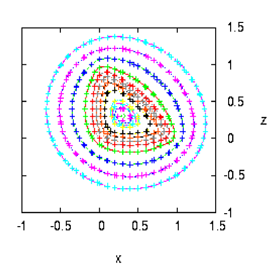
Figure 2: Potential contours on a triangular element computed using exact expressions and by numerical quadrature

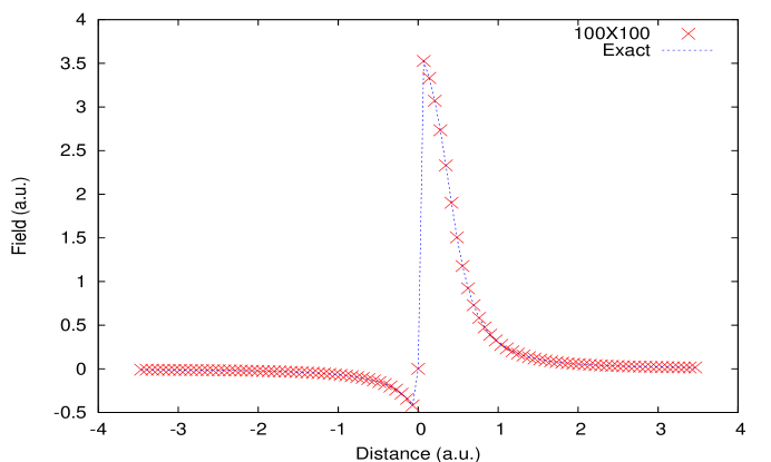
Figure 3: Comparison of flux (in the Y direction) as computed by ISLES and numerical quadrature along a diagonal line

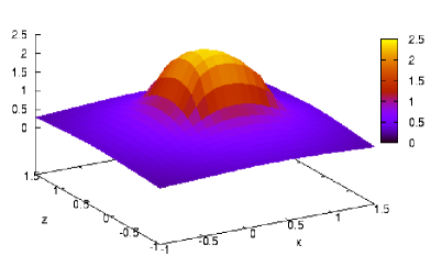
(a) Potential surface

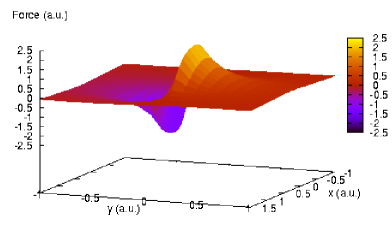
(b) Flux surface

Figure 4: (a) Potential surface due to a triangular source distribution on the element plane, (b) Flux (in the Y direction) surface due to a triangular source distribution on the XY plane at Z=0

3.2 Near-field performance

In order to emphasize the accuracy of ISLES, we have considered the following severe situations in the near-field region in which it is observed that the quadratures can match the accuracy of ISLES only when a high degree of discretization is used. Please note that in these cases, the value of $z_{M}$ has been considered to be 10. In Fig.5 we have presented the variation of potential along a line on the element surface running parallel to the Z-axis of the triangular element (see Fig.1) and going through the centroid of the element. It is observed that results obtained using even a $100\times 100$ quadrature is quite unacceptable. In fact, by zooming on to the image, it can be found that only the maximum discretization yields results that match closely to the exact solution. It may be noted here that the potential is a relatively easier property to compute. The difficulty of achieving accurate flux estimates is illustrated in the two following figures. The variation of flux in the $X$-direction along the same line as used in Fig.5 has been presented in Fig.6. Similarly, variation of $Y$-flux along a diagonal line (beginning at (-10,-10,-10) and ending at (10,10,10) and piercing the element at the centroid) has been presented in Fig.7. From these figures we see that the flux values obtained using the quadrature are always inaccurate even if the discretization is as high as $100\times 100$. We also observe that the estimates are locally inaccurate despite the use of very high amount of discretization ($200\times 200$ or $500$). Specifically, in the latter figure, even the highest discretization can not match the exact values at the peak, while in the former only the highest one can correctly emulate the sharp change in the flux value. It is also heartening to note that the values from the quadrature using higher amount of discretization consistently converge towards the ISLES values.

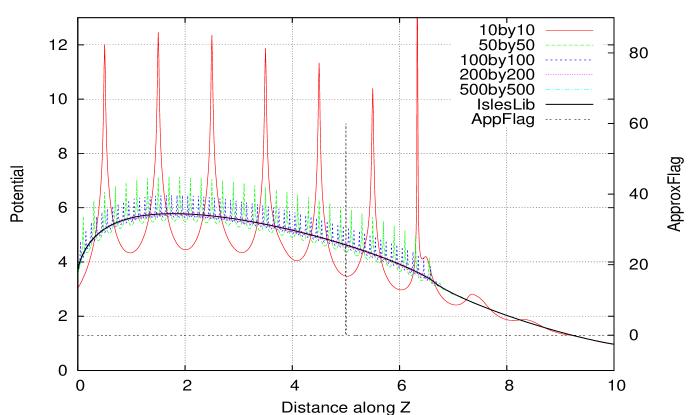
Figure 5: Variation of potential along a centroidal line on the XZ plane parallel to the Z axis for a triangular element: comparison among values obtained using the exact expressions and numerical quadratures

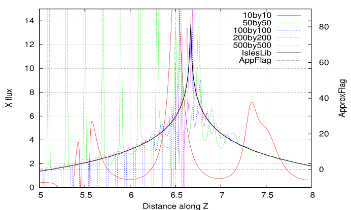
Figure 6: Variation of flux in the X direction along a line on the XZ plane parallel to the Z axis for a triangular element: comparison among values obtained using the exact expressions and numerical quadratures

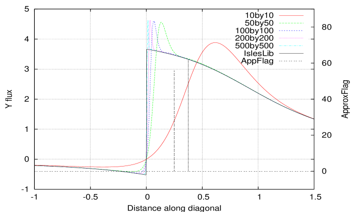
Figure 7: Comparison of flux (in the Y direction) along a diagonal line piercing the triangular element at the centroid: comparison among values obtained using the exact expressions and numerical quadratures

3.3 Far field performance

It is expected that beyond a certain distance, the effect of the singularity distribution can be considered to be the same as that of a centroidally concentrated singularity or a simple quadrature. The optimized amount of discretization to be used for the quadrature can be determined from a study of the speed of execution of each of the functions in the library and has been presented separately in a following sub-section. If we plan to replace the exact expressions by quadratures (in order to reduce the computational expenses, presumably) beyond a certain given distance, the quadrature should necessarily be efficient enough to justify the replacement. While standard but more elaborate algorithms similar to the fast multipole method (FMM) [18] along with the GMRES [19] matrix solver can lead to further of computational efficiency, the simple approach as outlined above can help in reducing a fair amount of computational effort. In the following, we present the results of numerical experiments that help us in determining the far-field performance of the exact expressions and quadratures of various degrees that, in turn, help us in choosing the more efficient approach for a desired level of accuracy.

In Fig.8 we have presented potential values obtained using the exact approach, $100\times 100$, $10\times 10$ and no discretization, i.e., the usual BEM approximation while using the zeroth order piecewise uniform charge density assumption. The potentials are computed along a diagonal line running from (-1000, -1000, -1000) to (1000, 1000, 1000) which pierces a triangular element of $z_{M}=10$. It can be seen that results obtained using the usual BEM approach yields inaccurate results as we move closer than distances of 10 units, while the $10\times 10$ discretization yields acceptable results up to a distance of 1.0 unit. In order to visualize the errors incurred due to the use of quadratures, we have plotted Fig.9 where the errors incurred (normalized with respect to the exact value) have been plotted. From this figure we can conclude that for the given diagonal line, the error due to the usual BEM approximation falls below 1% if the distance is larger than 20 units while for the simple $10\times 10$ discretization, it is 2 units. It may be mentioned here that along the axes the error turns out to be significantly more [13] and the limits need to be effectively doubled to achieve the accuracy for all cases possible. Thus, for achieving 1% accuracy, the usual BEM is satisfactory only if the distance of the influenced point is five times the longer side of an element. Please note here that the error drops to 1 out of $10^{6}$ as the distance becomes fifty times the longer side. Besides proving that the exact expressions work equally well in the near-field as well as the far-field, this fact justifies the usual BEM approach for much of the computational domain leading to substantial savings in computational expenses.

Figure 8: Potential along a diagonal through the triangular element computed using exact, $100\times 100$, $10\times 10$ and usual BEM approach

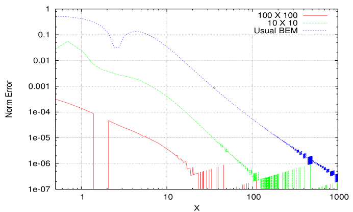
Figure 9: Error along a diagonal through the triangular element computed using $100\times 100$, $10\times 10$ and usual BEM approach

The accuracy of the exact expressions used in the ISLES library is confirmed from the above comparisons. However, there are several other important issues related to the development of the library that are discussed below briefly.

3.4 Evaluation of the component functions

Many of the irrational and transcendental functions have domains and ranges in which they are defined. Moreover, they are often multiply defined in the complex domain; for example, there are an infinite number of complex values for the logarithm function. In such cases, only one principal value must be returned by the function. In general, such values cannot be chosen so as to make the range continuous and thus, lines in the domain called branch cuts need to be defined, which in turn define the discontinuities in the range. While evaluating expressions such as the ones displayed in eqns.(2 - 5) a number of such problems are expected to occur. However, when the expressions are analyzed at critical locations such as the corners and edges of the element, it is observed that the terms likely to create difficulties while evaluating potentials are either cancelled out or are themselves multiplied by zero. As a result, at these locations of likely geometric and mathematical singularities, the solution behaves nicely. However, the same is not true for the expressions related to the flux components. For these, we have to deal with branch-cut problems in relation to $tanh^{-1}$ and problems related to the evaluation of $log(0)$. It should be noted here that these singularities associated to the edges and corners of the elements are of the weak type and it is expected that exact evaluation of these terms as well will be possible through further work.

However, difficulties of a different nature crop up in these calculations which can be linked directly to the limitation of the computer itself, namely, round-off errors [15]. These errors can lead to severe problems while handling multi-scale problems such as those described in [13]. A completely different approach is necessary to cope up with these difficulties, for example, the use of extended range arithmetic [20], interval arithmetic [21] or the use of specialized libraries such as the CORE library of the Exact Geometric Computation (EGC) initiative [22]. In the present version of ISLES, a simple approach has been implemented which sets a lower limit to various distance values. Below this value, the distance is considered to be zero. Plan of future improvements in this regard has been kept at a high priority.

3.4.1 Algorithm

As discussed above, there are possibilities of facing problems while using the exact expressions which may be due to the functions being evaluated or due to round-off errors leading to erroneous results. Moreover, despite providing many checks during the computation there is finite possibility of ending up with a wrong value of a property indicated by its being Nan or inf or potential due to unit positive singularity strength turning out to be negative. In order to maintain the robustness of the library, we have tried to keep checks on the intermediate and final values during the course of the computation. When the results are found to be unsatisfactory, unphysical, we have re-estimated the results by using numerical quadrature and kept a track of the cause by raising a unique approximation flag which is specific for a problem. As a result, the steps for the calculation for a property can be written as follows:

• Get the required inputs - geometry of the element and the position where the effect needs to be evaluated; Check whether the element size and distances are large enough so that the results do not suffer from round-off errors.

• Check whether the location coincides with one of the special ones, such as corners or edges.

• Evaluate the necessary expressions in accordance with the foregoing results. If necessary, consider each term in the expressions separately to sort out difficulties related to singularities, branch-cuts or round-off errors. Note that if the multiplier is zero, rest of the term does not need evaluation.

• If direct evaluation of the expressions fail, raise a unique approximation flag specific to this problem and term and return the value of the property by using numerical quadrature.

• Compute all the terms and find the final value, Check whether the final value is a number and physically meaningful. If not satisfied, recompute the result using numerical quadrature and raise the relevant approximation flag.

3.5 Speed of execution

The time taken to compute the potential and flux is an important parameter related to the overall computational efficiency of the codes. This is true despite the fact that, in a typical simulation, the time taken to solve the system of algebraic equation is far greater than the time taken to build the influence coefficient matrix and post-processing. Moreover, the amount of time taken to solve the system of equations tend to increase at a greater rate than the time taken to complete the other two. It should be mentioned here that the time taken in each of these steps can vary to a significant amount depending on the algorithm of the solver. In the present case, the system of equations has been solved using lower upper decomposition using the well known Crout’s partial pivoting. Although this method is known to be very rugged and accurate, it is not efficient as far as number of arithmetic operations, and thus, time is concerned. It is also possible to reduce the time taken to pre-process (generation of mesh and creation of influence matrices), solve the system of algebraic equations and that for post-process (computation of potential and flux at the required locations) can be significantly reduced by adopting faster algorithms, including those involving parallelization.

In order to optimize the time taken to generate the influence coefficient matrix and that to carry out the post-processing, we carried out a small numerical study to determine the amount of time taken to complete the various functions being used in ISLES, especially those being used to evaluate the exact expressions and those being used to carry out the quadratures. The results of the study (which was carried out using the linux system command gprof) has been presented in the following Table1.

Table 1: Time taken to evaluate exact expression and various quadratures

Method	Exact	Usual BEM	$10\times 10$	$100\times 100$	$500\times 500$
Time	0.8 $\mu s$	25 $ns$	1 $\mu s$	200 $\mu s$	5 $ms$

Please note that the numbers presented in this table are representative and are likely to have statistical fluctuations. However, despite the fluctuations, it may be safely concluded that a quadrature having only $10\times 10$ discretization is already consuming time that is comparable to that needed exact evaluation. Thus, the exact expressions, despite their complexity, are extremely efficient in the near-field which can be considered at least as large as 0.5 times the larger side of a triangular element (please refer to Fig.9). In making this statement, we have assumed that the required accuracy for generating the influence coefficient matrix and subsequent potential and flux calculations is 1%. This may not be acceptable at all under many practical circumstances, in which case the near-field would imply a larger volume.

3.6 Salient features of ISLES

Development of usual BEM solvers are dependent on the two following assumptions:

• While computing the influences of the singularities, the singularities are modeled by a sum of known basis functions with constant unknown coefficients. For example, in the constant element approach, the singularities are assumed to be concentrated at the centroid of the element, except for special cases such as self influence. This becomes necessary because closed form expressions for the influences are not, in general, available for surface elements. An approximate and computationally rather expensive way of circumventing this limitation is to use numerical integration over each element or to use linear or higher order basis functions.

• The strengths of the singularities are solved depending upon the boundary conditions, which, in turn, are modeled by the shape functions. For example, in the constant element approach, it is assumed that it is sufficient to satisfy the boundary conditions at the centroids of the elements. In this approach, the position of the singularity and the point where the boundary condition is satisfied for a given element usually matches and is called the collocation point.

The first (and possibly, the more damaging) approximation for BEM solvers can be relaxed by using ISLES and can be restated as,

• The singularities distributed on the boundary elements are assumed to be uniform on a particular element. The strength of the singularity may change from element to element.

This improvement turns out to be very significant as demonstrated in the following section and some of our other studies involving microelectromechanical systems (MEMS) and gas detectors for nuclear applications [13, 14]. Some of the advantages of using ISLES are itemized below:

• For a given level of discretization, the estimates are more accurate,

• Effective efficiency of the solver improves, as a result,

• Large variation of length-scales, aspect ratios can be tackled,

• Thinness of members or nearness of surfaces does not pose any problem,

• Curvature has no detrimental effect on the solution,

• The boundary condition can be satisfied anywhere on the elements, i.e., points other than the centroidal points can be easily used, if necessary (for a corner problem, may be),

• The same formulation, library and solver is expected to work in majority of physical situations. As a result, the necessity for specialized formulations of BEM can be greatly minimized.

4 Capacitance of a unit square plate - a classic benchmark problem

Using the neBEM solver, we have computed the capacitance of a unit square conducting plate raised to a unit volt. This problem is still considered to be one of the major unsolved problems of electrostatic theory [23, 8, 26, 16] and no analytical solution for this problem has been obtained so far. The capacitance value estimated by the present method has been compared with very accurate results available in the literature (using BEM and other methods). The results obtained using the neBEM solver is found to be among the most accurate ones available till date as shown in Table.2. Please note that we have not invoked symmetry or used extrapolation techniques to arrive at our result presented in the table.

Table 2: Comparison of capacitance values

Reference	Method	Capacitance (pF) / 4 $\pi\epsilon_{0}$
[23]	Surface Charge	0.3607
[24]	Surface Charge	0.362
[25]	Surface Charge	0.367
[8]	Refined Surface Charge	$0.3667892\pm 1.1\times 10^{-6}$
	and Extrapolation
[26]	Refined Boundary Element	$0.3667874\pm 1\times 10^{-7}$
	and Extrapolation
[27]	Numerical Path Integration	$0.36684$
[16]	Random Walk	$0.36\pm 0.01$
This work	neBEM	0.3660587

Finally, we consider the corner problem related to the electrostatics of the above conducting plate. Problems of this nature are considered to be challenging for any numerical tool and especially so for the BEM approach. The inadequacy of the BEM approach, especially in solving the present problem, has been mentioned even quite recently [16] in which it has been correctly mentioned that since the method can not extend its mathematical model to include the edges and corners in reality, it is unlikely that it will ever succeed in modeling the edge / corner singularities correctly. As a result, with change in discretization, the properties near these geometric singularities are expected to oscillate significantly leading to erroneous results. However, as discussed above, the neBEM does extend its singularities distributed on the surface elements right till an edge or a corner. Moreover, using neBEM, it is also possible to satisfy the boundary conditions (both potential and flux) as close to the edge / corner as is required. In fact, it should be possible to specify the potentials right at the edge / corner.

In the following study, we have presented estimates of charge density very close the flat plate corner as obtained using neBEM. Please note that the boundary conditions have been satisfied at the centroids of each element although we plan to carry out detailed studies of changing the position of these points, especially in relation to problems involving edges / corners. In Fig.10, charge densities very close to the corner of the flat plate estimated by neBEM using various amounts of discretization have been presented. It can be seen that each curve follows the same general trend, does not suffer from any oscillation and seems to be converging to a single curve. This is true despite the fact that there has been almost an order of magnitude variation in the element lengths.

Finally, in Fig.11, we present a least-square fitted straight line matching the charge density as obtained the highest discretization in this study. It is found that the slope of the straight line is 0.713567, which compares very well with both old and recent estimates of 0.7034 [28, 29]. This is despite the fact that here we have used a relatively coarse discretization near the corner. It should be mentioned that none of the earlier references cited here used the BEM approach. While the former used a singular perturbation technique, the latter used a diffusion based Monte-Carlo method. Thus, it is extremely encouraging to note that using the neBEM approach, we have been able to match the accuracy of these sophisticated techniques.

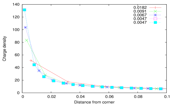
Figure 10: Corner charge density estimated by neBEM using various sizes of triangular elements

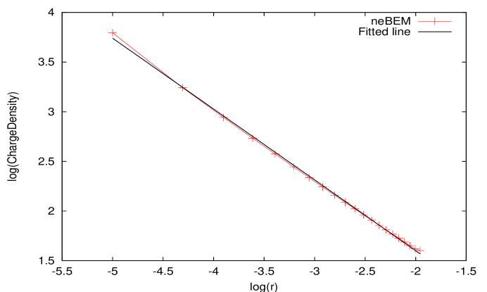
Figure 11: Variation of charge density with increasing distance from the corner of the unit square plate and a least-square fitted straight line: slope of the fitted line is 0.713567

5 Conclusion

An efficient and robust library for solving potential problems in a large variety of science and engineering problems has been developed. Exact closed-form expressions used to develop ISLES have been validated throughout the physical domain (including the critical near-field region) by comparing these results with results obtained using numerical quadrature of high accuracy. Algorithmic aspects of this development have also been touched upon. A classic benchmark problem of electrostatics has been successfully simulated to very high precision. Charge density values at critical geometric locations like corners have been found to be numerically stable and physically acceptable. Several advantages over usual BEM solvers and other specialized BEM solvers have been briefly mentioned. Work is under way to make the code more robust and efficient through the implementation of more efficient algorithms and parallelization.

Acknowledgements
We would like to thank Professor Bikas Sinha, Director, SINP and Professor Sudeb Bhattacharya, Head, INO Section, SINP for their support and encouragement during the course of this work.

References

- [1] Nagarajan, A., Mukherjee, S., 1993, “A mapping method for numerical evaluation of two-dimensional integrals with 1/r singularity”, Computational Mechanics, 12, pp.19-26.
- [2] Cruse, T.A., 1969, “Numerical solutions in three dimensional elastostatics”, (Int. J. Solids Struct., 5, pp.1259-1274.
- [3] Kutt, H.R., 1975, “The numerical evaluation of principal value integrals by finite-part integration”, Numer. Math., 24, pp.205-210.
- [4] Lachat, J.C., Watson, J.O., 1976, “Effective numerical treatment of boundary integral equations: A formulation for three dimensional elastostatics”, Int. J. Numer. Meth. Eng., 10, pp.991-1005.
- [5] Srivastava, R., Contractor, D.N., 1992, “Efficient evaluation of integrals in three-dimensional boundary element method using linear shape functions over plane triangular elements”, Appl. Math. Modelling, 16, pp.282-290.
- [6] Carini, A., Salvadori, A., 2002, “Analytical integration in 3D BEM: preliminaries”, Computational Mechanics, 18, pp.177-185.
- [7] Newman, J.N., 1986, “Distributions of sources and normal dipoles over a quadrilateral panel”, Jour. of Engg. Math., 20, pp.113-126.
- [8] Goto, E., Shi, Y. and Yoshida, N., 1992, “Extrapolated surface charge method for capacity calculation of polygons and polyhedra”, Jour. of Comput. Phys., 100, pp.105-115.
- [9] Chyuan, S-W., Liao, Y-S. and Chen, J-T., 2004, “An efficient technique for solving the arbitrarily multilayered electrostatic problems with singularity arising from a degenerate boundary”, Semicond. Sci. Technol., 19, R47-R58.
- [10] Bao, Z., Mukherjee, S., 2004, “Electrostatic BEM for MEMS with thin conducting plates and shells”, Eng Analysis Boun Elem, 28, pp.1427-1435.
- [11] Mukhopadhyay, S., Majumdar, N., 2006, “Effect of finite dimensions on the electric field configuration of cylindrical proportional counters”, IEEE Trans Nucl Sci, 53, pp.539-543.
- [12] Sladek, V., Sladek, J., 1991, “Elimination of the boundary layer effect in BEM computation of stresses”, Comm. Appl. Num. Meth., 7, pp.539-550.
- [13] Mukhopadhyay, S., Majumdar, N., 2006, “Computation of 3D MEMS electrostatics using a nearly exact BEM solver”, Eng Anal Boundary Elem, 30, pp.687-696.
- [14] Majumdar, N., Mukhopadhyay, S., 2006, “Simulation of three-dimensional electrostatic field configuration in wire chambers: A novel approach”, Nucl. Instrum. Meth. Phys. Res. A, 566, pp.489-494.
- [15] Mukhopadhyay, S., Majumdar, N., 2007, “Use of rectangular and triangular elements for nearly exact BEM solutions”, Emerging Mechanical Technology - Macro to Nano, Research Publishing Services, Chennai, India, pp.107-114 (ISBN: 81-904262-8-1).
- [16] Wintle, H.J., 2004, “The capacitance of the cube and square plate by random walk methods”, J Electrostatics, 62 pp.51-62.
- [17] Etter, D.M., 1997, Engineering Problem Solving with MatLab, Prentice Hall, International, Inc., New Jersey 07458, USA.
- [18] Greengard, L., Rokhlin, V., 1987, “A fast algorithm for particle simulation”, Journal of Computational Physics, 73 pp.325-348.
- [19] Saad, Y., Schultz, M., 1986, “GMRES: A generalized minimal residual algorithm for solving nonsymmetric linear systems”, SIAM J. Sci. Statist. Comput., 7 pp.856-869.
- [20] Smith, J.M., Olver, F.W., Lozier, D.W., 1981, “Extended-Range Arithmetic and Normalized Legendre Polynomial”, ACM Transactions on Mathematical Software, 7, pp.93-105.
- [21] Alefeld, G., Herzberger, J., 1983, Introduction to interval analysis, Academic Press.
- [22] http://cs.nyu.edu/exact/
- [23] Maxwell, J.C., 1878, Electrical Research of the Honorable Henry Cavendish, p.426, Cambridge University Press, Cambridge, UK.
- [24] Reitan, D.K., Higgins, R.J., 1957, “Accurate determination of capacitance of a thin rectangular plate”, Trans AIEE, Part 1, 75, pp.761-766.
- [25] Solomon, L., 1964, C.R.Acad.Sci III, 258, pp.64.
- [26] Read, F.H., 1997, “Improved extrapolation technique in the boundary element method to find the capacitance of the unit square and cube”, J Comput Phys, 133, pp.1-5.
- [27] Mansfield, M.L., Douglas, J.F., Garboczi, E.J., 2001, “Intrinsic viscosity and the electrical polarizability of arbitrarily shaped objects”, Phys Rev E, 64, 6, pp.061401-16.
- [28] Morrison, J.A., Lewis, J.A., 1975, “Charge singularity at the corner of a flat plate”, SIAM J. Appl. Math., 31, no. 2, pp.233-250.
- [29] Hwang, C-O., Won, T., 2005, “Last-passage algorithms for corner charge singularity of conductors”, Jour. Kor. Phys. Soc., 47, pp.S464-S466.