Green Function theory vs. Quantum Monte Carlo Calculation for thin magnetic films

Abstract

In this work we compare numerically exact Quantum Monte Carlo (QMC) calculations and Green function theory (GFT) calculations of thin ferromagnetic films including second order anisotropies. Thereby we concentrate on easy plane systems, i.e. systems for which the anisotropy favors a magnetization parallel to the film plane. We discuss these systems in perpendicular external field, i.e. $B$ parallel to the film normal. GFT results are in good agreement with QMC for high enough fields and temperatures. Below a critical field or a critical temperature no collinear stable magnetization exists in GFT. On the other hand QMC gives finite magnetization even below those critical values. This indicates that there occurs a transition from non-collinear to collinear configurations with increasing field or temperature. For slightly tilted external fields a rotation of magnetization from out-of-plane to in-plane orientation is found with decreasing temperature.

I Introduction

The fast development of technological applications based on magnetic systems in the last years, e.g. magnetic data storage devices, causes a high interest in thin magnetic films. One precondition for the technological development is the investigation of magnetic anisotropies and spin reorientation transitions connected therewith. Those reorientation transitions can occur from out-of-plane to in-plane or vice versa for increasing film thickness $d$farle , temperature $T$ wandlitz17 ; wandlitz18 ; wandlitz19 ; wandlitz20 ; wandlitz21 ; wandlitz22 ; wandlitz24 , or external field $B_{0}$.
Quantum Monte Carlo (QMC) calculations give the possibility to compare numerically exact results with analytical approximations. In Ref. qm, the authors investigated a ferromagnetic monolayer including positive second order anisotropy (easy axis perpendicular to the film plane). They discuss the temperature dependence of the magnetization $\langle S_{z}\rangle(T)$ as well as field induced reorientation transitions from out-of-plane to in-plane and compare the QMC results with Green function theory (GFT). They found good agreement in the case of applied external field in the easy direction (here $z$-axis). However, their GFT fails for external field applied in arbitrary direction, especially in the hard direction (within the film plane). As shown in Ref. schwieger1, for getting closer to the QMC results for magnetic field induced reorientation from out-of-plane to in-plane a more careful treatment of the local anisotropy terms is needed. In Refs. schwieger1, ; schwieger2, ; dipolpaper, ; pini, a decoupling scheme was presented which yields excellent agreement with QMC results for out-of-plane systems.
The availability of theories such as GFT and their check against state-of-the-art numerical algorithms is highly desirable because of the size limitations of systems where QMC can be performed. On the other hand the extension of GFT from a monolayer (where it can be compared to QMC as in the the present work) to multilayer systems is a straightforward task without further approximationsschwieger2 .
Up to now, to our knowledge, there is no comparison between QMC and approximative theories for easy-plane systems and it is not obvious that the theory presented in Refs. schwieger1, ; schwieger2, ; dipolpaper, ; pini, can reproduce the QMC results for in-plane systems as accurately as for the out-of-plane case. In contrast to the easy-axis case where a certain direction is preferred by the single ion anisotropy in easy-plane systems the full xy-plane is favored and no particular direction is distinguished within the plane. A magnetic field applied perpendicular to the plane does not destroy the $xy$-symmetry.
For systems exhibiting this kind of symmetry it was shown in a classical treatment that for external fields smaller than a critical field $0\leq B<B_{crit}$ ($B\>||\>z$) stable vortices, i.e. a non-collinear arrangement of spins, can existwysin98 ; vedmedenko99 ; lee04 ; rapini07 ; ivanov02 . These vortices can undergo a Berezinskii-Kosterlitz-Thouless (BKT) transitionkosterlitz73 . Depending on the strength of the anisotropy $K_{2}$ there might be vortices with or without a finite z-component of magnetizationwysin98 . In the small anisotropy case (which is considered in this work, $|K_{2}|<0.1J$) there is a finite out-of-plane component and for zero field the two possible directions of magnetization ($\pm z$) are energetically degenerate. For increasing magnetic field in z-direction the vortices antiparallel to the field become more and more unstable (heavy vortices). However the so called light vortices (parallel to the field) are stable up to a critical field $B_{z}=B_{crit}$ and contribute a finite $z$-component to the net-magnetization of the considered system ivanov02 .
The vortices in connection with a finite z-component of the net-magnetization emerge because of two reasons: first the competition between the anisotropy (favoring a orientation of the magnetization within the $xy$-plane) and the external field (favoring a perpendicular magnetization), and second: the $xy$-symmetry of the system, which does not allow for a rotated homogeneous phase.
In this paper we investigate both aspects, i.e. the field vs. anisotropy competition as well as the symmetry properties in detail for a quantum mechanical system. We will compare the results of QMC and GFT calculations.
As explained in more detail below, the QMC algorithm used here allows only for an external field applied in $z$-direction. Thus the $xy$-symmetry can not be broken and no comparison between $xy$-symmetric and asymmetric systems is possible. We will use GFT to clarify the influence of this symmetry breaking on the homogeneous phase. On the other hand, the GFT used here is by ansatz limited to the homogeneous phase. Therefore it can not describe a non-collinear (e.g, vortex-) magnetic phase, which is expected for $B\>||\>z$ and small field strengths. The breakdown of magnetization in GFT as well as an exposed maximum in the magnetization in QMC at certain critical values of the external field or temperature gives, however, a clear fingerprint of non-collinear configurations, at least if there is no meta-stable homogeneous phase. Below these critical values there will be a finite $z$-component in QMC and a vanishing magnetization in GFT.
For parameters, where both theories are applicable, QMC serves as a test for the approximations needed in GFT.

In this work we find indications for non-collinear spin configurations below a critical field or temperature for $B\>||\>z$ by comparing results of QMC and GFT as explained in the last clause. Above the critical field we obtain good agreement between QMC and GFT results. Breaking the $xy$-symmetry by adding a small $x$-component to the external field yields a stable collinear solution in GFT. The $z$-component of the magnetization in this case is in good agreement with the QMC results calculated with untilted field. Thus we can conclude that except for the restriction to collinear magnetic states GFT describes the competition between external field and anisotropy quite well.

The paper is organized as follows: First we explain the basics of the GFT and the QMC calculations. Then we apply both approaches to easy-plane systems in external magnetic fields and report the results of our calculations.

II Theory

II.1 Green Function Theory

In the following we present our theoretical approach using Green function theory. The focus of this work lies on the translational invariant system of a two-dimensional monolayer. Therefore the following Hamiltonian is used:

$$H = -\frac{1}{2}\sum_{ij}J_{ij}\mathbf{S}_{i}\mathbf{S}_{j}-\mathbf{B}\sum_{i}\mathbf{S}_{i}-K_{2}\sum_{i}(S_{z,i})^{2}.$$ (1)

The first term describes the Heisenberg coupling $J_{ij}$ between spins $\mathbf{S}_{i}$ and $\mathbf{S}_{j}$ located at sites $i$ and $j$. The second term contains an external magnetic field $\mathbf{B}$ in arbitrary direction (the Land$\rm\acute{e}$ factor $g_{J}$ and the Bohr magneton $\mu_{B}$ are absorbed in $\mathbf{B}$). The third term represents second order lattice anisotropy due to spin-orbit coupling. $S_{z,i}$ is the $z$-component of $\mathbf{S}_{i}$ (the $z$-axis of the coordinate system is oriented perpendicular to the film-plane). The lattice anisotropy favours in-plane ($K_{2}<0$) or out-of-plane ($K_{2}>0$) orientation. Our Hamiltonian is similar to that used in Refs. wandlitz, ; jensen2000, ; schwieger1, ; schwieger2, ; pini, for the investigation of the magnetic anisotropy and the field induced reorientation transition. To simplify calculations we consider nearest neighbor coupling only

$$J_{ij}=\left\{\begin{array}[]{cc}J&~{}~{}(i),(j)\text{ n.n.}\\ 0&\text{otherwise.}\end{array}\right.$$ (4)

The main idea of the special treatment presented in Refs. schwieger1, ; schwieger2, ; dipolpaper, ; pini, is that, before any decoupling is applied, the coordinate system $\Sigma$ is rotated to a new system $\Sigma^{\prime}$ where the new $z^{\prime}$-axis is parallel to the magnetization implying a collinear alignment of all spins within the layer. Then a combination of Random Phase approximation (RPA)RPA for the nonlocal terms in Eq. (1) (Heisenberg exchange interaction term) and Anderson-Callen approximation (AC)ac for the local lattice anisotropy term is applied in the rotated system. After application of the approximation one gets an effective anisotropy

$$K_{eff}(T)=2K_{2}\left(1-\frac{1}{2S^{2}}\left(S(S+1)-\langle S^{2}_{z\prime}\rangle\right)\right)\langle S_{z\prime}\rangle$$ (5)

where $\langle S_{z\prime}\rangle$ is the norm of the magnetization and $S$ is the spin quantum number, that we have chosen to be $S=1$ in all our calculations.
As shown in comparison with an exact treatment of the local anisotropy term in Ref. exakt, this approximation still holds up to anisotropy strengths $K_{2}\sim 1/2J$. Therefore we restrict ourselves in the following to small anisotropies ($K_{2}\leq 0.1J$) as found in most real materials. For a magnetic field applied in the $xz$-plane ($\mathbf{B}=(B_{x},0,B_{z})$) our theory gives a condition for the polar angle $\theta$ of the magnetization:

$$\sin\theta B_{z}-\cos\theta B_{x}+K_{eff}\sin\theta\cos\theta=0$$ (6)

The uniform magnon energies ($\mathbf{q}=\mathbf{0}$) which dominate the physical behavior of the magnetic system can easily be extracted from the theory dipolpaper ; pini :

$$E_{\mathbf{q}=\mathbf{0}}^{2}=\left(\cos\theta B_{z}+\sin\theta B_{x}+K_{eff}(\cos^{2}\theta-\sin^{2}\theta)\right)\cdot\\ \left(\cos\theta B_{z}+\sin\theta B_{x}+K_{eff}\cos^{2}\theta\right)$$ (7)

This result coincides with the spin-wave result pini if one replaces $\langle S_{z\prime}\rangle$ by the spin quantum number $S$ and $K_{eff}$ by the bare anisotropy constant $K_{2}$ in Eq. (7). For an easy-plane system ($K_{eff}<0$) with external field $B$ in $z$-direction the polar angle $\theta$ of the magnetization is given by:

$$\cos\theta=\left\{\begin{array}[]{cc}-B/K_{eff}(T)&~{}~{}\text{for}~{}~{}B<|K_{eff}(T)|\\ 1&\text{otherwise}\end{array}\right.$$ (10)

By inserting Eq.(10) into Eq.(7) one immediately gets:

$$E^{K_{eff}<0}_{\mathbf{q}=\mathbf{0}}(B)=\left\{\begin{array}[]{cc}0&B<|K_{eff}(T)|\\ B+K_{eff}(T)&\text{otherwise.}\end{array}\right.$$ (13)

For gapless magnon energies $E_{\mathbf{q}=\mathbf{0}}=0$ the magnon occupation number $\phi$ diverges ($\phi\rightarrow\infty$) in film systems with ferromagnetic coupling $J>0$ and the magnetization becomes zero $\langle S_{z\prime}\rangle=0$ in the collinear phase. This can be seen by following an argument of Blochbloch30 already given in 1930. Since the spin wave dispersion is $E\approx q^{2}$ in the vicinity of $\mathbf{q}=\mathbf{0}$ the spin-wave density of states $N(E)$ is independent of $E$ for a two-dimensional system for $E$ close to zero. The excitation of spin-waves at finite temperature leads to a variation of the magnetization of the order:

$$\Delta m(T) \sim \int_{0}^{\infty}\frac{N(E)dE}{\exp(E/k_{B}T)-1)}$$ (14)

$$\sim k_{B}T\int_{0}^{\infty}\frac{dx}{\exp(x)-1}.$$

Since the integral in Eq. (14) diverges for $T\neq 0$ and exited spin-waves lead to a reduction of the magnetization one can conclude that the magnetization should be zero at finite temperature. However for an infinitesimally small contribution of the external field parallel to the plane, i.e. $B_{x}\neq 0$, a finite gap in the excitation spectrum at $\mathbf{q}=\mathbf{0}$ opens.

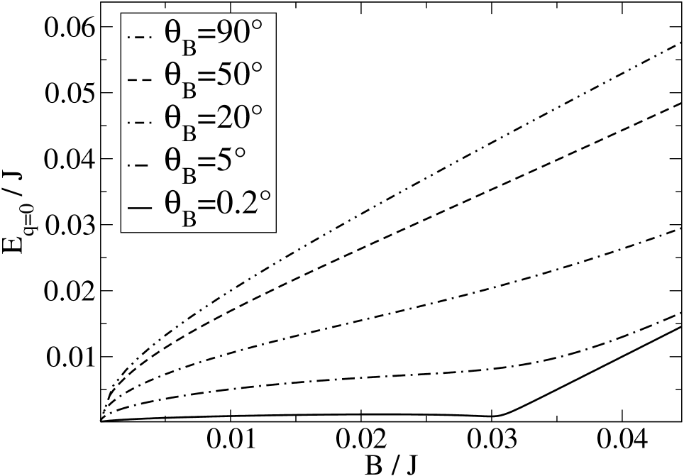
Figure 1: The energies of the uniform magnon mode $E_{\mathbf{q}=\mathbf{0}}(B)$ for different polar angles $\theta_{B}$ of the external field. $E_{\mathbf{q}=\mathbf{0}}$ is zero below $B/J\approx 0.03$ for $\theta_{B}=0^{\circ}$. The prefactors $g_{J}\mu_{B}$ and $k_{B}$ are absorbed in $B$ and $T$ respectively. The latter are given in units of the nearest neighbor Heisenberg coupling $J$. Parameters: $S=1$, $K/J=-0.03$ and $T/J=10^{-4}$.

This can be seen in Fig.1 where the uniform magnon modes $E_{\mathbf{q}=\mathbf{0}}(B)$ are shown for different orientations $\theta_{B}$, where $\theta_{B}$ is the polar angle of the external field. The integral (14) is now finite and a stable finite magnetization in the collinear phase having a well defined orientation in the $xz$-plane is possible.
Let us now come back to the case where the applied field is aligned in $z$-direction. It can be seen from Eq. (13) that for external field $B$ ($B\>||\>z$) larger than a critical field $B>B_{crit}$ given by:

$$B_{crit}\stackrel{{\scriptstyle!}}{{=}}|K_{eff}(T,B)|$$ (15)

a stable collinear solution exists.

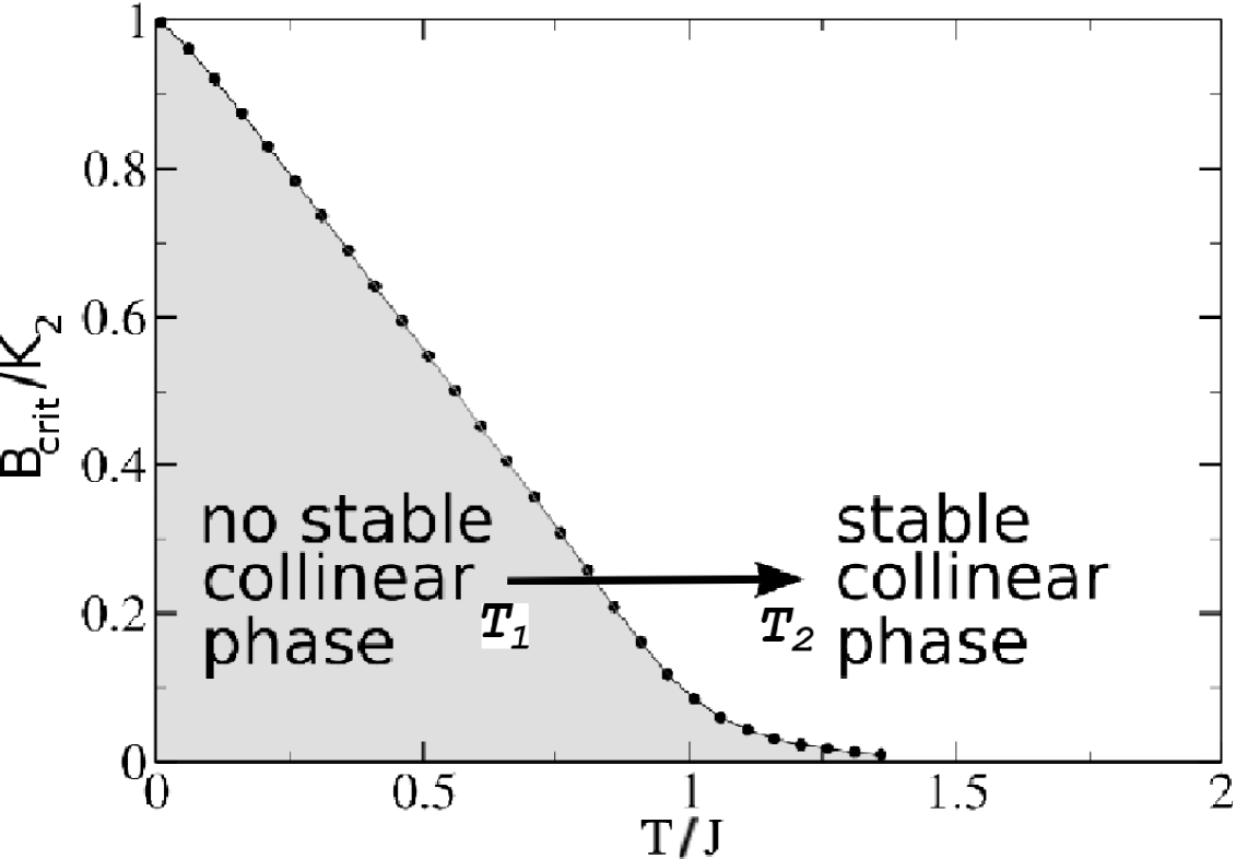
Figure 2: The normalized critical field $B_{crit}/K_{2}$ as a function of temperature. Parameters: $S=1$.

Since $K_{eff}(T)$ is a decreasing function of temperature $T$ a transition from non-collinear to collinear phase with increasing temperature is possible. In Fig. 2 we show the normalized critical field (15) $B_{crit}/K_{2}$ as a function of temperature $T$. For a constant magnetic field $B$ ($B\>||\>z$) at a temperature $T_{1}$ with $B<K_{eff}(T_{1},B)$ no stable collinear phase exist. Then by increasing the temperature up to $T_{2}$ the effective anisotropy $K_{eff}$ is sufficiently reduced such that $B>K_{eff}(T_{2},B)$, and the collinear phase becomes stable. Before we come to the results let us briefly sketch the main aspects of the QMC.

II.2 QMC

In the last section we gave a short description of the theory used to treat a system described by a Hamiltonian of form (1). This theory applies to the thermodynamic limit (films of infinte size) but contains certain approximations. Additionally the GFT is restricted to ordered phases with a collinear alignment of all spins. Therefore it would be very useful to have exact results at hand to crosscheck the predictions of GFT. A Quantum Monte Carlo method, particularly well suited for spin systems, is the stochastic series expansion (SSE) with directed loop update. We will sketch this method here only briefly as detailed descriptions can be already found elsewhere sandvik99 ; sandvik02 ; alet05 .

Our starting point is the series expansion of the partition function

$$\mathrm{Z}=\mathrm{Tr}e^{-\beta H}=\sum_{n=0}^{\infty}\sum_{\alpha}\frac{\beta^{n}}{n!}\langle\alpha|(-H)^{n}|\alpha\rangle$$ (16)

where $H$ denotes the Hamiltonian, $\{|\alpha\rangle\}$ are basis vectors of a proper Hilbert space and $\beta$ is the inverse temperature. The Hamiltonian is then rewritten in terms of bond Hamiltonians:

$$H=-J\sum_{b=1}^{M}H_{b}$$ (17)

where $H_{b}$ can be further decomposed into a diagonal and an off-diagonal part:

$$H_{D,b} = C+S_{i(b)}^{z}S_{j(b)}^{z}+b_{b}[S_{i(b)}^{z}+S_{j(b)}^{z}]$$

$$+k_{2b}[(S_{i(b)}^{z})^{2}+(S_{j(b)}^{z})^{2}]$$

$$H_{O,b} = \frac{1}{2}[S_{i(b)}^{+}S_{j(b)}^{-}+S_{i(b)}^{-}S_{j(b)}^{+}]$$ (19)

Here we have renormalized the anisotropy constant $k_{2b}$ and the magnetic field $b_{b}$ in such a way that (17) coincides with (1). $i(b)$ and $j(b)$ denotes the lattice sites connected by the bond $b$ and the additional constant $C$ in $H_{D,b}$ will be chosen such that all matrix elements of this term become positive, a condition necessary to interpret them as probabilities. Note that for a finite system at finite temperature the power series of the partition function can be truncated at a finite cutoff length $\Lambda$ without introducing any systematic error in practical computationssandvik02 . Therefore reinserting (17) into (16) and rewriting the result yields:

$$Z=\sum_{n=0}^{\Lambda}\sum_{S_{C_{\Lambda}}}\sum_{\alpha}\frac{\beta^{n}(\Lambda-n)!}{\Lambda!}\langle\alpha|S_{C_{\Lambda}}|\alpha\rangle.$$ (20)

Here $S_{C_{\Lambda}}$ denotes a product of operators (operator string) consisting of n non-unity operators and ($\Lambda-n$) unity operators $H_{0}=\mathrm{Id}$ which were inserted to get operator strings of equal length $\Lambda$.
In fact it is impossible to evaluate all operator strings in (20). The SSE-QMC replaces such an evaluation therefore by importance sampling over the strings according to their relative weight. Hence an efficient scheme for generating new operator strings is needed. In the directed loop version of the SSE this is done by dividing the update into two parts. In a first step a diagonal update is performed by traversing the operator string and replacing some unity operators by diagonal bond operators and vice versa (the probabilities for both substitutions have to fulfill the detailed balance criterion). Then the loop update follows in which new non-diagonal bond operators can appear in the operator string. For details of the update procedure we refer the interested reader to the according literature sandvik99 ; sandvik02 ; alet05 .
A full implementation of the SSE with directed loop update which we have used for all QMC calculations in this work can be found in the ALPS project ALPS ; alet05 . Since the SSE-QMC used by us is implemented in z-representation (spin quantization axis along z-axis) in-plane correlation functions e.g. the in-plane magnetization are not accessible. Further $B\>||\>z$ is the only possible field direction in the used QMC implementation because a traverse field (in-plane field component) would lead to non-closing loops (see Ref. qm, ).

III Results

As mentioned in Sec. II.1 the results for the in-plane systems are very sensitive to the effective anisotropy $K_{eff}(T)$. This sensitivity of the anisotropy is less pronounced for out-of-plane systems ($K_{2}>0$) since the applied field $B$ ($B\>||\>z$) and the intrinsic easy axis are parallel. In order to test our decoupling scheme (RPA+AC) we first compare GFT and QMC for an out-of-plane system.

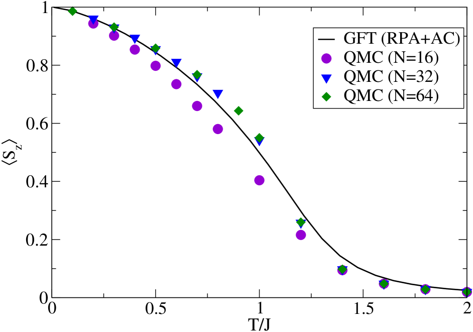
Figure 3: Magnetization vs. temperature for an out-of-plane easy-axis system ($K_{2}>0$). Straight line: GFT (RPA+AC) result; symbols: QMC results for different system sizes $N^{2}$. Parameters: $S=1$, $B/J=0.01$ ($B\>||\>z$) and $K_{2}/J=0.01$.

In Fig. 3 the magnetization $\langle S_{z}\rangle$ as a function of temperature $T$ is shown. The straight line belongs to the GFT whereas the symbols show the result of the QMC for different system sizes. Let us first comment on finite size effects in the QMC results.

It can be seen in Fig. 3 that the QMC results converge for increasing system size $N^{2}$ (for $N\times N$ square lattice). Indeed for $N\geq 32$ the QMC results are unbiased by finite size effects and resulting magnetization curves are almost equal for increasing $N\geq 32$. Note that we have omitted error bars in the figures showing QMC results because the relative errors are of the order $10^{-4}$.

We now compare the GFT with the QMC results ($N=64$). For low temperatures ($T/J\leq 0.5$) we obtain excellent quantitative agreement. This is plausible because in this region the GFT result coincides with the result of the spin-wave theory which is known to be reliable (exact for $T=0$) for low temperatures. For the intermediate region $T/J=0.5..1$ the RPA slightly underestimates the magnetization which was also found in Ref. qm, . The opposite is the case in the region near the extrapolated Curie temperature $T_{C}$ , where the magnetization is overestimated. The reason is the presence of longitudinal fluctuations, which play an important role in this region and it is well known that the RPA fails to treat them properly.

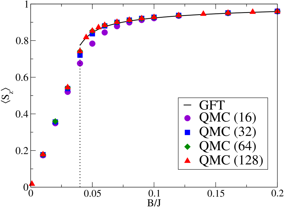
Figure 4: $z$-component of magnetization as a function of external magnetic field for fixed temperature $T/J=0.4$. In contrary to the GFT the magnetization obtained by QMC remains finite for all fields. The QMC results are converged for $N\geq 64$. Parameters: $S=1$, $K_{2}/J=-0.06$ and $\theta_{B}=0^{\circ}$.

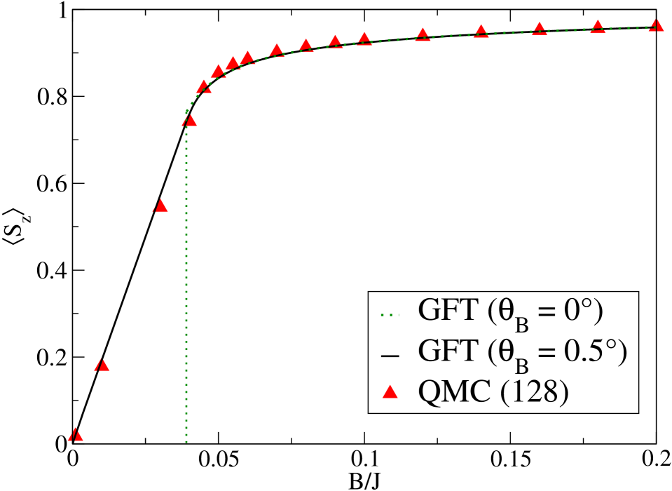
Figure 5: $z$-component of magnetization vs. external field for $T/J=0.4$ with slightly tilted field ($\theta_{B}=0.5^{\circ}$)in the GFT result (solid line). The dotted line shows GFT result for ($\theta_{B}=0^{\circ}$). Other parameters as in Fig. 4.

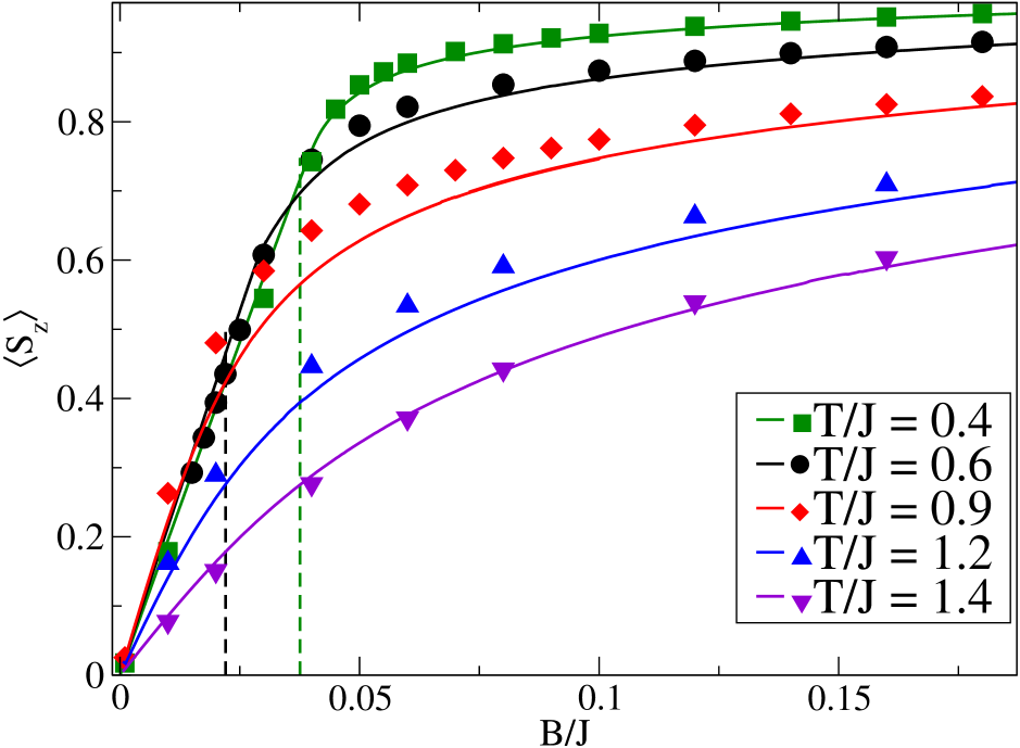
Figure 6: $z$-component of magnetization vs. external field for different temperatures $T/J$ and fixed system size $N^{2}$ ($N=128$). Solid lines: GFT ($\theta_{B}=0.5^{\circ}$), dashed lines: GFT ($\theta_{B}=0^{\circ}$) other parameters as in Fig. 4.

We consider now the case of in-plane systems ($K_{2}<0$) and applied field in the hard direction ($B\>||\>z$). As already mentioned there is no ’collinear’ magnetization in the GFT for $B_{z}<|K_{eff}(T)|$. In Fig. 4 the $z$-component of the magnetization is shown as a function of the external field $B$ for a constant temperature $T/J=0.4$. As in Fig. 3 we see that the QMC results for $N\geq 64$ are almost converged and the finite size of the calculated system in QMC should not influence the results anymore. The dotted line marks a critical field $B_{crit}$. For magnetic fields larger than the critical one $B>B_{crit}$ we obtain good agreement between QMC and GFT results. Below the critical field $B<B_{crit}$ GFT does not yield a stable homogeneous magnetization. However the QMC results show that there is a finite $z$-component of the magnetization in the considered system for $0\leq B\leq B_{crit}$.
In order to compare QMC with GFT results we have tilted the magnetic field by $\theta_{B}=0.5^{\circ}$ which corresponds to $B_{x}<10^{-2}B_{z}$ in the GFT. As explained before any symmetry breaking field $B_{x}\neq 0$ leads to a stable homogeneous magnetization with well-defined orientation in the $xz$-plane. However such a small contribution of the external field within the plane should hardly influence the $z$-component of the magnetization. This is confirmed by Fig. 5 where we show QMC results ($N=128$, $\theta_{B}=0^{\circ}$) as well as the corresponding GFT results with $\theta_{B}=0^{\circ}$ and $\theta_{B}=0.5^{\circ}$. As expected for $|B|>B_{crit}$ the two solutions in the GFT are nearly the same and agree well with QMC. Below the critical field only the solution with the slightly tilted field yields a stable homogeneous magnetization and its $z$-component compares well with the QMC result in the untilted case.
The above results can be interpreted within a semi-classical picture of non-collinear vortex configurations which are stable below a critical field $B_{crit}$ in $z$-direction and contribute a finite $z$-component to the magnetization in case of an applied field. ivanov02 Despite the lack of direct, quantitative access to such states (or corresponding physical in-plane observables) within the QMC algorithm they are included in principle and one can observe their consequences, namely a finite $z$-component of the magnetization below the critical GFT field. On the other hand GFT can only describe homogeneous collinear configurations of spins therefore showing a breakdown of magnetization. However by applying a small field in $x$-direction the $xy$-symmetry is broken and the spins rotate in the field direction (the vortices vanish) and the collinear phase is retrieved. Our results corroborate this interpretation based on the classical picture. Let us emphasize that both, GFT for slightly tilted field and QMC for $B\;||\;z$, describe the competition between the external field (which favors magnetization parallel to $z$) and the anisotropy favoring in-plane magnetization. Comparing the $z$-components of the magnetization for both cases, one can conclude that the ratio of the competing forces are comparable for QMC and GFT. This indicates that this competition is correctly taken into account in GFT.
In Fig. 6 the same field dependence of the $z$-component of the magnetization is shown for different temperatures. We have plotted the result for the tilted field in case of GFT, the point of breakdown in the untilted case is indicated by the dotted line. It can be seen that for higher temperatures no breakdown of collinear magnetization occurs, meaning that the condition for the critical field ($B\leq|K_{eff}(T,B)|$) is never fulfilled in this case. The discrepancies at intermediate temperatures ($T=0.9..1.2$) are due to the RPA decoupling in the GFT as was discussed already.

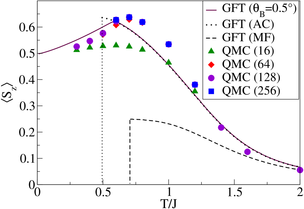
Figure 7: The $z$-component of magnetization as function of temperature for a fixed external field. Below a critical temperature $T_{crit}$ there is a breakdown of magnetization in GFT where is no in QMC. Parameters: $B/J=0.03$, $S=1$, $K_{2}/J=-0.06$.

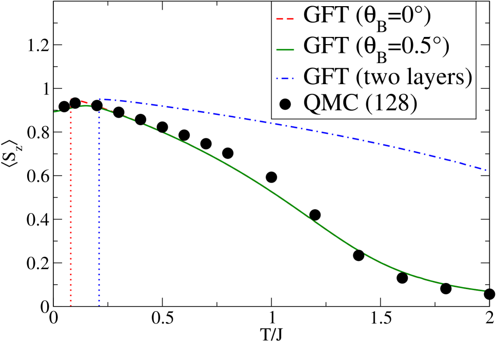
Figure 8: Same situation as in Fig. 7 for $K_{2}/J=-0.04$ (other parameters as in Fig.7). The result for a two layer film treated by GFT is plotted also (dashed-dotted line).

In Figs. 7, 8 and 9 the $z$-component of the magnetization is plotted as a function of temperature obtained by GFT (straight line RPA+AC) as well as QMC (symbols) for different system sizes and a constant applied magnetic field.
Let us first discuss the qualitative behavior of the magnetization as a function of temperature which is found in all three figures. For high $T$ ($T\gg T_{crit}$) the magnetization is reduced by thermal fluctuations (where the tail of the curve above $T/J\approx 1.5$ is due to the applied external field). In the vicinity of $T_{crit}$, $T-T_{crit}\rightarrow 0^{+}$, a competition between two effects sets in and has a pronounced influence on the magnetization. On the one side the effective anisotropy acts against the external field ($B_{eff}=B-|K_{eff}(T)|$, ($B\>||\>z$)). The effective anisotropy $K_{eff}(T)$ is reduced with increasing temperature $T$ and thus the effective field $B_{eff}$ increases with $T$. This effect tends to enhance the magnetization with $T$. On the other side thermal fluctuations suppress the magnetization with increasing $T$. The flattening of the magnetization curve near $T_{crit}$ is a result of this competition. For low temperatures $T<T_{crit}$ the effective anisotropy in the GFT cannot be overcome by the external field ($B<|K_{eff}(T)|$, ($B\>||\>z$)). Therefore the collinear magnetization in our approximation vanishes due to the mentioned gapless excitations, in contrast to QMC which yields again a finite magnetization because non-collinear states are taken into account as discussed above. The reduction of the $z$-component of magnetization in QMC below $T_{crit}$ can be pictured classically as the spins being in a non-collinear phase with an angle $\theta$ with respect to the $z$-axis. Since in general anisotropy effects (which favor in-plane magnetization) increase when temperature is lowered the $z$-component of the magnetization decreases.

Now we discuss the three figures in detail. In Fig. 7 we have plotted QMC results for different system size showing again that these are well converged for $N\geq 64$. Thus we conclude that the striking difference between GFT and QMC is not a mere finite size effect. The breakdown of magnetization in GFT occurs at a critical temperature $T_{crit}/J=0.5$ whereas no such breakdown exists in QMC. However the exposed maximum of the magnetization in QMC lies near the breakdown point. The differences between QMC and GFT in the temperature range $T/J\approx 0.3\dots 1.3$ are due to the decoupling of the exchange and anisotropy term in GFT as also seen in Fig. 3. It is worth mentioning that the value of the z-component of the magnetization is nearly the same at the breakdown point in GFT and the maximum in the QMC. Thus we have the result that although GFT cannot describe the non-collinear phase by ansatz its breakdown coincides rather well with the onset of this phase, which we attribute to the maximum of the QMC curve. Fig.8 shows the same situation for a different anisotropy constant $K_{2}=-0.04$. The critical temperature is lower than in Fig.7 since the ratio $B_{z}/K_{2}$ becomes larger.

Figure 9: Same situation as in Fig. 7 for $K_{2}/J=-0.01$, $B/J=0.005$ and slightly tilted field ($\theta_{B}=0.5^{\circ}$) for the GFT results.

The tilted field case is also shown for the GFT results. Again the qualitative agreement of the $z$-component of magnetization with QMC is good. To confirm this point we have plotted the temperature dependence for an other set of parameters in Fig. 9. There is as good qualitative agreement of the two approaches. Additionally one gets a finite component in $x$-direction in GFT which is also plotted in the figure. The two effects of the external field vs. anisotropy competition are nicely to be seen: a non-collinear state for $B\;||\;z$ ($z$-component only in QMC but not in GFT) and rotation of magnetization for slightly tilted external field (seen only in GFT). The ratio of the competing forces agree well again in both treatments.

In Fig. 7 we have plotted the results of a different decoupling scheme of the anisotropy terms (namely a mean field decoupling, dashed line in Fig. 7). Although the overall characteristic resembles the RPA$+$AC result (breakdown of magnetization) the mean field results differ extremely from the QMC for a large range of temperature and underestimates the magnetization. This demonstrates the reliability of the Anderson-Callen treatment of the local anisotropy terms presented in Refs. schwieger1, ; schwieger2, ; dipolpaper, ; pini, .

The extension of the GFT method to multi-layer films is straightforward.schwieger2 We have also included results for a two-layer film in Fig. 8 for the same parameters as in the monolayer case. One finds that for a double layer magnetism is stabilized, which can be attributed to the increased coordination number and thus higher exchange energy. Just like for a monolayer, one observes a breakdown of collinear magnetization at some critical temperature. This is due to the fact that the same reasoning regarding the vanishing excitation gap also applies for multilayer (slab) systemsaxel00 . The effective anisotropy per layer is essentially the same as for a single layer, thus the critical $\langle S_{z}\rangle$-value (magnetization at critical field $B_{crit}$) is practically the same. The critical temperature is higher than that of a monolayer due to the increased magnetic stiffness of the double layer.

IV Summary and Conclusions

Using GFT and QMC calculations we studied easy-plane systems as well as easy-axis systems with an external field applied perpendicularly to the film. The GFT treatment of the Hamiltonian Eq. (1) consists of a RPA-decoupling for the nonlocal terms and an AC-decoupling for the local terms performed in a rotated frame, where the new $z^{\prime}$-axis is parallel to the magnetization. For the QMC calculations we have used the stochastic series expansion (SSE) with directed loop updates, which is well suited for spin-systems.
We have calculated the magnetization as a function of the external field as well as temperature. We found a critical field and critical temperature respectively below which is no magnetization in GFT whereas there is one in QMC. By tilting the field slightly in GFT so that it has a small component in $x$-direction we get a stable magnetization even below the critical field or temperature. The $z$-component of the magnetization in this case coincides well with the $z$-component obtained by QMC for the untilted field confirming that GFT and QMC agree well in the description of the external field vs. anisotropy competition. However, this comparison can be only somewhat indirect, since QMC has access to the non-collinear ($B\;||\;z$) state only, while GFT is limited to collinear ferromagnetic states (rotated homogeneous magnetization) found for slightly tilted external fields.
For parameters that are accessible by both QMC and GFT ($B\;||\;z$; $B>B_{crit}(T)$) QMC and GFT are in good agreement. Thus one can conclude that the GFT is applicable to the homogeneous phases of systems described by Eq. (1) and can be used also for system configurations not accessible by QMC due to too large system size as e.g. multilayer systems.
It would be an interesting task for a succeeding work to extend the GFT in order to get a deeper insight into the non-collinear configurations also.

Appendix A magnetization angle

Here we will discuss the second mathematical solution which occurs besides Eq. 10. For an external field in the $z$-direction the angle dependent part of the free energy including second order anisotropy can be expanded as lindner ; farle :

$$F=-M_{z}B_{z}\cos\theta-\tilde{K}_{2}\cos^{2}\theta$$

where $M_{z}$ is the $z$-component of the magnetization and $\tilde{K}_{2}$ is the first nonvanishing coefficient in an expansion of the free energy for a system with second order anisotropy. For the equilibrium angle one gets:

$$\frac{\partial F(\theta)}{\partial\theta} = M_{z}B_{z}\sin\theta+2\tilde{K}_{2}\cos\theta\sin\theta\stackrel{{\scriptstyle!}}{{=}}0.$$ (21)

Therefore one gets two solutions for in-plane systems ($\tilde{K}_{2}<0$). For $\sin\theta\neq 0$ one gets immediately the solution of Eq. 10 if $2\tilde{K}_{2}/M_{z}\equiv K_{eff}$ holds. This is the stable solution. The trivial (second) solution $\sin\theta=0$ is unstable for $B_{z}<|K_{eff}|$ because

$$\frac{\partial^{2}F(\theta)}{\partial\theta^{2}}\mid_{\sin\theta=0} = \left\{\begin{array}[]{cc}<0&~{}~{}\text{for}~{}~{}B_{z}<|K_{eff}|\\ >0&\text{otherwise}\end{array}\right.$$ (24)

holds. For a detailed discussion of stability conditions in film systems we refer to Refs. farle, ; lindner, .

References

- (1) M. Farle, B. Mirwald-Schulz, A. N. Anisimov, W. Platow, and K. Baberschke, Phys. Rev. B 55, 3708 (1997).
- (2) A. Hucht and K. D. Usadel, Phys. Rev. B 55, 12309 (1997).
- (3) P. J. Jensen and K. H. Bennemann, Solid State Comm. 105, 577 (1998), and references therein.
- (4) R. P. Erickson and D. L. Mills, Phys. Rev. B 44, 11825 (1991).
- (5) D. K. Morr, P. J. Jensen, and K. H. Bennemann, Surf. Sci. 307-309, 1109 (1994).
-
(6)
P. Politi, A. Rettori, M. G. Pini, and D. Pescia,
J. Magn. Magn. Mater. 140-144, 647 (1995);
A. Abanov, V. Kalatsky, V. L. Pokrovsky and W. M. Saslow, Phys. Rev. B 51, 1023 (1995). -
(7)
A. Hucht, A. Moschel, and K. D. Usadel,
J. Magn. Magn. Mater. 148, 32 (1995);
S. T. Chui, Phys. Rev. B 50, 12559 (1994). - (8) T. Herrmann, M. Potthoff, and W. Nolting, Phys. Rev. B 58, 831 (1998).
- (9) P. Henelius, P. Fröbrich, P. J. Kuntz, C. Timm, and P. J. Jensen, Phys. Rev. B 66, 094407 (2002).
- (10) S. Schwieger, J. Kienert, and W. Nolting, Phys. Rev. B 71, 024428 (2005).
- (11) S. Schwieger, J. Kienert, and W. Nolting, Phys. Rev. B 71, 174441 (2005).
- (12) F. Körmann, S. Schwieger, J. Kienert, and W. Nolting, Eur. Phys. J. B 53, 463 (2006).
- (13) M. G. Pini, P. Politi and R. L. Stamps, Phys. Rev. B 72, 014454 (2005).
- (14) J. M. Kosterlitz and D. J. Thouless, J. Phys. C 6, 1181 (1973).
- (15) G. M. Wysin, Phys. Lett. A 240, 95 (1998).
- (16) E. Yu. Vedmedenko, A. Ghazali, and J. -C. S. Lévy, Phys. Rev. B 59, 3329 (1999).
- (17) K. W. Lee and C. E. Lee, Phys. Rev. B 70, 144420 (2004).
- (18) M. Rapini, R. A. Dias, and B. V. Costa, Phys. Rev. B 75, 014425 (2007).
- (19) B. A. Ivanov and G. M. Wysin, Phys. Rev. B 65, 134434 (2002).
- (20) F. Bloch, Z. Phys. 61, 206 (1930).
- (21) P. Bruno, Phys. Rev. B 43, 6015 (1998).
- (22) P. J. Jensen and K. H. Bennemann, in Magnetism and electronic correlations in local-moment systems, edited by M. Donath, P. A. Dowben and W. Nolting, p.113 (World Scientific, 1998).
- (23) P. Fröbrich, P. J. Jensen, and P. J. Kuntz, Eur. Phys. J. B 13, 477 (2000).
- (24) N. N. Bogolyubov and S. V. Tyablikov, Soviet. Phys.-Doklady 4, 589 (1959).
- (25) F. B. Anderson and H. Callen, Phys. Rev. 136, A1068 (1964).
- (26) P. Fröbrich and P. J. Kuntz, http://arxiv.org/pdf/cond-mat/0607675.
- (27) J. Lindner, Ph.D. thesis, Freie Universität Berlin (2002).
- (28) A. W. Sandvik, Phys. Rev. B 59, R14 157 (1999).
- (29) O. F. Syljuåsen and A. W. Sandvik, Phys. Rev. E 66, 046701 (2002).
- (30) F. Alet, S. Wessel, and M. Troyer, Phys. Rev. E 71, 036706 (2005).
- (31) ALPS collaboration, J. Phys. Soc. Jpn. Suppl. 74, 30 (2005). Source codes can be obtained from http://alps.comp-phys.org/
- (32) A.Gelfert and W.Nolting, Phys. Stat. Sol. B 217, 805 (2000).