Compton Scattering of Fe K$\alpha$ Lines in Magnetic Cataclysmic Variables

Abstract

Compton scattering of X-rays in the bulk flow of the accretion column in magnetic cataclysmic variables (mCVs) can significantly shift photon energies. We present Monte Carlo simulations based on a nonlinear algorithm demonstrating the effects of Compton scattering on the H-like, He-like and neutral Fe K$\alpha$ lines produced in the post-shock region of the accretion column. The peak line emissivities of the photons in the post-shock flow are taken into consideration and frequency shifts due to Doppler effects are also included. We find that line profiles are most distorted by Compton scattering effects in strongly magnetized mCVs with a low white dwarf mass and high mass accretion rate and which are viewed at an oblique angle with respect to the accretion column. The resulting line profiles are most sensitive to the inclination angle. We have also explored the effects of modifying the accretion column width and using a realistic emissivity profile. We find that these do not have a significant overall effect on the resulting line profiles. A comparison of our simulated line spectra with high resolution Chandra/HETGS observations of the mCV GK Per indicates that a wing feature redward of the 6.4 keV line may result from Compton recoil near the base of the accretion column.

1 Introduction

Magnetic cataclysmic variables (mCVs) are close interacting binaries consisting of a magnetic white dwarf (WD) and a low mass red dwarf (Warner, 1995). Near the white dwarf surface the accretion flow in mCVs is confined by the magnetic field of the WD and is channelled to the magnetic pole region(s) of the WD, forming an accretion column (see Warner, 1995; Cropper, 1990; Wu, 2000; Wu et al., 2003, for reviews).

Near the base of the accretion column, material in supersonic free-fall is brought to rest on the WD surface, forming a standing shock which heats and ionizes the accreting plasma. The shock temperature $T_{\rm s}$ depends mainly on the mass $M_{\rm wd}$ and radius $R_{\rm wd}$ of the WD and is given by (e.g. Wu, 2000)

$$kT_{\rm s}=\frac{3}{8}\frac{GM_{\rm wd}{\mu}m_{\rm H}}{R_{\rm wd}+x_{\rm s}}\qquad,$$ (1)

where $\mu$ is the mean molecular weight and $x_{\rm s}$ is the shock height. For WD masses $\mbox{$M_{\rm wd}$}\approx(0.5-1.0)\,\mbox{$M_{\sun}$}$ and typical mCV parameters, the shock temperature is $kT_{\rm s}\approx(10-40)\,\rm keV\approx(1-4)\times 10^{8}$ K. The plasma in the post-shock region of the column cools by emitting bremsstrahlung X-rays and optical/IR cyclotron radiation (Lamb & Masters, 1979; King & Lasota, 1979). Since cooling occurs along the flow, the post-shock region is stratified in density and temperature. The height of the post-shock region is determined by the cooling length. For a flow with only bremsstrahlung cooling, the shock height is given by (Wu, Chanmugam & Shaviv, 1994)

$$x_{\rm s}\approx 3\times 10^{7}\left(\frac{\dot{m}}{1\,\rm\mbox{$\rm g\,cm^{-2}\,s^{-1}$}}\right)\left(\frac{\mbox{$M_{\rm wd}$}}{0.5\,\mbox{$M_{\sun}$}}\right)^{3/2}$$

$$\times\left(\frac{\mbox{$R_{\rm wd}$}}{10^{9}\rm cm}\right)^{-3/2}{\rm cm}$$ (2)

where $\dot{m}$ is the specific mass accretion rate.

A plasma temperature of $kT\approx 10$ keV is sufficient to fully ionize elements such as argon, silicon, sulphur, aluminium or calcium. Heavier elements such as iron can be highly ionized, resulting in H-like Fe XXVI and He-like Fe XXV ions. K-shell transitions in Fe XXVI and Fe XXV ions give rise to K$\alpha$ lines at 6.97 keV and 6.675 keV, respectively (see e.g. Wu, Cropper & Ramsay, 2001). The irradiation of low ionized and neutral iron by X-rays above the Fe K edge produces fluorescent K$\alpha$ emission at approximately 6.4 keV inside the WD atmosphere, beneath the accretion column and in surrounding areas. The natural widths of the Fe K$\alpha$ lines are small, but the lines can be Doppler broadened by the bulk and thermal motions of the emitters in the post-shock flow. The bulk velocity immediately downstream of the shock is $\approx 0.25\left(G\mbox{$M_{\rm wd}$}/\mbox{$R_{\rm wd}$}\right)^{1/2}\sim 1000\,\rm km\,s^{-1}$ for typical mCV parameters. Lines can also be broadened by scattering processes. Compton (electron) scattering is expected to be more important than resonance (ion) scattering for the K$\alpha$ transitions (Pozdnyakov, Sobol & Sunyaev, 1983). For an mCV with specific accretion rate $\dot{m}\sim 10~{}\mbox{$\rm g\,cm^{-2}\,s^{-1}$}$ the electron number density is $n_{\rm e}\sim 10^{16}\rm\,cm^{-3}$ for a shock heated region of thickness $x_{\rm s}\sim 10^{7}\rm\,cm$, giving a Thompson optical depth of $\tau\sim 0.1$. Thus, one in every ten photons would encounter an electron before leaving the post-shock region. The relative importance of Doppler shifts, thermal Doppler broadening and Compton scattering depends on the ionization structure in the post-shock flow.

X-ray observations by Chandra/HETGS and ASCA/SIS have revealed significant broadening of some Fe K$\alpha$ lines in mCVs (Hellier, Mukai, & Osborne,, 1998; Hellier & Mukai, 2004). It was suggested that Compton scattering in the accretion column is largely responsible for the broadening in the observed lines. Doppler broadening should only be significant in lines emitted close to the shock. The absence of Doppler shifts in the observed H-like and He-like lines suggests that these photons may be emitted predominantly from regions of lower velocity near the base of the accretion column (Hellier & Mukai, 2004). The observed line profiles have yet to be fully interpreted with a quantitative model that takes into account Compton scattering effects in a complex ionization structure.

In this paper, we study the effects of Compton scattering in the accretion column of mCVs using a nonlinear Monte Carlo algorithm (Cullen, 2001a, b) that self-consistently takes into account the density, velocity and temperature structure in the column (Wu et al., 2001). The effects of dynamical Compton scattering are also included. In a preliminary investigation (Kuncic, Wu & Cullen, 2005), it was found that Fe K$\alpha$ line photons emitted from the dense base of the accretion column undergo multiple Compton scatterings and as a result, the base of the line profile is substantially broadened. Photons emitted near the shock can also undergo scatterings with hot electrons immediately downstream of the shock, as well as cold electrons in the pre-shock flow before escaping the column. The resulting line profiles display a shoulder-like feature redward of the line centre. More significant broadening is observed when cyclotron cooling is sufficiently strong to produce a dense, compact post-shock region (see Wu, 2000, for example). Here, we make three substantial improvements to the previous study: (i) we include Doppler effects; (ii) the photon source regions in the post-shock column are determined from the ionization structure, rather than specified arbitrarily; and (iii) the effects of different viewing angles are fully explored. The paper is organized as follows: the theoretical outline and geometry of the model are described in Section 2. Numerical results for cases where cyclotron cooling is negligible and when it dominates are presented and discussed in Section 3. A summary and conclusions are presented in Section 4.

2 Theoretical Model

2.1 Physical Processes

Line photons can undergo energy changes when scattering with electrons, resulting in distortions in the line profile. The energy change of a photon per scattering is given by (e.g. see Pozdnyakov et al., 1983),

$$\frac{E^{\prime}}{E}=\frac{1-{\mu}{\beta}}{1-{\mu}^{\prime}{\beta}+\frac{E}{{\gamma}m_{\rm e}c^{2}}(1-{\cos}{\alpha})}$$ (3)

where E is the initial photon energy, $\gamma m_{\rm e}c^{2}$ is the electron energy, with $\gamma=(1-\beta^{2})^{-1/2}$ and where $\beta=v/c$ includes both thermal and bulk motion, $\theta=\cos^{-1}{\mu}$ is the incident photon propagation angle measured relative to the electron’s direction of motion, and the scattering angle is $\alpha$. The prime superscript denotes quantities after a scattering event. Although the energy change per scattering is typically small, the line profile can be broadened considerably as a result of multiple scatterings if the optical depth is large.

Photons scattering with hot electrons (i.e. $kT_{\rm e}>E_{\rm c}$ where $T_{\rm e}$ is the electron temperature and $E_{\rm c}$ is the line centre energy) will gain energy, while photons scattering with cold electrons ($kT_{\rm e}\ll E_{\rm c}$) will lose energy due to recoils. In the mCV context, Compton recoil can be important for photons scattering with electrons in the cold pre-shock flow and also near the base of the column, where $\beta$ rapidly decreases and where the optical depth is high. From equation (3), the fractional energy change due to Compton recoil $\left(E\gg\gamma m_{\rm e}c^{2}\right)$ is

$$\frac{{\Delta}E}{E}\simeq-\frac{E}{m_{\rm e}c^{2}}(1-\cos\alpha)\qquad.$$ (4)

In the post-shock accretion column in mCVs, line photons undergo thermal Doppler broadening as well as Doppler shifts. The bulk velocity of the accreting material immediately downstream of the shock is $\sim 1000\,\rm km\,s^{-1}$. For all inclination angles $i$ (see Figure 1), the bulk flow is moving away from our line of sight, so the line centre energy is redshifted by an amount $\Delta E/E\sim\beta\cos i$. However, since the bulk velocity in the post-shock flow in mCVs is always less than a few $\times\,1000\,\rm km\,s^{-1}$, giving $\beta<10^{-2}$, Doppler shifts are expected to be negligible. Thermal Doppler broadening, on the other hand, is expected to be of order ${\Delta}E/E\sim\sqrt{(2kT_{\rm s}/m_{\rm i}c^{2})}\approx 0.002$ for lines emitted in the hottest regions of the post-shock flow (i.e. immediately downstream of the shock), where $m_{\rm i}$ is the mass of the ion.

In strongly magnetized mCVs, cyclotron emission is the dominant cooling process. The effect of this additional electron cooling process in the post-shock region is to reduce the shock height and modify the density and temperature structure of the region (Wu et al., 1994). This can enhance Compton scattering features in line profiles (Kuncic et al., 2005).

2.2 Geometry of the Accretion Column

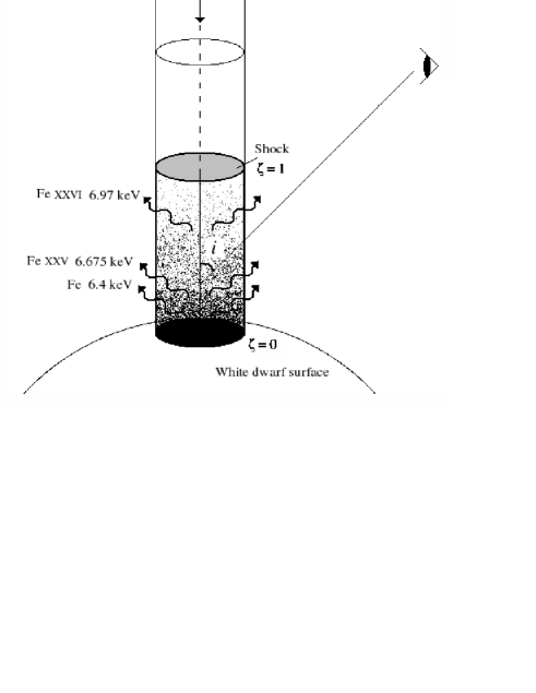
Figure 1: Schematic illustration of the geometry of the magnetized white dwarf accretion column showing approximate locations of Fe K$\alpha$ source regions.

The geometry of an mCV accretion column is shown in figure 1. The column is modelled as a cylinder and is divided into a shock heated region and a cool pre-shock region. In the pre-shock region, the density and velocity of the accreting material are constant. The velocity of the pre-shock flow is approximated by the free-fall velocity at the shock height, $\mbox{$v_{\rm ff}$}(x_{\rm s})=[G\mbox{$M_{\rm wd}$}/(\mbox{$R_{\rm wd}$}+x_{\rm s})]^{1/2}$, and the plasma is assumed to be cold ($kT_{\rm e}\ll 1\rm~{}keV$). The electron number density in the pre-shock flow is $n_{\rm e}=\dot{m}/({\mu}m_{\rm H}\mbox{$v_{\rm ff}$})$, where $\dot{m}$ is the specific mass accretion rate. In the post-shock region, the density, velocity and temperature profiles are calculated using the hydrodynamic solution described in Wu et al. (1994), for bremsstrahlung and cyclotron cooling. The parameters that determine the structure of the post-shock region are the WD mass $M_{\rm wd}$, the WD radius $R_{\rm wd}$, the specific mass accretion rate $\dot{m}$ and the ratio of the efficiencies of cyclotron cooling to bremsstrahlung cooling $\epsilon_{\rm s}$.

The accretion column is viewed from an inclination angle $i$, measured relative to the column axis (see Fig. 1). An inclination angle $i=0^{\scriptscriptstyle{\circ}}$ corresponds to viewing the column along its axis, towards the WD, while viewing the column from an inclination angle $i=90^{\scriptscriptstyle{\circ}}$ is equivalent to viewing the column from the side.

The line photons are injected into the post-shock region at a specific dimensionless height $\zeta\equiv{x}/{x_{\rm s}}$ at or above the WD surface, where ${\zeta}=0$ and ${\zeta}=1$ correspond to the WD surface and shock surface, respectively (see Fig. 1). For each set of mCV parameters, the injection point of the line corresponds to the location in the post-shock region where the emissivity of the specific line peaks, according to the ionization structure determined by Wu et al. (2001). The bulk and thermal velocities at the line injection height $\zeta$ are used to calculate the Doppler shift and broadening of the lines.

The Monte Carlo technique is used to model Compton scattering effects on photon propagation in the column. The distance to a tentative scattering point is determined using an algorithm based on a nonlinear transport technique (Stern et al., 1995) which integrates the mean free path over the spatially varying electron density (Cullen, 2001a, b). The scattering cross-section is determined from the Klein-Nishina formula and the momentum vector at the scattering point is drawn from an isotropic Maxwellian distribution at the local temperature. A rejection algorithm is used to decide whether the scattering is accepted (Cullen, 2001b). For an accepted event the energy and momentum changes of the photon are calculated as described in Pozdnyakov et al. (1983). In each simulation photons are followed until they leave the column and binned to form a spectrum. A full description of the numerical algorithm can be found in Cullen (2001a).

In the simulations described below, we make the following simplifying assumptions: a fixed number of $10^{8}$ photons are used to simulate each line; a single energy is used for each line (whereas in reality, the neutral and Lymann $\alpha$ transitions are doublets, with energies 6.391/6.404 keV and 6.952/6.973 keV, and the He-like transition has both resonant, inter-combination and forbidden components); a fixed accretion column width is used and a single line injection site is used.

3 Results and Discussion

Figure 2: The profiles of (a) electron temperature $T_{\rm e}$, (b) mass density $\rho_{\rm e}$ and (c) bulk velocity $v_{\rm b}=\beta_{\rm b}c$ in the post-shock accretion column of an mCV with $\mbox{$M_{\rm wd}$}=0.5\,\mbox{$M_{\sun}$}$ and $\dot{m}=10\rm\,\mbox{$\rm g\,cm^{-2}\,s^{-1}$}$. $\zeta=0$ corresponds to the base of the accretion column and $\zeta=1$ to the shock. The solid line shows the profile for the case where the ratio of cyclotron to bremsstrahlung cooling at the shock is $\epsilon_{\rm s}=0$, the dotted line for $\epsilon_{\rm s}=10$ and the dashed line for $\epsilon_{\rm s}=100$. In (a) the corresponding mean thermal electron velocity $\beta_{\rm e}=v_{\rm e}/c$ is also shown as a function of $\zeta$.

We present simulations of Compton scattering of Fe K$\alpha$ lines in an mCV accretion column for two different WD mass-radius values: $\mbox{$M_{\rm wd}$}=0.5\,\mbox{$M_{\sun}$},\,\mbox{$R_{\rm wd}$}=9.2\times 10^{8}\rm\,cm$ and $\mbox{$M_{\rm wd}$}=1.0\,\mbox{$M_{\sun}$},\,\mbox{$R_{\rm wd}$}=5.5\times 10^{8}\rm\,cm$ (Nauenberg, 1972). For each mass, we consider two different specific mass accretion rates, $\dot{m}=1~{}\mbox{$\rm g\,cm^{-2}\,s^{-1}$}$ and $\dot{m}=10~{}\mbox{$\rm g\,cm^{-2}\,s^{-1}$}$, and inclination angles $i=0^{\scriptscriptstyle{\circ}}$, $45^{\scriptscriptstyle{\circ}}$ and $90^{\scriptscriptstyle{\circ}}$ with $\pm 5^{\scriptscriptstyle{\circ}}$ range. The cross-sectional radius of the accretion column is fixed at $0.1\mbox{$R_{\rm wd}$}$. We investigate the effect of varying the column width in section 3.3.

Figure 2 shows the temperature, velocity and density profiles of an accretion column for an mCV with WD mass $M_{\rm wd}=0.5\,\mbox{$M_{\sun}$}$ and $\dot{m}=10~{}\mbox{$\rm g\,cm^{-2}\,s^{-1}$}$, for cases where the ratio of cyclotron to bremsstrahlung cooling at the shock is $\epsilon_{\rm s}=$ 0, 10, and 100. The temperature decreases monotonically from a shock temperature $kT_{\rm s}\approx 14\,\rm keV$ ($\zeta=1$), to a small finite value at the base of the column ($\zeta=0$).The mass density in the post-shock region is determined by $\rho(\zeta)=4\dot{m}/v_{\rm b}(\zeta)$ and is a minimum at the shock and reaches a maximum at the base of the column. The bulk velocity of the accreting material at the shock is $0.25\mbox{$v_{\rm ff}$}$ and decreases to zero at the base of the column, where the plasma settles on the WD surface.

Figures 3 and 4 show the simulated line spectra for the case where cyclotron cooling is negligible and bremsstrahlung cooling dominates ($\epsilon_{\rm s}=0$). Figure 5 shows the simulated profiles for $\mbox{$M_{\rm wd}$}=0.5\,\mbox{$M_{\sun}$}$ and $\mbox{$M_{\rm wd}$}=1.0\,\mbox{$M_{\sun}$}$ when cyclotron cooling dominates bremsstrahlung ($\epsilon_{\rm s}=10$). In these cases, the neutral Fe K$\alpha$ line is emitted at the WD surface ($\zeta=0$), where the bulk velocity is approximately zero and the thermal velocity of the plasma is small. The 6.675 keV Fe K$\alpha$ line is emitted from the lowest few percent of the column ($\zeta\sim 0.003$) where the velocity of the infalling material and the thermal electron velocity are still relatively small. These lines thus show very little Doppler broadening. The 6.97 keV line, however, is emitted much closer to the shock ($\zeta\sim 0.16$), in regions where the temperature of the accreting material is considerably higher and thus suffers more substantial Doppler broadening (see Wu et al., 2001). The simulated line spectra for the case where the accretion column radius is fixed at $4.6\times 10^{7}\,\rm cm$ is shown in Figure 6. Figure 7 shows the simulated profiles for the case where the line photon injection along the flow is specified according to the emissivity profile model of Wu et al. (2001). In figure 8 we compare our simulated line spectra with an observation of the mCV GK Per detected by Chandra/HETGS.

Table 1 shows a comparison of the FWHM of the Fe K$\alpha$ lines for $\mbox{$M_{\rm wd}$}=1.0\,\mbox{$M_{\sun}$}$ and $\mbox{$M_{\rm wd}$}=0.5\,\mbox{$M_{\sun}$}$ with low and high $\dot{m}$ and for $\epsilon_{\rm s}=0$ and $\epsilon_{\rm s}=10$.

3.1 No Cyclotron Cooling

(a) $\mbox{$M_{\rm wd}$}=1.0\,\mbox{$M_{\sun}$}$, $\dot{m}=1~{}\mbox{$\rm g\,cm^{-2}\,s^{-1}$}$, $kT_{\rm s}=34\,\rm keV$, no cyclotron cooling (b) $\mbox{$M_{\rm wd}$}=1.0\,\mbox{$M_{\sun}$}$, $\dot{m}=10~{}\mbox{$\rm g\,cm^{-2}\,s^{-1}$}$, $kT_{\rm s}=46\,\rm keV$, no cyclotron cooling

Figure 3: Profiles of Fe K$\alpha$ lines scattered by electrons in the accretion column of an mCV with $\mbox{$M_{\rm wd}$}=1.0\,\mbox{$M_{\sun}$}$ and with (a) $\dot{m}=1~{}\mbox{$\rm g\,cm^{-2}\,s^{-1}$}$ and (b) $\dot{m}=10~{}\mbox{$\rm g\,cm^{-2}\,s^{-1}$}$. The shock temperature $kT_{\rm s}$ is indicated and the ratio of cyclotron to bremsstrahlung cooling is $\epsilon_{\rm s}=0$.

(a) $\mbox{$M_{\rm wd}$}=0.5\,\mbox{$M_{\sun}$}$, $\dot{m}=1~{}\mbox{$\rm g\,cm^{-2}\,s^{-1}$}$, $kT_{\rm s}=14\,\rm keV$, no cyclotron cooling (b) $\mbox{$M_{\rm wd}$}=0.5\,\mbox{$M_{\sun}$}$, $\dot{m}=10~{}\mbox{$\rm g\,cm^{-2}\,s^{-1}$}$, $kT_{\rm s}=14\,\rm keV$, no cyclotron cooling

Figure 4: Profiles of Fe K$\alpha$ lines scattered by electrons in the accretion column of an mCV with $\mbox{$M_{\rm wd}$}=0.5\,\mbox{$M_{\sun}$}$ and with (a) $\dot{m}=1~{}\mbox{$\rm g\,cm^{-2}\,s^{-1}$}$ (top panels) and (b) $\dot{m}=10~{}\mbox{$\rm g\,cm^{-2}\,s^{-1}$}$ (bottom panels). The shock temperature $kT_{\rm s}$ is indicated and the ratio of cyclotron to bremsstrahlung cooling is $\epsilon_{\rm s}=0$.

Table 1: FWHM (eV) values of the (a) 6.4 keV, (b) 6.675 keV and (c) 6.97 keV lines calculated for two different values of $\dot{m}$ and for $M_{\rm wd}=1.0\,\mbox{$M_{\sun}$}$ and $M_{\rm wd}=0.5\,\mbox{$M_{\sun}$}$. The ratios of cyclotron to bremsstrahlung cooling at the shock are $\epsilon_{\rm s}=0$ and $\epsilon_{\rm s}=10$.

(a)	$M_{\rm wd}=1.0\,\rm\mbox{$M_{\sun}$}$	$M_{\rm wd}=0.5\,\mbox{$M_{\sun}$}$
6.4 keV	$\dot{m}=1\,(10)~{}\mbox{$\rm g\,cm^{-2}\,s^{-1}$}$	$\dot{m}=1\,(10)~{}\mbox{$\rm g\,cm^{-2}\,s^{-1}$}$
$\epsilon_{\rm s}=0$	$5\,(7)$	$4\,(5)$
$\epsilon_{\rm{}_{s}}=10$	$4\,(5)$	$3\,(4)$

(b)	$M_{\rm wd}=1.0\,\rm\mbox{$M_{\sun}$}$	$M_{\rm wd}=0.5\,\mbox{$M_{\sun}$}$
6.675 keV	$\dot{m}=1\,(10)~{}\mbox{$\rm g\,cm^{-2}\,s^{-1}$}$	$\dot{m}=1\,(10)~{}\mbox{$\rm g\,cm^{-2}\,s^{-1}$}$
$\epsilon_{\rm s}=0$	$6\,(7)$	$4\,(5)$
$\epsilon_{\rm{}_{s}}=10$	$5\,(6)$	$3\,(5)$

(c)	$M_{\rm wd}=1.0\,\rm\mbox{$M_{\sun}$}$	$M_{\rm wd}=0.5\,\mbox{$M_{\sun}$}$
6.97 keV	$\dot{m}=1\,(10)~{}\mbox{$\rm g\,cm^{-2}\,s^{-1}$}$	$\dot{m}=1\,(10)~{}\mbox{$\rm g\,cm^{-2}\,s^{-1}$}$
$\epsilon_{\rm s}=0$	$8\,(9)$	$10\,(10)$
$\epsilon_{\rm{}_{s}}=10$	$7\,(15)$	$8\,(10)$

When cyclotron cooling is negligible ($\epsilon_{\rm s}=0$), the 6.4, 6.675 and 6.97 keV lines are mostly emitted at heights above the WD surface of $x\approx 0$, $0$ and $1.3\times 10^{6}\,\rm cm$ for $\mbox{$M_{\rm wd}$}=1.0\,\mbox{$M_{\sun}$}$ and $x\approx 0$, $1.0\times 10^{5}$, and $5.1\times 10^{6}\,\rm cm$ for $\mbox{$M_{\rm wd}$}=0.5\,\mbox{$M_{\sun}$}$, respectively (Wu et al., 2001). Note that Doppler broadening is most significant for the 6.97 keV line which is emitted further up in warmer regions of the post-shock column. Figures 3 and 4 show that in all cases, there is substantial Compton broadening near the base of the line profiles due to scatterings in the post-shock region where photons may lose and gain energy. For example, for the 6.4 keV line emerging at $i=90^{\scriptscriptstyle{\circ}}$ in Fig. 3a, the Compton broadened wings contain $\approx 28\%$ of the total line photons. The blue wing extends up to $\Delta E\approx$ 0.09 keV above the line centroid, while the red wing extends down to $\Delta E\approx$ 0.16 keV (see Appendix). Compton features are generally more prominent at higher accretion rates since this gives higher optical depths in the column and hence, a higher scattering probability. For comparison, the average number of scatterings per photon in the $\dot{m}=1\,\mbox{$\rm g\,cm^{-2}\,s^{-1}$}$ case is 0.5 but this increases to 2 in the $\dot{m}=10\,\mbox{$\rm g\,cm^{-2}\,s^{-1}$}$ case.

For $\mbox{$M_{\rm wd}$}=0.5\,\mbox{$M_{\sun}$}$ (Fig. 4), a recoil tail redward of the line centroid can be seen in the cases $i=45^{\scriptscriptstyle{\circ}}$ and $90^{\scriptscriptstyle{\circ}}$ specifically for high $\dot{m}$ (Fig. 4b) The shock temperature for these cases is $kT_{\rm s}\approx 14$ keV, while for the $\mbox{$M_{\rm wd}$}=1.0\,\mbox{$M_{\sun}$}$ case, the shock temperature is much higher ($kT_{\rm s}\approx 34\rm\,keV$ for low $\dot{m}$ and $kT_{\rm s}\approx 46$ keV for high $\dot{m}$). The plasma temperature in the 1.0 $M_{\sun}$ case is too high to produce any downscattering features and a large $M_{\rm wd}$ (small $R_{\rm wd}$) has an accretion column with a lower optical depth, hence the absence of these features in Fig. 3. Again the downscattering features are more enhanced in the high $\dot{m}$ cases since the optical depth is higher (c.f. Figs. 4a and 4b for $i=90^{\scriptscriptstyle{\circ}}$). Note also that the 6.97 keV line centre is Doppler shifted slightly redward which is most noticeable for the 0.5 $M_{\sun}$ case.

In addition to the recoil signatures, upscattering features are also seen in the line spectra for the high $\dot{m}$ cases (Figs. 3b and 4b) when $i=90^{\scriptscriptstyle{\circ}}$. For these inclination angles, photons emerge from the column with a final scattering angle cosine $\mu^{\prime}\approx 0$. Equation 3 then gives

$$\frac{E^{\prime}}{E}\approx 1-\mu\beta\qquad.$$ (5)

Since head on collisions ($\mu<1$) have a higher probability, $E^{\prime}\simeq(1+|\mu|\beta)E$. The upscattering features are more prominent in Fig. 3b than in Fig. 4b because the shock temperature, and hence $\beta$, is higher. The sharpness of the upscattering features seen in the 6.4 keV profiles in particular can be attributed to the maximum possible energy gain when $\mu\approx-1$ and to very few hot electrons with energies beyond a few standard deviations of the mean thermal (Maxwellian) energy.

Scattering features are less prominent in the low $\dot{m}$ cases (Figs. 3a and 4a), since the overall optical depth is smaller. For $\mbox{$M_{\rm wd}$}=1.0\,\mbox{$M_{\sun}$}$ and $\dot{m}=1~{}\mbox{$\rm g\,cm^{-2}\,s^{-1}$}$ for instance, the optical depth across the column at the shock is $\tau\approx 0.04$, which is a factor 10 smaller than that for the $\dot{m}=10~{}\mbox{$\rm g\,cm^{-2}\,s^{-1}$}$ case (since $\tau\propto n_{\rm e}\propto\dot{m}$). For higher WD masses (i.e. smaller $R_{\rm wd}$), the optical depth across the column is smaller, so fewer photons are scattered, especially for low $\dot{m}$ cases. This explains the difference in scattering features in the profiles shown in Figs. 3 and 4 (in particular, the high $\dot{m}$, $i=90^{\scriptscriptstyle{\circ}}$ cases).

Photons observed at an inclination angle of $i=0^{\scriptscriptstyle{\circ}}$ propagate through the entire length of the column before escaping. These photons propagate through a thick section of cold pre-shock flow and can thus downscatter, resulting in broadening redward of the line centre. However, the electron number density, and hence, optical depth, in the pre-shock flow is small so recoil effects are correspondingly small. Furthermore, fewer photons are detected at $i=0^{\scriptscriptstyle{\circ}}$ because the solid angle centered around $i=0^{\scriptscriptstyle{\circ}}$ is considerably smaller than that centered around larger inclination angles.

3.2 Cyclotron Cooling Dominated Flows

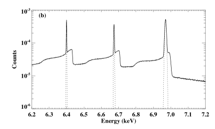
Figure 5: Simulated profiles of Compton scattered Fe K$\alpha$ lines in the accretion column of an mCV with (a) $\mbox{$M_{\rm wd}$}=1.0\,\mbox{$M_{\sun}$}$ and (b) $\mbox{$M_{\rm wd}$}=0.5\,\mbox{$M_{\sun}$}$. In both cases the inclination angle is $i=90^{\scriptscriptstyle{\circ}}$, the specific mass accretion rate is $\dot{m}=10~{}\mbox{$\rm g\,cm^{-2}\,s^{-1}$}$ and the ratio of cyclotron to bremsstrahlung cooling at the shock is $\epsilon_{\rm s}=10$. The dotted curves show the contribution to each line profile by thermal Doppler broadening only.

Figure 5 shows the profiles of Fe K$\alpha$ lines emitted from mCVs with $\mbox{$M_{\rm wd}$}=1.0\,\mbox{$M_{\sun}$}$ and $\mbox{$M_{\rm wd}$}=0.5\,\mbox{$M_{\sun}$}$ where $i=90^{\scriptscriptstyle{\circ}}$, $\dot{m}=10~{}\mbox{$\rm g\,cm^{-2}\,s^{-1}$}$ and the ratio of cyclotron to bremsstrahlung cooling at the shock is $\epsilon_{\rm s}=10$. Also plotted is the thermal Doppler broadened line profile before scattering (dotted curve). The additional cooling of the plasma in the post-shock flow enhances the density and results in larger scattering optical depths. Because the electron temperature of the shock-heated region decreases as $\epsilon_{\rm s}$ increases, the peak emissivities of the 6.675 keV and 6.97 keV Fe lines are found at larger values of $\zeta$, as can be seen in Fig. 2, which shows the temperature, density and velocity profiles for different cases of $\epsilon_{\rm s}$. The additional cyclotron cooling results in a decrease in the electron temperature and bulk velocity in the post-shock column at a fixed $\zeta$.

For $\epsilon_{\rm s}=10$, the 6.4, 6.675 and 6.97 keV lines are emitted from heights above the WD surface of $x\approx$ 0, $3.1\times 10^{5}$ and $2.4\times 10^{7}$ cm for $\mbox{$M_{\rm wd}$}=0.5\,\mbox{$M_{\sun}$}$, and $x\approx$ 0, 0 and $5.3\times 10^{7}$ cm for $\mbox{$M_{\rm wd}$}=1.0\,\mbox{$M_{\sun}$}$, respectively (Wu et al., 2001). The emission height of the 6.97 keV line is significantly higher than in the $\epsilon_{\rm s}=0$ case and consequently, thermal Doppler broadening is more prominent. The additional cooling in the accretion column also results in a lower plasma temperature at the base of the column, $\zeta=0$ (see Fig. 2), near where irradiation of neutral iron occurs and the fluorescent 6.4 keV line is emitted. This line thus undergoes less thermal Doppler broadening than in the $\epsilon_{\rm s}=0$ case. As a result of Compton scattering, the line profiles show additional broadening and recoil tails redward of the line centre (Fig. 5b). Upscattering features are also evident in the 6.4 and 6.675 keV lines especially for $\mbox{$M_{\rm wd}$}=1.0\,\mbox{$M_{\sun}$}$ (Fig. 5a).

Overall, Compton scattering features are more prominent for cyclotron cooling dominated accretion columns, especially for high accretion rates. For photons viewed at $i=90^{\scriptscriptstyle{\circ}}$, upscattering and recoil features that are only marginally seen in the $\epsilon_{\rm s}=0$ case are considerably more pronounced in the $\epsilon=10$ case. Thus, we expect Compton scattering features to be most conspicuous in Fe K$\alpha$ lines emitted in strongly magnetized mCVs accreting at a high rate.

3.3 Effect of Accretion Column Radius

Figure 6: Simulated profiles of Compton scattered Fe K$\alpha$ lines in an accretion column of an mCV with (a) $\mbox{$M_{\rm wd}$}=1.0\,\mbox{$M_{\sun}$}$ and (b) $\mbox{$M_{\rm wd}$}=0.5\,\mbox{$M_{\sun}$}$ both with a specific mass accretion rate of $\dot{m}=10~{}\mbox{$\rm g\,cm^{-2}\,s^{-1}$}$, a ratio of cyclotron to bremsstrahlung cooling of $\epsilon_{\rm s}=10$, an inclination angle of $i=90^{\scriptscriptstyle{\circ}}$ and accretion column radius of $4.6\times 10^{7}\,\rm cm$ . The dotted curves show the profiles when the column radius is fixed at $0.1\mbox{$R_{\rm wd}$}$ (equivalent to the profiles shown in Fig.5).

The width of the accretion column in mCVs is poorly known and may vary significantly from system to system. In the results presented so far, we have fixed the accretion column radius to be $0.1\mbox{$R_{\rm wd}$}$. Here, we investigate the effect of relaxing this assumption. Figure 6 shows the resulting profiles of Fe K$\alpha$ lines emitted from two mCVs of different masses ($\mbox{$M_{\rm wd}$}=1.0\,\mbox{$M_{\sun}$}$ and $\mbox{$M_{\rm wd}$}=0.5\,\mbox{$M_{\sun}$}$) but with the same absolute accretion column radius of $4.6\times 10^{7}\,\rm cm$. This corresponds to $0.08\mbox{$R_{\rm wd}$}$ for the $1.0\,\mbox{$M_{\sun}$}$ case (Fig. 6a) and $0.05\mbox{$R_{\rm wd}$}$ for the $0.5\,\mbox{$M_{\sun}$}$ case (Fig. 6b). The other parameters used to produce the profiles are the same as those used for Fig. 5, namely $\dot{m}=10~{}\mbox{$\rm g\,cm^{-2}\,s^{-1}$}$, $\epsilon_{\rm s}=10$ and $i=90^{\scriptscriptstyle{\circ}}$. Fig. 6 shows that the changes in the accretion column width generally result in changes near the base of the line profiles, which is broadened by multiple scatterings. The effect of increasing (decreasing) the width of the accretion column is to increase (decrease) the overall scattering optical depth.

The Thompson optical depth across the base of the accretion column is $\sim 20$ for the $1.0\,\mbox{$M_{\sun}$}$ case (Fig. 6a) and $\sim 40$ for the $0.5\,\mbox{$M_{\sun}$}$ case (Fig. 6b). In comparison, the Thompson optical depth across the column base for the same lines when the column has a width of $0.1\mbox{$R_{\rm wd}$}$ (dotted curves in Fig. 6) are $\sim 25$ for $\mbox{$M_{\rm wd}$}=1.0\,\mbox{$M_{\sun}$}$ and $\sim 80$ for $\mbox{$M_{\rm wd}$}=0.5\,\mbox{$M_{\sun}$}$. Fig. 6 indicates that due to the nonlinear nature of multiple scatterings in the accretion column, particularly near the base, small changes in optical depth associated with the accretion column geometry can result in significant changes in line profiles. These changes mostly effect the base of the line profiles.

3.4 Emissivity Profile Effects

Figure 7: Simulated profiles of 6.675 keV and 6.97 keV Fe lines in an mCV accretion column with $\mbox{$M_{\rm wd}$}=1.0\,\mbox{$M_{\sun}$}$, a specific mass accretion rate of $\dot{m}=1~{}\mbox{$\rm g\,cm^{-2}\,s^{-1}$}$, no cyclotron cooling and viewed at an inclination angle of $i=45^{\scriptscriptstyle{\circ}}$ (solid lines). An emissivity profile is used to disperse the photon injection site over a finite range of heights along the post-shock column. The dotted curves show the corresponding profiles for photons injected at a single height where the emissivity peaks for the same mCV parameters (equivalent to the profiles shown in Fig 3a, middle panel).

Realistically, the photon source regions are determined by an emissivity profile along the post-shock region of the accretion column. In the results presented so far, all the photons were injected at a single height in the accretion column corresponding to the location of the peak in the emissivity profile, as calculated by Wu et al. (2001). Here, we investigate the effect of spreading the photon injection site over a finite range of heights in the post-shock region according to the calculated emissivity profiles. Only the 6.675 keV and the 6.97 keV line are studied in this manner since much of the fluorescence 6.4 keV yield derives from beneath the column, where X-ray irradiation is strongest so the injection site is always at the base of the column. Figure 7 shows an example of the emissivity profile effect for the 6.675 keV and 6.97 keV Fe K$\alpha$ lines emitted in an mCV with $\mbox{$M_{\rm wd}$}=1.0\,\mbox{$M_{\sun}$}$, $\dot{m}=1~{}\mbox{$\rm g\,cm^{-2}\,s^{-1}$}$, $\epsilon_{\rm s}=0$ and $i=45^{\scriptscriptstyle{\circ}}$. The dotted curves show the corresponding profiles for the case where photons are injected at a single height (where the emissivity peaks) for the same mCV parameters. These profiles are the same as those shown in Fig. 3a for the $i=45^{\scriptscriptstyle{\circ}}$ case (middle panel).

The line profiles calculated using a realistic emissivity profile (solid curves in Fig. 7) show some additional smearing, particularly redward of the line centre, compared to the single injection site case (dotted curves in Fig. 7). This can be attributed to a small fraction of photons now being emitted from regions closer to the shock, where the temperature is $\approx 34\rm\,keV$ and the flow speed is $\approx 1230\rm\,km.s^{-1}$. Thus, these photons are more affected by Doppler effects than other photons emitted from regions further away from the shock. The small smearing redward of the line centre is therefore due to a combination of Doppler shift and thermal broadening. The effect is not prominent because only a small fraction of photons are emitted close to the shock, as predicted by the emissivity profile (Wu et al., 2001). The FWHM for the 6.675 keV and 6.97 keV line is $\approx$ 8 eV and $\approx$ 9 eV respectively. This corresponds to an additional broadening of approximately 25% for the 6.675 keV line and 11% for the 6.97 keV line.

3.5 Comparison with Observations

Figure 8: Fe K$\alpha$ emission lines for the mCV GK Per detected by Chandra/HETGS (bottom) and simulated by our model for a lower and upper white dwarf mass $\mbox{$M_{\rm wd}$}=0.63\,\mbox{$M_{\sun}$}$ (middle) and $\mbox{$M_{\rm wd}$}=1.11\,\mbox{$M_{\sun}$}$ (top) both with a specific mass accretion rate $\dot{m}=10~{}\mbox{$\rm g\,cm^{-2}\,s^{-1}$}$. The simulated spectra have been convolved with the Chandra/HETGS response function. Cyclotron cooling is negligible and we have averaged the simulated lines over all inclination angles in an orbital period. An offset has been added to the simulated plot to allow a comparison between the spectra. See text for further details.

Chandra/HETGS observations of a number of mCVs were reported by Hellier & Mukai (2004). The highest signal-to-noise spectrum was obtained in two observations of the mCV GK Per during its 2002 outburst. This system is classified as an intermediate polar (IP); the WD accretor is thought to have a magnetic field of $\approx 1\,\rm MG$ (Hellier & Mukai, 2004), and a mass of $\mbox{$M_{\rm wd}$}\geq 0.87\pm 0.24\,\mbox{$M_{\sun}$}$ (Morales Rueda et al., 2002). Its typical X-ray luminosity in the $0.17-15$ keV bandpass is $L_{\rm x}\approx 7.14\times 10^{33}\,\rm erg\,s^{-1}$ (Vrielmann et al., 2005), which places a lower limit on the specific mass accretion rate, $\dot{m}\geq 7.3\,\mbox{$\rm g\,cm^{-2}\,s^{-1}$}$ (adopting $\mbox{$R_{\rm wd}$}\approx 6.7\times 10^{8}\,\rm cm$, inferred using the Nauenberg (1972) mass-radius relation, and assuming that accretion proceeds onto a fraction $\approx 10^{-3}$ of the WD surface area; see e.g. Frank, King & Raine 2002).

Here we present a pilot study of GK Per and produce a simple comparison between the profiles of the simulated and observed spectra. A more detailed analysis of the data is left for future study. The summed first-order HETGS spectrum from the 2002 Chandra observations of GK Per is shown in Figure 8. The He-like and fluorescence Fe K$\alpha$ lines are detected, and there is a possible excess at the expected energy for the H-like line at 6.97 keV. Also shown in Fig. 8 are the upper and lower mass simulated HETGS spectra from a 10 ks Chandra observation of an mCV with parameters appropriate for GK Per: an upper mass of $\mbox{$M_{\rm wd}$}=1.11\,\mbox{$M_{\sun}$}$ with $\mbox{$R_{\rm wd}$}=5\times 10^{8}\,\rm cm$, a lower mass of $\mbox{$M_{\rm wd}$}=0.63\,\mbox{$M_{\sun}$}$ with $\mbox{$R_{\rm wd}$}=8.2\times 10^{8}\,\rm cm$ and for both masses $\dot{m}=10\,\mbox{$\rm g\,cm^{-2}\,s^{-1}$}$ and $\epsilon_{\rm s}=4\times 10^{-5}$. We adopted inclination angles averaged over an orbital period of GK Per ($50^{\scriptscriptstyle{\circ}}\leq i\leq 90^{\scriptscriptstyle{\circ}}$) (Hellier, Harmer & Bendmore, 2004). We also added a normalized bremsstrahlung continuum with an electron temperature $kT_{\rm e}=11\,\rm keV$ (Vrielmann et al., 2005).

The measured equivalent widths of the 6.4, 6.675 and 6.97 keV lines in the Chandra/HETGS spectra of GK Per are 260, 117 and 80 eV, respectively. The relative strength of the lines in the simulated spectra is fixed by the number of photons used in each simulation and the assumed continuum flux level. We used $10^{8}$ photons for all three lines, so that their relative strengths are comparable. We intend to relax this condition in future work. There is a remarkable similarity between the observed and the simulated spectra for the 6.4 keV line in particular. Realistically, the actual strengths of the 6.675 and 6.97 keV lines depend on the ionisation structure of the flow (Wu et al., 2001), since this determines the emissivity of the lines. The H-like and He-like lines are thus potentially powerful diagnostic tools that can be used to deduce the physical properties of the post-shock accretion column in mCVs. The 6.4 keV line strength, on the other hand, depends on the flux of the illuminating X-rays, which is largest near the WD surface. Fluorescent lines may also be produced in the surface atmospheric region around the accretion column (Hellier & Mukai, 2004), and this may contribute to the observed equivalent width of the 6.4 keV line.

The observed fluorescent line in GK Per exhibits a red wing extending to 6.33 keV which Hellier & Mukai (2004) attribute to Doppler shifts. In general we find that bulk Doppler shifts have a negligible effect on Fe K$\alpha$ lines. Our simulated spectra show a weaker red wing arising from downscatterings near the base of the accretion column. The observed spectrum also exhibits a shoulder extending 170 eV redward of the 6.4 keV line centre, which Hellier & Mukai (2004) suggest may be due to Compton downscattering. Our simulations confirm that recoil can indeed affect the fluorescent line when it is emitted at the base of the accretion column, although in our spectra (Fig. 8) there is no clear evidence that recoil extends down to 170 eV redward of the 6.4 keV line.

4 Summary and Conclusion

We have investigated line distortion and broadening effects due to Compton scattering in the accretion column of mCVs using a nonlinear Monte Carlo technique that takes into account the nonuniform temperature, velocity and density profiles of the post-shock column. Scattered Fe K$\alpha$ lines were simulated for a range of different physical parameters: white dwarf mass, accretion rate, magnetic field strength and inclination angle. The photon source regions in the post-shock flow were determined from the ionization structure and the effects due to the bulk velocity Doppler shift and thermal broadening are also considered.

We find that line profiles are most affected by Compton scattering in the cases of low white dwarf mass, high specific mass accretion rate, strong cyclotron cooling and oblique inclination angles. Both a lower white dwarf mass (or equivalently a larger white dwarf radius) and a higher accretion rate result in a higher optical depth, hence more pronounced scattering effects. Strong cyclotron cooling associated with a high magnetic field strength results in a higher density in the post-shock flow and hence, a correspondingly larger optical depth. Recoil signatures are evident for oblique viewing angles when cyclotron cooling becomes important. These are due to scatterings near the base of the flow, where both the dynamical and thermal velocities are small. Sharp upscattering features are also seen in the line profiles for large viewing angles. These upscattering features are attributed to head-on collisions with hot electrons near the shock. Photons emitted close to the shock in the accretion column display more thermal Doppler broadening. This is generally the case for the Fe XXVI 6.97 keV line. The Fe 6.4 keV and Fe XXV 6.675 keV lines are generally emitted at or near the base of the accretion column respectively, and show a relatively small amount of thermal Doppler broadening. Bulk velocity induced Doppler shifts are negligible compared with scattering.

We also investigated the effects of dispersing the 6.675 and 6.97 keV line photons using an emissivity calculated self-consistently from the ionization structure of the post-shock column. We find that, compared to injecting the line photons at a single height where the emissivity peaks, using an emissivity profile does not significantly change the overall profiles of the 6.675 and 6.97 keV lines. The resulting line profiles show a small degree of smearing redward of the line center due to additional dynamical and thermal Doppler effects associated with a small fraction of line photons emitted close to the shock. The effect is most important for the 6.675 keV line. We estimate a fractional increase in the FWHM of no more than $\approx$ 25%.

In general, our simulations predict that recoil in scattering with cool electrons near the base of the column as well as upscattering by hot electrons near the shock can imprint signatures on the profile of lines emitted near the base of the flow. Such Compton signatures may thus be used to determine the primary source region of the fluorescent line. We predict that when 6.4 keV photons are emitted in the dense, cool plasma at the base of the accretion column, they can suffer strong downscattering when propagating through the electrons streaming downward in the flow. The scattering probability is governed by the effective scattering optical depth, which increases with the mass accretion rate of the system.

We convolved simulations with the Chandra response function and compared them to Chandra/HETGS observations of GK Per. Our results indicate that the red wing seen in the 6.4 keV line in GK Per could be attributed to Compton recoil near the base of the flow.

Finally we remark that tighter constraints on the dynamics and flow geometry in magnetized accreting compact objects can be obtained by considering the polarization properties of the lines (see Sunyaev & Titarchuk, 1985; Matt, 2004). There is currently considerable effort to develop X-ray polarimeters which can detect degrees of polarization of the order of one percent (Costa et al., 2001). The spectral resolution of these detectors should be adequate to search for different polarization degrees in emission iron lines. It is possible to include a polarization treatment in our calculations, but the computational algorithm in our Monte Carlo code will need to be revised, which we leave for a future study.

Appendix A The width of the Compton shoulder

Here, we derive an estimate for the width of the prominent wings near the base of the line profiles. Let the accretion flow be along the $z$-axis and consider an observer on the $x-z$ plane. Let $i$ be the line-of-sight inclination angle of the accretion column, and let $\beta$ be the local velocity of the flow, normalized to the speed of light $c$, which can expressed as

$$\vec{\beta} = -\beta\ {\hat{z}}\ .$$

The normalized vector of a scattered photon of energy $E^{\prime}$ propagating in the direction to the observer is

$${\hat{k}}^{\prime} = \sin i\ {\hat{x}}\ +\ \cos i\ {\hat{z}}\ .$$

Suppose that the normalized vector of the incident photon, with energy $E$, is

$${\hat{k}} = \sin\theta\cos\phi\ {\hat{x}}\ +\ \sin\theta\sin\phi\ {\hat{y}}\ +\ \cos\theta\ {\hat{z}}\ .$$

Then the change in energy of the photon, after scattering with an electron in the flow, due to bulk motion is given by

$$\frac{E^{\prime}}{E} = \frac{1-\mu\beta}{(1-{\mu}^{\prime}\beta)+\frac{E}{\gamma m_{\rm e}c^{2}}(1-{\hat{k}}\cdot{\hat{k}}^{\prime})}\ ,$$

where $\gamma=(1-\beta^{2})^{-1/2}$, $\mu\beta={\hat{k}}\cdot{\vec{\beta}}$, and ${\mu}^{\prime}\beta={\hat{k}}^{\prime}\cdot{\vec{\beta}}$ . In terms of the viewing inclination angle and the photon propagation vectors,

$$\frac{E^{\prime}}{E} = \frac{1+\beta\cos\theta}{(1+\beta\cos i)+\frac{E}{\gamma m_{\rm e}c^{2}}(1-\sin i\sin\theta\cos\phi-\cos i\cos\theta)}\ .$$

Then for $\beta\ll 1$ and $E\ll m_{\rm e}c^{2}$,

$$\frac{E^{\prime}}{E} \approx 1+\beta(\cos\theta-\cos i)-\lambda(1-\sin i\sin\theta\cos\phi-\cos i\cos\theta)\ .$$

It follows that

$$\frac{\Delta E}{E} \approx \beta(\cos\theta-\cos i)-\lambda(1-\sin i\sin\theta\cos\phi-\cos i\cos\theta)\ ,$$

where $\Delta E=E^{\prime}-E$ and $\lambda=E/m_{\rm e}c^{2}$.

The maximum energy downshift is caused by the recoil process when the photons are scattered by “cold” electrons (with $\beta\approx 0$). This occurs when $\phi=\pi$, $\theta=\pi-i$, which yields

$$\frac{\Delta E}{E}\bigg{|}_{\rm max~{}down} = -2\lambda\ .$$

This result is practically independent of the WD mass and the viewing inclination angle. For the 6.4 keV line, $\Delta E/E|_{\rm max~{}down}\approx-2.50\times 10^{-2}$.

The maximum energy upshift is caused by a Doppler shift when the photons are scattered by the fastest available downstream electrons (i.e. $\beta$ is no longer a negligible factor). The condition for its occurrence can be derived as follows. Set

$$\frac{\partial}{\partial\phi}\left(\frac{\Delta E}{E}\right) = 0\ ,$$

which gives two conditions for extrema with respect to the azimuthal coordinate: $\phi=0$ and $\phi=\pi$, corresponding respectively to

$$\frac{\Delta E}{E} = \beta(\cos\theta-\cos i)-\lambda(1\mp\sin i\sin\theta-\cos i\cos\theta)\ .$$

Differentiating the above expression with respect to $\theta$ and setting the resulting expression to zero yields the following condition for the extrema:

$$\frac{\sin\theta}{\cos\theta} = \pm\xi\ ,$$

where

$$\xi = \frac{\lambda\sin i}{\beta+\lambda\cos i}\ .$$

The first case ($\phi=0$) leads to a maximum energy upshift, which requires

$$\sin\theta = \frac{1}{\sqrt{1+\xi^{2}}}\ ;$$

$$\ \cos\theta = \frac{\xi}{\sqrt{1+\xi^{2}}}\ .$$

At the viewing inclination angle $i=\pi/2$,

$$\sin\theta = \frac{\beta}{\sqrt{\beta^{2}+\lambda^{2}}}\ ;$$

$$\cos\theta = \frac{\lambda}{\sqrt{\beta^{2}+\lambda^{2}}}\ .$$

Hence, the maximum energy upshift is given by

$$\frac{\Delta E}{E}\bigg{|}_{\rm max~{}up} \approx \sqrt{\beta^{2}+\lambda^{2}}-\lambda\ .$$

If we assume that the maximum $\beta$ takes the free-fall velocity at the WD surface, then $\beta$ is simply the reciprocal of the square root of the WD radius in the Schwarzschild unit, i.e. $\beta=\sqrt{2GM_{\rm wd}/R_{\rm wd}c^{2}}$. For $\mbox{$M_{\rm wd}$}=1.0\,\mbox{$M_{\sun}$}$, $\beta=2.31\times 10^{-2}$, and for $\mbox{$M_{\rm wd}$}=0.5\,\mbox{$M_{\sun}$}$, $\beta=1.23\times 10^{-2}$ (assuming the Nauenberg mass-radius relation (Nauenberg, 1972)), this gives $\Delta E/E|_{\rm max~{}up}\approx 1.36\times 10^{-2}$ and $5.06\times 10^{-3}$ respectively for the 6.4 keV line.

The Compton shoulder of an Fe line is due to a single scattering event. For the 6.4 keV line, the broadening extends over $6.24\rm\,keV\leq E\leq 6.49\rm\,keV$ for a 1.0 $M_{\sun}$ WD and $6.24\rm\,keV\leq E\leq 6.43\rm\,keV$ for a 0.5 $M_{\sun}$ WD (omitting thermal broadening and flow Doppler broadening), when viewed at $i=\pi/2$.

References

- Costa et al. (2001) Costa, E., Soffitta P., Bellazzini R., Brez, A., Lumb, N. & Spandre, G. 2001, Nature, 411, 662
- Cropper (1990) Cropper, M. 1990, Sp. Sci. Rev., 54, 195
- Cropper et al. (2000) Cropper, M., Wu, K. & Ramsay, G. 2000, NewAR, 44, 57
- Cullen (2001a) Cullen, J.G. 2001a, PhD Thesis, University of Sydney
- Cullen (2001b) Cullen, J.G. 2001b, JCoPh, 173, 175
- Frank, King & Raine (2002) Frank, J., King, A. & Raine, D. 2002, Accretion Power in Astrophysics, Cambridge: Cambridge University Press
- Hellier et al. (1998) Hellier, C., Mukai, K. & Osborne, J. P. 1998, MNRAS, 297, 256
- Hellier & Mukai (2004) Hellier, C. & Mukai, K. 2004, MNRAS, 352, 1037
- Hellier, Harmer & Bendmore (2004) Hellier, C., Harmer, S. & Bendmore, A.P. 2004, MNRAS, 349, 710
- King & Lasota (1979) King, A.R., Lasota, J.P., 1979, MNRAS, 188, 653
- Kuncic et al. (2005) Kuncic, Z., Wu, K. & Cullen, J. 2005, PASA, 22, 56
- Lamb & Masters (1979) Lamb, D.Q. & Masters, A.R. 1979, ApJ, 234, L117
- Matt (2004) Matt, G. 2004, A&A, 423, 495
- Morales Rueda et al. (2002) Morales Rueda, L., Still, M.D., Roche, P., Wood, J.H. & Lockley, J.J. 2002, MNRAS, 329, 597
- Nauenberg (1972) Nauenberg M. 1972, ApJ, 175, 417
- Pozdnyakov et al. (1983) Pozdnyakov, L.A., Sobol, I.M., & Sunyaev, R.A. 1983, ASPRv, 2, 189
- Stern et al. (1995) Stern, B., Begelman, M., Sikora, M. & Svensson, R. 1995, MNRAS, 272, 291
- Sunyaev & Titarchuk (1985) Sunyaev, R.A. & Titarchuk, L.G. 1985, A&A, 143, 374
- Vrielmann et al. (2005) Vrielmann, S., Ness, J.-U. & Schmitt, J.H.M.M. 2005, A&A, 439, 287
- Warner (1995) Warner, B. 1995, Cataclysmic Variable Stars, Cambridge: Cambridge University Press
- Wu (2000) Wu, K. 2000, SSRv, 93, 611
- Wu et al. (1994) Wu, K., Chanmugam, G. & Shaviv, G. 1994, ApJ, 426, 664
- Wu et al. (2001) Wu, K., Cropper, M. & Ramsay, G. 2001, MNRAS, 327, 208
- Wu et al. (2003) Wu, K., Cropper, M., Ramsay, G., Saxton, C. & Bridge, C. 2003, Chin. J. Astron. Astrophys., 3 (Suppl.), 235