3d Numerical Models of the Chromosphere, Transition Region, and Corona

Abstract

A major goal in solar physics has during the last five decades been to find how energy flux generated in the solar convection zone is transported and dissipated in the outer solar layers. Progress in this field has been slow and painstaking. However, advances in computer hardware and numerical methods, vastly increased observational capabilities and growing physical insight seem finally to be leading towards understanding. Here we present exploratory numerical MHD models that span the entire solar atmosphere from the upper convection zone to the lower corona. These models include non-grey, non-LTE radiative transport in the photosphere and chromosphere, optically thin radiative losses as well as magnetic field-aligned heat conduction in the transition region and corona.

Institute of Theoretical Astrophysics, University of Oslo, Norway

1 Introduction

The notion that chromospheric and coronal heating in some way follow from excess “mechanical” energy flux as a result of convective motions has been clear since the mid-1940’s. Even so, it is only recently that computer power and algorithmic developments have allowed one to even consider taking on the daunting task of modeling the entire system from convection zone to corona in a single model.

Several of these challenges were met during the last few years in the work of Gudiksen & Nordlund (Gudiksen & Nordlund (2002)), where it was shown that it is possible to model the photosphere to corona system. In their model a scaled down longitudinal magnetic field taken from an SOHO/MDI magnetogram of an active region is used to produce a potential magnetic field in the computational domain that covers 50$\times$50$\times$30 Mm³. This magnetic field is subjected to a parameterization of horizontal photospheric flow based on observations and, at smaller scales, on numerical convection simulations as a driver at the lower boundary.

In this paper we will consider a similar model, but one which simulates a smaller region of the Sun; at a higher resolution and in which convection is included. The smaller geometrical region implies that several coronal phenomena cannot be modeled. On the other hand the greater resolution and the inclusion of convection (and the associated non-grey radiative transfer) should allow the model described here to give a somewhat more satisfactory description of the chromosphere and, perhaps, the transition region and lower corona.

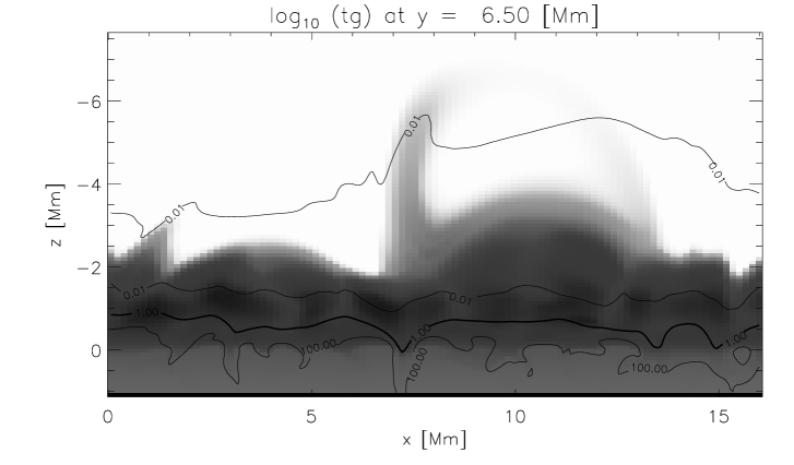
Figure 1.: Temperature structure in one plane of the simulation box. At $z=0$ Mm temperatures span 5000 K to $10\,000$ K, at the bottom of the computational domain, $1.5$ Mm into the convection zone, we find temperatures ranging from $15\,700$ K in down-flowing plumes to $16\,500$ in the gas flowing into the simulation domain. Above the photosphere, the chromosphere extends 2–4 Mm (see also Figure 4) with temperatures from 2000 K to 8000 K. The upper 10 Mm of the model is filled with plasma at transition region and coronal temperatures of up to some 1 MK, though even at great heights there are intrusions of cooler gas. Also plotted are contours of plasma $\beta=p_{g}/p_{B}$; $\beta=1$ is found in the mid to lower chromosphere, occasionally almost reaching the photosphere. $\beta$ is much greater than one in the convection zone, much smaller than one in the transtion region and corona. Note that we find high intensity “bright points” in the photosphere where the magnetic field is strong. High intensity in the chromosphere is due both hydrodynamic shocks and magnetic heating.

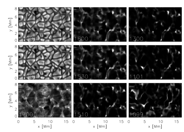
Figure 2.: Emergent intensities in various continua (wavelength in Å in each panel) as seen from above. The continua at 5000 and 3000 Å show photospheric granulation, the continuum at 1700 is formed a few hunderd kilometers higher and shows reverse granulation, at 1600 and 1530 Å we sample the the upper photosphere. The 1510 continuum is just shortward of the bound-free edge of neutral silicon, carrying the formation to the lower chromosphere. The 1300 and 1101 continua are formed in the lower-mid chromosphere and the 1099 continuum is just shortward of the bound-free edge of neutral carbon and is formed in the upper chromosphere.

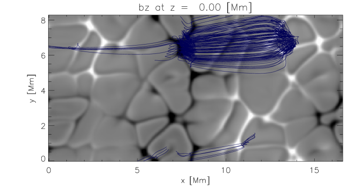
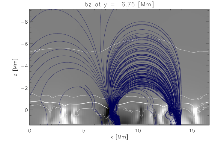
Figure 3.: The ${\mathbf{B}}_{z}$ component of the magnetic field in the photosphere, $z=0$ Mm is shown in the upper panel. A subset of magnetic field lines – a semi-random selection based on the strongest magnetic field at the height where $\beta\approx 1$ is drawn. The lower panel shows the same, projected from side. In addition countours of constant $\beta$ are drawn in white. Note that the field lines identified fit well with the location of maximum emission in the Ne viii and Mg X lines as evident in Figure 6.

2 Method

There are several reasons that the attempt to construct forward models of the convection zone or photosphere to corona system has been so long in coming. We will mention only a few:

The magnetic field will tend to reach heights of approximately the same as the distance between the sources of the field. Thus if one wishes to model the corona to a height of, say, 10 Mm this requires a horizontal size close to the double, or 20 Mm in order to form closed field regions up to the upper boundary. On the other hand, resolving photospheric scale heights of 100 km or smaller and transition region scales of some few tens of kilometers will require minimum grid sizes of less than 50 km, preferably smaller. (Numerical “tricks” can perhaps ease some of this difficulty, but will not help by much more than a factor two). Putting these requirements together means that it is difficult to get away with computational domains of much less than 150³ — a non-trivial exercise even on todays systems.

The “Courant condition” for a diffusive operator such as that describing thermal conduction scales with the grid size $\Delta z^{2}$ instead of with $\Delta z$ for the magneto-hydrodynamic operator. This severely limits the time step $\Delta t$ the code can be stably run at. One solution is to vary the magnitude of the coefficient of thermal conduction when needed. Another, used in this work, is to proceed by operator splitting, such that the operator advancing the variables in time is $L=L_{\rm hydro}+L_{\rm conduction}$, then solving the conduction operator implicitly, for example using the multigrid method.

Radiative losses from the photosphere and chromosphere are optically thick and require the solution of the transport equation. A sophisticated treatment of this difficult problem was devised by (Nordlund 1982) in which opacities are binned according to their magnitude; in effect one is constructing wavelength bins that represent stronger and weaker lines and the continuum so that radiation in all atmospheric regions is treated to a certain approximation. If one further assumes that opacities are in LTE the radiation from the photosphere can be modeled. Modeling the chromosphere requires that the scattering of photons is treated with greater care (Skartlien (2000)), or in addition that one uses methods assuming that chromospheric radiation can be tabulated as a function of local thermodynamic variables a priori.

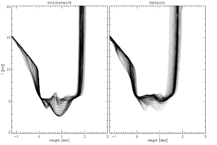
Figure 4.: Temperature structure in the chromosphere as found above a region of very weak photospheric field (left panel) and above a region of stronger magnetic field (right panel). Note that the average chromospheric temperature is higher and that the transition region extends further down towards the photosphere in the ‘network’. Note also the evidence of shock propagation in the left ‘internetwork’ panel.

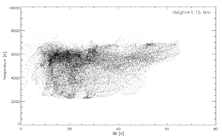
Figure 5.: Relation between the magnetic field strength and temperature in the chromosphere 1.15 Mm above the photosphere.

In this paper we have used the methods mentioned to solve the MHD equations, including thermal conduction and non-grey non-LTE radiative transfer. The numerical scheme used is an extended version of the numerical code described in Dorch & Nordlund (1998); Mackay & Galsgaard (2001) and in more detail by Nordlund & Galsgaard at http://www.astro.ku.dk/$\sim$kg. In short, the code functions as follows: The variables are represented on staggered meshes, such that the density $\rho$ and the internal energy $e$ are volume centered, the magnetic field components ${\bf B}$ and the momentum densities $\rho{\bf u}$ are face centered, while the electric field ${\bf E}$ and the current ${\bf J}$ are edge centered. A sixth order accurate method involving the three nearest neighbor points on each side is used for determining the partial spatial derivatives. In the cases where variables are needed at positions other than their defined positions a fifth order interpolation scheme is used. The equations are stepped forward in time using the explicit 3rd order predictor-corrector procedure by Hyman (1979), modified for variable time steps. In order to suppress numerical noise, high-order artificial diffusion is added both in the forms of a viscosity and in the form of a magnetic diffusivity.

3 3d Models

The models described here are run on a box of dimension 16$\times$8$\times$16 Mm³ resolved on a grid of $256\times 128\times 160$ points, equidistant in $x$ and $y$ but with increasing grid size with height in the $z$ direction. At this resolution the model has been run a few minutes solar time starting from an earlier simulation with half the resolution presented here. The lower resolution simulation had run some 20 minutes solar time, starting from a (partially) relaxed convective atmosphere in which a potential field with field strengths of order 1 kG at the lower boundary and an average unsigned field strength of 100 G in the photosphere was added. The convective atmosphere has been built up from successively larger models, and has run of order an hour solar time; some periodicities are still apparent at lower heights where the time scales are longer (of order several hours near the lower boundary).

The initial potential magnetic field was designed to have properties similar to those observed in the solar photosphere. The average temperature at the bottom boundary is maintained by setting the entropy of the fluid entering through the bottom boundary. The bottom boundary, based on characteristic extrapolation, is otherwise open, allowing fluid to enter and leave the computational domain as required. The magnetic field at the lower boundary is advected with the fluid. As the simulation progresses the field is advected with the fluid flow in the convection zone and photosphere and individual field lines quickly attain quite complex paths throughout the model.

A vertical cut of the temperature structure in the model is shown in Figure 1. In Figure 2 we show the emergent intensity in various continua as calculated a posteriori from a data cube some minutes into the simulation run. Though the analysis of these intensities is far from complete (the model is still in some need of further relaxation) a number of observed solar characteristics are recognized. Solar granulation seems faithfully reproduced in the 300 nm and 500 nm bands including bright patches/points in intergranular lanes where the magnetic field is strong. Reverse granulation is evident in the 170 nm band as is enhanced emission where the magnetic field is strong. Bright emission in the bands formed higher in the chromosphere is a result of both strong magnetic fields as well as hydrodynamic shocks propagating through the chromosphere.

The field in the models described here was originally potential. However, it is rapidly deformed by convective motions in the photosphere and below and becomes concentrated in down-flowing granulation plumes on a granulation time-scale. In regions below where $\beta\equiv{p_{g}/p_{B}}=1$ the magnetic field is at the mercy of plasma motions, above the field expands, attempts to fill all space, and forms loop like structures. The $B_{z}$ component of the magnetic field in the photosphere is shown in the upper panel of Figure 3, also plotted are magnetic field lines chosen on the basis of their strength at the surface where $\beta=1$. The same field lines seen from the side are plotted in the lower panel of Figure 3 overplotted the vertical magnetic field $B_{z}$.

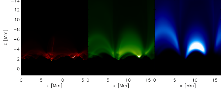
Figure 6.: Line emission from the O vi, 300 kK formation temperature, Ne viii line, formed at roughly 700 kK, and Mg x formed at some 1 MKk, all seen seen from the side. Note the ray of O vi emission near $x=7$ Mm that extends to some $z=-6$ Mm.

Chromospheric energetics and dynamics are set by a number of factors. Among the most important of these are acoustic waves generated in the photosphere and convection zone impinging on the chromosphere from below; the topology of the magnetic field and the location of the plasma $\beta=1$ surface; the amount of chromospheric heating due the dissipation of magnetic energy; non-LTE radiative losses and related phenomena such as time dependent ionization and recombination. Most of these phenomena with the exception of time dependent ionization is accounted for (to various degrees of accuracy) in the models presented here. The latter is currently under implementation (Leenaarts et al. (2007)). Examples of the chromospheric temperature structure and its relation to the magnetic field are shown in Figures 4 and 5.

As the stresses in the coronal field grow so does the energy density of the field. This energy must eventually be dissipated; at a rate commensurate with the rate at which energy flux is pumped in. This will depend on the strength of the magnetic field and on the amplitude of convective forcing. On the Sun the magnetic diffusivity $\eta$ is very small and gradients must become very large before dissipation occurs; in the models presented here we operate with an $\eta$ many orders of magnitude larger than on the Sun and dissipation starts at much smaller magnetic field gradients. Even so, it seems the model is able to reproduce diagnostics that resemble those observed in the solar transition region and corona as shown in Figure 6. (It is also interesting to note that we find emission from O vi 103.7 nm in a narrow ray up to 6 Mm above the photosphere, much higher than it should be found in a hydrostatically stratified model.)

4 Conclusions

The model presented here seems a very promising starting point and tool for achieving an understanding of the outer solar layers. But perhaps a word or two of caution is in order before we celebrate our successes. Are the tests we are subjecting the model to — e.g. the comparison of synthetic observations with actual observations actually capable of separating a correct description of the sun from an incorrect one? Conduction along field lines will naturally make loop like structures. This implies that reproducing TRACE-like “images” is perhaps not so difficult after all, and possible for a wide spectrum of coronal heating models. The transition region diagnostics are a more discerning test, but clearly it is still too early to say that the only possible coronal model has been identified. It will be very interesting to see how these forward coronal heating models stand up in the face of questions such as: How does the corona react to variations in the total field strength, or the total field topology, and what observable diagnostic signatures do these variations cause? One could also wonder about the role of emerging flux in coronal heating: How much new magnetic flux must be brought up from below in order to replenish the dissipation of field heating the chromosphere and corona?

Acknowledgments.

This work was supported by the Research Council of Norway grant 146467/420 and a grant of computing time from the Program for Supercomputing.

References

- Dorch & Nordlund (1998) Dorch S. B. F., Nordlund A., 1998, A&A 338, 329
- Gudiksen & Nordlund (2002) Gudiksen B. V., Nordlund Å., 2002, ApJ 572, L113
- Hyman (1979) Hyman J., 1979, in R. Vichnevetsky, R. Stepleman (eds.), Adv. in Comp. Meth. for PDE’s—III, 313
- Leenaarts et al. (2007) Leenaarts J., Wedemeyer-Böhm S., Carlsson M., Hansteen V. H., 2007, in Coimbra Solar Physics Meeting ion the Physics of Chromospheric Plasmas, ASP Conference Series, Vol. in this volume
- Mackay & Galsgaard (2001) Mackay D. H., Galsgaard K., 2001, Solar Phys. 198, 289
- Nordlund (1982) Nordlund Å., 1982, A&A 107, 1
- Skartlien (2000) Skartlien R., 2000, ApJ 536, 465