Connecting microscopic simulations with kinetically constrained models of glasses

Abstract

Kinetically constrained spin models are known to exhibit dynamical behavior mimicking that of glass forming systems. They are often understood as coarse-grained models of glass formers, in terms of some “mobility” field. The identity of this “mobility” field has remained elusive due to the lack of coarse-graining procedures to obtain these models from a more microscopic point of view. Here we exhibit a scheme to map the dynamics of a two-dimensional soft disc glass former onto a kinetically constrained spin model, providing an attempt at bridging these two approaches.

I Introduction

The origin of the onset of ultra-slow dynamics in glassy systems, and in particular, glass-forming liquids, remains a murky subject, with many competing ideas and tantalizing clues as to underlying causes, despite years of effort by a large community of researchers Classic . Recently it has become increasingly clear that dynamical heterogeneities, regions of atypically fast dynamics that are localized in space and time, are intimately connected to the phenomenon of glassiness Sillescu ; Ediger ; Glotzer ; Richert ; Castillo , becoming increasingly important at lower temperature scales towards and below the glass transition temperature $T_{g}$ DHexp ; Kob ; Donati1 ; Donati2 .

Early ideas about heterogeneous dynamics focused on the idea of co-operatively rearranging regions which grow with decreasing temperature Adam . Currently, molecular dynamics (MD) simulations of supercooled liquids allow much greater access to the microscopic details of this heterogeneity HarrowellDH ; Yamamoto ; Andersen . This has included the observation of “caging” of particles, and string-like excitations that allow particles to escape these cages Donati1 ; Perera2 ; Gebremichael1 ; Stevenson , which has been confirmed in experiments on colloidal glasses Kegel-Weeks . However, MD simulations have the drawback that it is difficult to reach the low temperatures and long times characteristic of the glassy phase.

An alternative approach to reach low temperatures and long times, but without a microscopic foundation, is to study simple models of glassiness, kinetically constrained models (KCMs) Ritort ; FA ; Graham ; CG ; PNAS ; LMSBG , such as the Fredrickson-Andersen (FA) model FA or the East model Evans , or variations such as the North-East model PNAS , which mimic the constrained dynamics of real glassy systems but have trivial thermodynamics. These may be viewed as effective models for glasses, in terms of some coarse-grained degree of freedom often labelled “spins”, also termed a “mobility field” by some authors PNAS . In Fredrickson and Andersen’s original work, they posited that the degrees of freedom may be high and low density regions, related to earlier suggestions by Angell and Rao ARao . Despite these appealing physical pictures, it has not been particularly clear to what physical quantity this “mobility field” corresponds. If KCMs are truly effective models of glassy behavior then it should be possible to make a connection between some set of degrees of freedom, in a MD simulation, for instance, and a KCM.

In this paper we propose a specific coarse-graining procedure to explore whether a link can be made between MD simulations and KCMs of glassiness. Previous work in this direction found evidence of dynamic facilitation in MD simulations Donati2 ; Vogel , however, there was no attempt to map the dynamic facilitation onto a KCM. We use an approach directly related to the idea of a “mobility” field, using the local mean-square displacement (MSD) in a suitably defined box to define a spin variable. Regions with large average MSD correspond to “up” spins and those with low average MSD correspond to “down” spins. We give specific details of our procedure below.

We investigate the time and length-scale dependence of this coarse-graining. The two characteristic time scales are the beta relaxation time scale, $t_{\beta}$ (corresponding physically to the time for relaxation within a cage) and the longer alpha relaxation time scale, $t_{\alpha}$, which corresponds to the time-scale on which structural relaxation of cages occurs. We find that evidence of dynamic facilitation becomes much stronger at longer times of order $t_{\alpha}$, than at earlier times of order $t_{\beta}$. We also study the effect of changing the size of the coarse-graining box, $l$, in space and consider values $0.02\leq l/L\lesssim 0.25$, where $L$ is the system size. With appropriate choices of time and lengthscales, we find a clear mapping from our MD simulations onto a KCM similar to the 1-spin facilitated FA model. This is not what one might naively expect. Since we study a fragile glass-former, we expect to find a KCM which exhibits super-Arrhenius relaxation, whereas the 1-spin facilitated FA model has Arrhenius relaxation – the super-Arrhenius growth of timescales is absorbed into the coarse graining time, which is most effective at capturing kinetically constrained behaviour when it is of order $t_{\alpha}$ contrary to expectations based on the idea of a mobility field FA ; PNAS .

The demonstration of a coarse-graining procedure to translate from a microscopic model to a coarse-grained KCM for glasses can shed light on the following: it provides a physical interpretation to the “mobility field”; it can give a stronger theoretical justification for the use of KCMs to study glassy dynamics; and may open the door to further exploration of the link between microscopic models and long-time features of dynamics, i.e. answering the question: for a given interparticle interaction potential, how will the dynamics of the glass behave?

This paper is structured as follows: in Sec. II we give details of our molecular dynamics simulations, in Sec. III we describe our coarse-graining procedure and present the results of coarse-graining MD simulations, and then in Sec. IV we discuss our results.

II Molecular Dynamics Simulations

We study the dynamics of a well-characterized glass former: the binary soft disc model with a potential of the form $\epsilon\left(\frac{\sigma_{\alpha\beta}}{r}\right)^{12}$ in two dimensions Perera ; Yamamoto ; Perera2 . This mixture of discs with size ratio 1:1.4 inhibits crystallization upon cooling. We choose a 75:25 ratio of small to large particles and cool the system with the density fixed at $\rho=0.85\sigma_{11}^{-2}$. All temperatures and lengths are quoted in the standard reduced units of the Lennard-Jones potential using the small disc diameter $\sigma_{11}$, as a length scale. This mixture has the same glassy characteristics as the model previously documented in Ref. Perera . Post-equilibration calculations are performed using the recently introduced iso-configurational (IC) ensemble AWC1 . Our results are qualitatively similar if we follow a single trajectory with no IC averaging, but IC averaging gives smoother trends as a function of temperature.

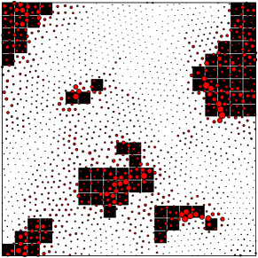
Figure 1: Averaged mean square displacement from IC simulations of length $\tau_{e}$ at $T=0.360$. On this time scale there is movement throughout the cell.Not all of the the larger groups grow into regions of large displacements at longer timescales. We show the corresponding spin configuration, with up spins represented as black squares.

In Fig. 1 we show the MSD for each particle averaged over 500 independent trajectories started from the same particle configuration in a $N=1600$ particle system. Each trajectory is evolved for a time $\tau_{e}$, where $\tau_{e}$ is the time that it takes for the self-intermediate scattering function for the small particles $F_{s}(k,t)=\frac{1}{N}\sum_{i}\left<\sin\left(k\left|r_{i}(t)-r_{i}(0)\right|\right)/\left(k\left|r_{i}(t)-r_{i}(0)\right|\right)\right>$ (note that the form we use has already been averaged over angle) to decay by a factor of $1/e$ – this is roughly $t_{\alpha}$. The $k$ value chosen is that of the first peak of the static structure factor. It is clear that there are regions of much higher MSD than the average, and that these regions are reasonably widely spaced. The important question for mapping the dynamics to a KCM is how such regions influence the behavior of their neighbors.

The MSD in the IC ensemble simulations can be seen as a measurement of the propensity for a particle to move based on the initial configuration. As noted by Widmer-Cooper and Harrowell, each trajectory within the ensemble does not reproduce the same dynamics AWC1 . The final propensity is therefore the composite of a set of trajectories that is determined solely by the initial particle positions. We can follow the change of the propensity in time by following a single trajectory and performing IC simulations separated by a time $\tau_{s}$ (which we mostly take to be $\sim\tau_{e}$). The KCM that we determine is one that is obtained from an IC average over 500 trajectories.

III Coarse graining procedure

There are two parts to our coarse-graining procedure. First, we identify the spins that enter in the KCM (using the results of the MD simulations). Second we infer the dynamics of these spins. Specificly, we construct a model which has a Hamiltonian

$$H=\frac{J}{2}\sum_{i}s_{i},$$ (1)

where $s_{i}$ is a “spin” variable on a site $i\in[1,N_{S}]$ (where $N_{S}$ is the number of sites in the spin model) for which up ($s_{i}=1$) corresponds to an active region and down ($s_{i}=-1$) corresponds to an inactive region, and $J$ is some (yet to be determined) energy scale. The first part of the coarse-graining procedure is to find a way to determine the separation of regions into up and down spins. In general one might also consider terms in the Hamiltonian related to spin-spin interactions LMSBG , but in their simplest forms, KCMs are usually taken to have the form in Eq. (1). This implies that at high temperatures there are no static correlations, as one expects in a liquid. The model Eq. (1) has no interactions and any glassy phenomenology must come from the dynamical rules that govern how spins flip. These dynamical rules are usually stated in the form that the probability of a spin flipping is dependent on the state of its neighbors FA . To be more precise, we can note that Glauber rates for flipping a spin $i$ are given by Ritort ; LMSBG :

$$w_{i}({\mathbf{s}})=f_{i}({\mathbf{s}})\left\{\begin{array}[]{cc}n_{\downarrow},&s_{i}=1\\ n_{\uparrow},&s_{i}=-1\end{array}\right.$$ (4)

which respects detailed balance, and the concentration of up spins (with $n_{\uparrow}+n_{\downarrow}=1$) is

$$n_{\uparrow}=\frac{1}{1+e^{J/T}},$$ (5)

and ${\mathbf{s}}=(s_{1},\ldots,s_{N_{S}})$. We determine the function $f_{i}({\mathbf{s}})$ assuming that it has the form $f(m)$, where $m$ is the number of up spins on sites neighboring site $i$, similarly to the formulation of the FA model FA . We analyze the data from the MD simulations to determine $f(m)$. It is desirable that the results be relatively insensitive to the parameters entering the coarse-graining procedure, which is what we find.

Our coarse-graining procedure to determine spins and sites is as follows: we perform a set of simulations to give $n\simeq 100$ timesteps in the IC ensemble. The timesteps are chosen to be $t_{\beta}$, $0.6\tau_{e}$, and $\tau_{e}$ to check the coarse-graining in time. We find that the fitting form $\tau_{e}=\frac{0.85}{T}e^{\left(\frac{0.5}{T}\right)^{4.5}}$ works well over the entire temperature range we consider ($T=0.36$ to $T=0.96$), although for $T\leq 0.48$ the form $\tau_{e}=0.025e^{\left(\frac{1.1}{T}\right)^{2}}$ works equally well. We take each of the snapshots of IC averaged particle configurations and coarse-grain in space, by dividing the sample into $(l/L)^{2}$ boxes lying on a square lattice footnote , so that each particle is assigned to a box. We take $l$ to be small and fixed to $l=2$ most of the time (this appears to be roughly the length-scale of the cage-breaking process, and also of the order of the dynamic correlation length, $\xi$ Perera ) and assume $l$ to be temperature and time independent. Since we have at most 1600 particles in our system, when we go to large coarse graining lengths ($l\geq 8$), we start to get close to the system size and finite size effects are important, i.e. $l/L\gtrsim 0.2$.

We associate a spin with each box, either up or down depending on whether the MSD per particle in the box is larger or smaller than some cutoff. We adjust the cutoff so that $n_{\uparrow}$ takes its equilibrium value, Eq. (5). This leaves the freedom to choose the energy scale $J$. A seemingly natural energy/temperature scale associated with glassy dynamics appears to be that where the relaxation time for the small particles starts to stretch more quickly and there is a marked onset of dynamic heterogeneity; roughly $T\sim 0.5$. This is also the temperature where the scaling between diffusion and relaxation times changes Perera , motivating us to choose $J=0.5$ (in the same units as $T$). However, we check that our results are robust under varying this choice (see Fig. 2). In general we find that if $J\gtrsim 0.3$ the probabilities of spin flips that we identify are identical.

Now, one of the assumptions that underlies writing down Eq. (1) is that there are no static correlations. Given that the spins we consider are themselves defined through dynamics, albeit within a single coarse-graining time, it is difficult to be certain that one can extract truly static correlations. Nevertheless, we checked for static correlations in the spin model defined above and find that at high temperatures there are no static correlations, whereas for temperatures below about $T=0.45$, there are “static” correlations on a lengthscale of up to two lattice spacings (at $T=0.36$), that appears to be growing with decreasing temperature. This is in accord with the expectation that as the spins diffuse, they lead to local relaxations that appear as a static correlation in a single snapshot, but can be resolved, for example, by the dynamic four-point susceptibility that has been discussed extensively in the literature Dasgupta ; Donati3 ; Doliwa ; FranzParisi ; Glotzer2 ; BB ; Toninelli ; Berthier . It is also possible that extra terms involving spin-spin interactions should perhaps be included in the model as these can also lead to static correlations, but the relatively short correlation length, and the existence of dynamic correlations as discussed above suggests that we can ignore these interactions as a first approximation. We shall proceed under this assumption of non-interacting spins and discuss some consequences of interactions that appear to give small corrections to our non-interacting results.

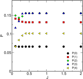
Figure 2: $P(m)$ at $m=$ 0, 1, 2, 3, and 4, for spin flips down to up as $J$ is varied, with a coarse-graining timescale of $\tau_{e}$ at $T=0.36$ with $l=2$.

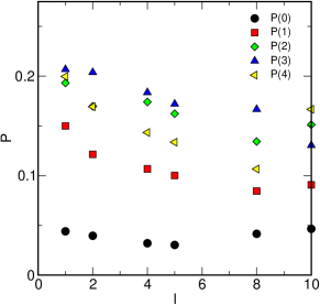
Figure 3: $P(m)$ as a function of $m$ for spin flips up to down as $l$ is varied, with a coarse-graining timescale of $\tau_{e}$ at $T=0.36$ with $J=0.5$.

In Figs. 2 and 3 we show some of our checks on the coarse-graining procedure. All of these are at $T=0.36$. In particular, in Fig. 2 we show how $P(m)$, the probability of a spin flip between consecutive time steps changes with variations in $J$ at fixed $l=2$ and $T$ for spin flips from down to up. [At a fixed temperature, $P(m)\propto f(m)$.] In Fig. 3 we show how $P(m)$ changes with variations in $l$ at fixed $J$ and $T$ for spin flips with up to down. Comparable results are found for the spin flips not shown. Statistical error bars are comparable to the size of the symbols.

We have thus defined our spins. Now we must understand their dynamics. To do this, we ask the question, for an up or down spin with $m$ nearest neighbors that are up spins, what is the probability that it will flip in a given time-step? This is the way that the classic FA model is posed. We display the function $f(m)$ as a function of temperature in Figs. 4 and 5 for coarse graining times of $t_{\beta}$ and $\tau_{e}$ respectively.

In Figs. 4a) and 5a) we consider $m=$ 0, 1, and 2, whilst for clarity, in Figs. 4b) and 5b) we show $m=3$ and $m=4$. The behaviour between these two coarse-graining times is quite distinct. For a coarse-graining time of $t_{\beta}$ there is no strong tendency towards kinetically constrained dynamics, whereas for a coarse graining time of $\tau_{e}$ there are quite strong indications. For a coarse graining time of $\tau_{e}$, at low temperatures ($T\lesssim 0.5$), $f(0)$, $f(1)$ and $f(2)$ are distinctly different, and there is qualitative agreement between $f(m)$ determined from either up to down spin flips or down to up spin flips. Similar results are seen for $f(3)$ and $f(4)$.

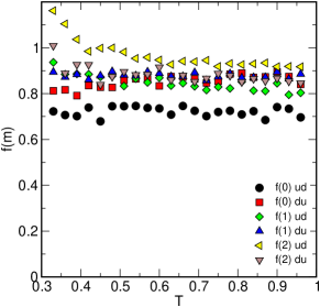
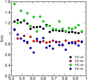
Figure 4: $f(m)$ as a function of temperature from both up to down and down to up spin flips a) m = 0, 1, 2; b) m = 3, 4 with coarse graining time $t_{\beta}$

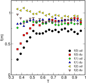
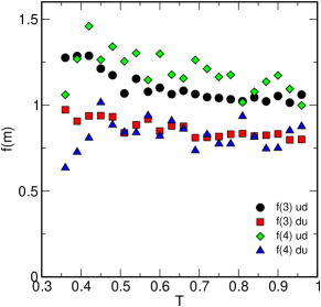
Figure 5: $f(m)$ as a function of temperature from both up to down and down to up spin flips a) m = 0, 1, 2; b) m = 3, 4 with coarse graining time $\tau_{e}$

Detailed balance implies that $f(m)$ determined from either type of spin flip should be the same if the system is described precisely by a model of the type in Eq. (1). In Figs. 4 and 5 there are small but clear differences between $f(m)$ determined from the two types of spin flips. We believe that there are two sources for this discrepancy. Probably most important is the presence of spin-spin interactions which are not accounted for in Eq. (1). Such interactions mean that $f(m)$ does not depend solely on $m$, although at low temperatures it is clear that $m$ is the most important variable controlling the behaviour of $f(m)$. Secondly, the magnitude of the discrepancy between rates varies from temperature to temperature point. This is likely to be from biases that are forced on us by computational restrictions. In principle, one would like to equilibrate a large number of independent particle configurations, then perform an IC average for each initial condition to determine $f(m)$. In practice, it is computationally expensive to equilibrate at low temperatures, so we equilibrate one particle configuration and then use this to generate subsequent particle configurations from one member of the IC ensemble. This introduces a sampling bias that is likely to contribute to the discrepancy between the rates. We note that even for a single trajectory, there are signatures of kinetically constrained dynamics, but cleaner results are obtained from our IC averaging, and we expect averages over more independent particle configurations to yield more precise results. Despite these caveats, Fig. 5 clearly illustrates that the coarse-graining procedure we have devised gives strong evidence of kinetically constrained dynamics, and appears to give a mapping of a microscopic simulation to a KCM.

The signatures of kinetically constrained behavior only start to show up in the coarse grained spin model for $T\lesssim 0.5$. which is around the temperature at which the relaxation time for small particles increases quickly with decreasing temperature, and is also around where the Stokes-Einstein relation breaks down. An important point to note about KCMs is that they are expected to give the best account of glassy dynamics when $n_{\uparrow}\ll 1$. In the temperature range we consider, this is only approximately true, for instance, at $T=0.36$, $n_{\uparrow}\simeq 0.2$ (with $J=0.5$, although for larger $J$, $n_{\uparrow}$ is considerably smaller, and the $f(m)$ we have determined are unchanged). The requirement of a vanishing number of up spins suggests that to extract a specific KCM from our data, one should consider the limit that $T\to 0$. Figure 5 certainly suggests that as $T\to 0$, $f(0)\to 0$, but it is harder to determine the fate of $f(m)$ for $m\neq 0$. However, our results suggest a KCM that might apply in the limit $T\to 0$ defined by (with $\alpha$ constant)

$$f(m)=\left\{\begin{array}[]{cc}0,&m=0\\ \alpha,&m\geq 1.\end{array}\right.$$ (8)

The most important feature of the model that is realised, whether it is exactly as in Eq. (8) or not, is that it is of the one-spin facilitated type Ritort . It appears unlikely from Fig. 5 that $f(1)\to 0$ as $T\to 0$ as would be required for a two-spin facilitated KCM. We have verified with Monte Carlo simulations that this model gives timescales that diverge in an Arrhenius fashion at low temperatures. However, the fact that the timestep in the KCM is also strongly temperature dependent (through $\tau_{e}$) leads to a fragile behaviour of timescales when expressed in terms of the time units of the MD simulations, i.e. $\tau\sim e^{A/T^{2}}$ for some constant $A$.

IV Discussion

There are several goals in trying to map MD simulations of a glass former onto a KCM. The first is making a connection between microscopic particle motions and some effective theory of glassy dynamics. A second is to determine the long-time dynamics of a given glass former at very low temperatures where MD simulations are ineffective, say through Monte Carlo simulations of the KCM, or in some cases, analytic calculations.

The mapping of MD simulations to a KCM that we have achieved is not what one might naively expect. From the discussions in the literature PNAS ; FA , the expectation would be that for coarse-graining on some small lengthscale (as we do), and on a timescale much less than $t_{\alpha}$ or $\tau_{e}$, one obtains a KCM which has within it the physics of the alpha relaxation time. Our attempts along these lines are shown in Fig. 4, which clearly indicates that this expected behaviour does not hold. It is only when one coarse-grains on timescales of order $t_{\alpha}$ that we start to see effective kinetic constraints emerging. In order to get fragile glass like behaviour, as seen in the MD simulations, from the constant coarse-graining time scenario, one would require the KCM obtained from the coarse-graining procedure to be multi-spin facilitated, since single-spin facilitated models of the type found in Eq. (8) are known to have activated dynamics Ritort . This suggests that there may be alternative coarse graining schemes that capture a connection between MD simulations and KCM. Nevertheless, to the best of our knowledge, we have demonstrated the first effective mapping of MD simulations onto a KCM. The “spins” of our model correspond to regions of high or low MSD per particle and hence are in the spirit of the “mobility field”PNAS .

Given that the mapping we exhibit does not allow us to obtain the fragile glass behaviour of the original model from our KCM, it is interesting to ask what physics the spins that we map to are sensitive to. We believe they are sensitive to slow structural relaxation that proceeds on time scales even longer than $t_{\alpha}$. This appears to be consistent with recent work by Szamel and Flenner Szamel that suggests that continuing relaxations beyond $t_{\alpha}$ lead to the timescale for the onset of Fickian diffusion to be an order of magnitude longer than $t_{\alpha}$ and grow faster than $t_{\alpha}$ at low temperatures. The same authors also proposed a non-gaussian parameter which differs from that conventionally used in studies of glass formers Flenner . This non-gaussian parameter has a peak at later times than the conventional one, at timescales of order $t_{\alpha}$, where it appears that heterogeneity in the distribution of particle displacements is maximal. This might be related to why a “spin” definition based on mean square displacement, as we use here, is most sensitive to physics on the timescale of $t_{\alpha}$. This suggests that in order to make a mapping to a KCM more in line with naive expectations, one should use quantities that have maximum contrast on timescales which are considerably shorter than $t_{\alpha}$. Such an approach may be a viable way to construct effective theories of glassy dynamics in this and in other systems. We have demonstrated a particular numerical coarse-graining procedure, and we hope that our results may help point the way to analytic approaches to connect microscopic models of glasses to KCMs, and further insight into the glass problem.

V Acknowledgements

Calculations were performed on Westgrid. The authors thank Horacio Castillo, Claudio Chamon, and Mike Plischke for discussions, and David Reichman for critical comments on the manuscript. The authors also thank the anonymous referees for their comments. This work was supported by NSERC.

References

- (1) T. R. Kirkpatrick and P. G. Wolynes, Phys. Rev. A 35, 3072 (1987); Phys. Rev. B 36, 8552 (1987); T. R. Kirkpatrick and D. Thirumalai, Phys. Rev. Lett. 58, 2091 (1987); C. A. Angell, J. Phys. Cond. Mat. 12, 6463 (2000); G. Tarjus, et al., J. Phys. Cond. Mat. 12, 6497 (2000); P. G. Debenedetti and F. H. Stillinger, Nature 410, 259 (2001).
- (2) H. Sillescu, J. Non-Cryst. Solids 243, 81 (1999).
- (3) M. D. Ediger, Annu. Rev. Phys. Chem. 51, 99 (2000).
- (4) S. C. Glotzer, J. Non-Cryst. Solids 274, 342 (2000).
- (5) R. Richert, J. Phys. Cond. Mat. 14, R703 (2002).
- (6) H. E. Castillo, C. Chamon, L. F. Cugliandolo, and M. P. Kennett, Phys. Rev. Lett. 88, 237201 (2002); C. Chamon, M. P. Kennett, H. E. Castillo, and L. F. Cugliandolo, ibid. 89, 217201 (2002); H. E. Castillo, C. Chamon, L. F. Cugliandolo, J. L. Iguain, and M. P. Kennett, Phys. Rev. B 68, 134442 (2003); C. Chamon, P. Charbonneau, L. F. Cugliandolo, D. R. Reichman, and M. Sellitto, J. Chem. Phys. 121, 10120 (2004); H. E. Castillo and A. Parsaeian, Nature Phys. 3, 26 (2007).
- (7) E. Vidal-Russell and N. E. Israeloff, Nature 408, 695 (2000); L. A. Deschenes and D. A. Vanden Bout, Science 292, 255 (2001); S. A. Reinsberg, et al., J. Chem. Phys. 114, 7299 (2001); E. R. Weeks and D. A. Weitz, Phys. Rev. Lett. 89, 095704 (2002); P. S. Crider and N. E. Israeloff, Nano. Lett. 6, 887 (2006).
- (8) W. Kob, C. Donati, S. J. Plimpton, P. H. Poole, and S. C. Glotzer, Phys. Rev. Lett. 79, 2827 (1997).
- (9) C. Donati, J. F. Douglas, W. Kob, S. J. Plimpton, P. H. Poole, and S. C. Glotzer, Phys. Rev. Lett. 80, 2338 (1998).
- (10) C. Donati, S. C. Glotzer, P. H. Poole, W. Kob, and S. J. Plimpton, Phys. Rev. E 60, 3107 (1999).
- (11) G. Adam and J. H. Gibbs, J. Chem. Phys. 43, 139 (1965).
- (12) S. Butler and P. Harrowell, J. Chem. Phys. 95, 4454 (1991); ibid, 95, 4466 (1991); P. Harrowell, Phys. Rev. E 48, 4359 (1993); D. N. Perera and P. Harrowell, ibid. 54, 1652 (1996).
- (13) R. Yamamoto and A. Onuki, Phys. Rev. Lett. 81, 4915 (1998); Phys. Rev. E 58, 3515 (1998).
- (14) H. C. Andersen, Proc. Nat. Acad. Sci. 102, 6686 (2005).
- (15) D. N. Perera and P. Harrowell, J. Non-Cryst. Solids 235, 314 (1998).
- (16) Y. Gebremichael, et al., J. Chem. Phys. 120, 4415 (2004).
- (17) J. D. Stevenson, et al., Nature Phys. 2, 268 (2006).
- (18) W. K. Kegel and A. van Blaarderen, Science 287, 290 (2000); E. R. Weeks, et al., Science 287, 627 (2000).
- (19) F. Ritort and P. Sollich, Adv. Phys. 52, 219 (2003).
- (20) G. H. Fredrickson and H. C. Andersen, Phys. Rev. Lett. 53, 1244 (1984); J. Chem. Phys. 83, 5822 (1985).
- (21) I. S. Graham, L. Piché and M. Grant, Phys. Rev. E 55, 2132 (1997).
- (22) J. P. Garrahan and D. Chandler, Phys. Rev. Lett. 89, 035704 (2002); L. Berthier and J. P. Garrahan, J. Chem. Phys. 119, 4367 (2003); L. Berthier, Phys. Rev. Lett. 91, 055701 (2003); L. Berthier and J. P. Garrahan, Phys. Rev. E 68, 041201 (2003).
- (23) J. P. Garrahan and D. Chandler, Proc. Nat. Acad. Sci. 100, 9710 (2003).
- (24) S. Léonard, et al., cond-mat/0703164.
- (25) P. Sollich and M. R. Evans, Phys. Rev. Lett. 83, 3238 (1999).
- (26) C. A. Angell and K. J. Rao, J. Chem. Phys. 57, 470 (1972).
- (27) M. Vogel and S. C. Glotzer, Phys. Rev. Lett. 92, 255901 (2004); M. N. J. Bergroth, et al., J. Phys. Chem. B 109, 6748 (2005).
- (28) D. N. Perera and P. Harrowell, Phys. Rev. Lett. 80, 4446 (1998); ibid. 81, 120 (1998); Phys. Rev. E 59, 5721 (1999); J. Chem. Phys 111, 5441 (1999).
- (29) A. Widmer-Cooper, P. Harrowell, and H. Fynewever, Phys. Rev. Lett. 93, 135701 (2004).
- (30) We choose a square lattice for simplicity.
- (31) C. Dasgupta, A. V. Indrani, S. Ramaswami, and M. K. Phani, Europhys. Lett. 15, 307 (1991).
- (32) C. Benneman, C. Donati, J. Baschnagle, and S. C. Glotzer, Nature 399, 246 (1999); C. Donati, S. C. Glotzer, and P. H. Poole, Phys. Rev. Lett. 82, 5064 (1999); C. Donati, S. Franz, G. Parisi, and S. C. Glotzer, J. Non-Cryst. Solids 307, 215 (2002).
- (33) B. Doliwa and A. Heuer, Phys. Rev. E 61, 6898 (2000).
- (34) S. Franz and G. Parisi, J. Phys. Cond. Mat. 12, 6335 (2000).
- (35) S. C. Glotzer, V. V. Novikov, and T. B. Schroder, J. Chem. Phys. 112, 509 (2000).
- (36) G. Biroli and J.-P. Bouchaud, Europhys. Lett. 67, 21 (2004).
- (37) C. Toninelli, M. Wyart, L. Berthier, G. Biroli, and J.-P. Bouchaud, Phys. Rev. E 71, 041505 (2005).
- (38) L. Berthier, G. Biroli, J.-P. Bouchaud, L. Cipelletti, D. El Masri, D. L’Hôte, F. Ladieu, and M. Pierno, Science 310, 1797 (2005); L. Berthier, G. Biroli, J.-P. Bouchaud, W. Kob K. Miyazaki, and D. Reichman, J. Chem. Phys. 126, 184503 (2007); ibid 184504 (2007).
- (39) G. Szamel and E. Flenner, Phys. Rev. E 73, 011504 (2006).
- (40) E. Flenner and G. Szamel, Phys. Rev. E 72, 011205 (2005).