On a Local Concept of Wave Velocities

Abstract

The classical characterization of wave propagation , as a typical concept for far field phenomena, has been successfully applied to many wave phenomena in past decades. The recent reports of superluminal tunnelling times and negative group velocities challenged this concept. A new local approach for the definition of wave velocities avoiding these difficulties while including the classical definitions as particular cases is proposed here. This generalisation of the conventional non-local approach can be applied to arbitrary wave forms and propagation media. Some applications of the formalism are presented and basic properties of the concept are summarized.

1 Introduction

The velocities conventionally used for the characterization of wave propagation are the phase velocity $v_{ph}:=\omega/k$, the group velocity $v_{gr}:=d\omega/dk$, the front velocity $v_{f}:=\lim_{\omega\rightarrow\infty}v_{ph}$, the signal velocity $v_{s}$ with $v_{f}\geq v_{s}\geq v_{gr}$, the energy velocity $\bar{v}_{E}:=\bar{P}/\rho$ and the phase time velocity $v_{\varphi}:=x/(d\varphi/d\omega)$, where $\omega$ denotes the angular frequency, $k$ - the wave number, $\phi$- a phase shift accumulated in course of propagation, $x$- the distance of propagation, $\bar{P}$ - the energy current density and $\rho$ - the energy density.

This classical concept [1, 2] and its improvements [3, 4] have been successfully applied to many wave phenomena in past decades. The recent reports of superluminal and even negative velocities [5, 6] the advent of near field optics and the generation of ultra-short pulses [7, 8], for instance, revealed intrinsic difficulties and limitations of the classical concept. It is the purpose of the present note to resolve these difficulties by a new local approach for the characterization of wave velocities containing the classical Ansatz as special case and being applicable to arbitrary wave forms and media of propagation.

The material is organized as follows: the next section contains a formal discussion of the classical approach pinpointing its intrinsic difficulties and summarizing the goals of the new approach. For this purpose it is completely sufficient to focus on the notions of phase and group velocity . This prepares the ground for the new approach outlined in the section 2 and an elucidation of its properties by application to known examples in section 3.

The behavior of the wave velocities defined here under relativistic transformations is outlined in the section 4. In order to pave the way for applications of the formalism to experimental results like those mentioned above, the discussion is concluded by a practical interpretation of the definitions and the extension from a local to a global evaluation of signal velocities .

2 Some remarks on wave velocities

The classical concept of wave velocities analyses wave propagation in the far field, where the wave is far away from the source. The wave is described via propagating harmonic functions containing a periodic factor of the form $e^{i\varphi}$. The argument of this periodic functions is interpreted as a phase and identified with $(t-x/v)$ via the free wave equation , where $v$ is the phase velocity [1].

A second fundamental concept of characterizing wave propagation is that of the ”group velocity”. This concept is - mathematically speaking - a comprehensive definition for a specified (linear) superposition of solutions of the free wave equation with the same periodicity properties usually expressed by the frequency distribution of the constituent periodic waves. This definition is also an inherent far field concept considering ”source-free” waves propagating in a strongly homogeneous and isotropic medium. This medium is characterized only by its ”dispersion” (supposed to satisfy additionally the Kramers-Kronig relations), i.e. by a dependence of the complex index of refraction $n(\omega)$ on the periodicity parameter of the wave - the frequency $\omega$.

The different notions of velocities (and the accompanying notion of a signal) developed in this context were a major step forward allowing to accomodate many experimental data and to characterize many wave phenomena. (cf. e.g. [2]) It is, however, not obvious to what extent these far field concepts can be applied to near field problems or any of the other challenges mentioned above. A possible answer to this question simultaneously preserving the classical concepts whenever applicable is the focus of the present work. The basic idea is to employ a local definition of a propagation velocity .

Such local approaches can be found in many areas physics and its applications in concerned natural sciences. A need for an alternative local approach to the analysis of wave propagation was justified already since years in different fields of application such as geophysics [21], physical chemistry [20, 25], biophysics [22], acoustics [23], dealing with a relative ”slow” waves, compared to the optics and electronics, thus being long ago in the near-field region, where the actual problems require a fine resolution of wave behavior.

There is thus a justified reason for a local approach to wave velocities since this allows to resolve the intrinsic problems accompanying the classical global definitions. To elucidate this remark we now list some of these problems.

The conventional analysis of wave propagation is based on a representation via periodic functions by means of Fourier analysis. A well defined phase velocity is assigned to each Fourier component equipped with its frequency; a corresponding group velocity is subsequently defined for the complete Fourier superposition, i.e. for a wave packet. The classical wave theory is based on such definitions relying canonically of the phase of periodic functions and on group of such functions . This Ansatz is supposed to be the inherent kernel of any characterization of wave phenomena and has also been used as a guideline for characterizing general - not necessary periodic - electromagnetic pulses [1]. A close inspection, however, reveals several shortcomings of this Ansatz with respect to mathematics and physics.

Let us start with the local features of wave propagation . A propagating wave is per definition a local space-time distribution which is itself a solution of a local differential equation . A definition of a wave velocity as a space-time relation should respect this frame being local as well. This is not the case in the conventional definitions of wave velocities : these involve the frequency and the wave vector, which are (temporally and spatially) nonlocal parameters in following the independent space- and time-periodicity. Since these parameters do not enter the wave equation , they are usually plugged in from the outside. The source free wave equation for instance, admits solutions of arbitrary shapes without an a priori assumption of periodicity.

Simultaneously, the classical approach always takes recourse to a representation of an arbitrary solution by a set of periodic harmonic functions , where each element of the set does in general not obey the wave equation . Any attempt to apply this strategy to waves resulting from non-linear equations such as solitons, for instance, elucidates this problem in a clear way since in this case even a linear superposition of solutions is not anymore a solution.

Second, the subject of transmission and velocity of a signal is based on sufficiently local procedures of measurement [7]. Roughly expressed, the intervals between several space-time points are measured. Definitions of velocities based on periodicity parameters can possess generically neither time- nor space-locality. Moreover, any Fourier transformation is basically a global object, and all manipulations concerned are in general mathematically exact only with integration over the whole space and whole time, as well as over an infinite frequency band.

The conventional definitions of the phase and group velocity mentioned above [1] are based on the special case of a propagation of periodic harmonic waves in homogeneous media. Thus there is already an essential contradiction between the local character of wave propagation and the inherent globality contained in the definitions of wave velocities.

Any attempt to construct a local measurable object using Fourier sums or integrals contain an essential contradiction as outlined above and provides indeed no real locality. This is the source of several problems arising when replacing originally local features by ”microglobal” ones [3, 12, 13].

Even if the approach is supported by mathematical consistency (like the assumption of an infinite frequency band [1]), it does not lend itself easily to a transparent physical interpretation. A nice example thereof is the phenomenon of signal transmission in (optically active) media, which triggered a lot of discussions [3, 11, 10]

The classical papers [1] and later improvements thereof [13, 4] still contain an essential mismatch between local and global wave features, based on several mathematically correct but physically misleading definitions (like the notion of front and signal velocities [9, 26]). This Ansatz is bound to lead to controversial results in applications. For example, it seems not more to be surprising, that the subject of ”group velocity” fails to describe a propagation of ultra-short pulses [8].

These shortcomings of the classical concept of wave velocities motivated the Ansatz presented here for the following reasons:

- The classical harmonic approach represents local wave features in terms of generically non-local attributes [15, 16]. Hence:

- The mathematical equipment is not exact for finite physical values (like a limited frequency band);

- It is therefore not obvious how to apply it to near-field effects, if the size of space-time regions are of an order of magnitude smaller than the wave periodicity parameter;

- There is no canonical application thereof for inhomogeneous and anisotropic media, as well as for ultra-short pulses of arbitrary form and for nonlinear waves [12, 17];

- As a consequence, the applicability of this approach for several fields of modern quantum optics, nano-optics and photonics is difficult, since these topics deal with parameter areas outside its range of validity [5]. Further motivations outside of optics have been mentioned above.

The classical approach is also to some extent problematic from a pure technical point of view: it is an essential restriction of generality and universality of the theory enforcing via the Fourier analysis - a number of problematical artifacts. A prominent example thereof being the assumption of infinite frequency bands for signals. These additional problems are then resolved via the analysis of dispersion relations.

A first step towards a more general concept should be based on an independent alternative approach without doubting the canonical harmonic criteria, i.e. leading to the same (verified) results in known cases.

The aim of the present paper is to establish a transparent criterion for evaluation of the propagation velocity for a quite arbitrary signal, that does not need an explicit representation in terms of periodic or exponential functions at all, and with minimal loss of generality in other respects. First of all, we have to recall, what is being measured in experiments and what is meant when speaking about a ”wave velocity”, thereby providing the spectrum of wave velocities.

3 N-th order phase velocity (PV)

The following discussion is restricted to a 1+1 dimensional space-time for simplicity. To evaluate the speed of a moving matter point one has to check the change of the space coordinate $\Delta x$ during the time interval $\Delta t$. How can this Ansatz be applied to waves ?

An arbitrary wave is a function defined on the 2-dimensional space-time $(x,t)$ and one has no a priori defined fixed points to follow up as in the former case. Let us therefore analyze a continuous smooth function $\psi(x,t)$ of arbitrary shape.

In a first step towards a local definition of velocity we consider a vicinity ${\cal U}(x)$ of a certain point $x$ at the certain time $t$. Further we assume the local information about the function $\psi(x,t)$ to be measurable, i.e. we should be able (at least in principle) to evaluate the values of the function $\psi(x,t)$ itself and all its derivatives in the point $x$ as well, and in the vicinity ${\cal U}(x)$.

A description of propagation is based on monitoring the fate of a certain attribute (”labelled point”) of this shape, i.e. one finds the same attribute at the next moment $t_{1}$ in the next point $x_{1}$.

Figure 1: The propagation of a signal $\psi(x,t)$ without a change of shape with the value $\psi_{0}$ of the amplitude as an attribute to be traced in course of propagation

Let this attribute be labelled by some one-point fixed value $\psi_{0}$ of the function $\psi(x,t)$. Suppose, one follows up this local ”attribute” and manages a local observation of the condition:

$$\psi(x,t)-\psi_{0}=0,$$ (3.1)

which fixes the space-time points $\{x,t\}$ where this condition holds (Fig.1). Thus we have a function $x(t)$ given in an implicit form in eq.(3.1).

The first order implicit derivation provides the velocity of this one-point local attribute:

$$v_{(0)}(x,t):=\frac{dx}{dt}=-\frac{\frac{\partial\psi}{\partial t}}{\frac{\partial\psi}{\partial x}},$$ (3.2)

called from here on the ”zero-order” or ”one-point” phase velocity (0-PV).

(Here the subject ”phase” is treated in sence of local charactreristics in the point of shape including all N-order derivatives, $N=0,1,2,...$ i.e. all terms of the Taylor expansion in this point).

It describes in the simplest case the speed of translation of some arbitrary pulse, that can be treated as the signal propagation velocity, provided that the measured value $\psi_{0}$ of the amplitude is the signal considered.

To proceed with the local description of the shape propagation we now consider as the measurable attribute of $\psi(x,t)$ at some time $t_{0}$ not the single value $\psi_{0}=\psi(x_{0};t_{0})$ at the point $x_{0}$, but a set of values $\psi$ in a local neighborhood (like ${\cal U}(x)$) close to this point. Then another local attribute can be constructed to trace their propagation. If, for instance, one looks at a certain value of the first derivative $\partial\psi(x;t_{0})/\partial x:=\chi_{0}$ of the shape $\psi$, (like $\partial\psi(x;t_{0})/\partial x=0$, i.e. at a maximum or minimum point), one should consider the propagation of the condition:

$$\frac{\partial\psi(x,t)}{\partial x}=\chi_{0};$$ (3.3)

this provides its propagation velocity via

$$v_{(I)}(x,t):=-\frac{\frac{\partial^{2}\psi}{\partial t\partial x}}{\frac{\partial^{2}\psi}{\partial x^{2}}},$$ (3.4)

called in view of (3.2) the ”first order” or ”two-point” phase velocity (1-PV) respectively.

When tracking the propagation of a maximum (minimum), the conditions $\frac{\partial\psi(x,t)}{\partial x}=0$ and $\frac{\partial^{2}\psi}{\partial x^{2}}<0$ have to hold simultaneously.

This Ansatz is easily iterated to phase velocities of order $N$ interpreted as the propagation velocities of higher order local shape attributes via

$$v_{(N)}(x,t):=-\frac{\frac{\partial^{N+1}\psi}{\partial t\partial x^{N}}}{\frac{\partial^{N+1}\psi}{\partial x^{N+1}}},$$ (3.5)

leading to N-th order (”N+1-point”) PV, describing the propagation of higher order local shape attributes.

The phase velocities so defined are obviously local features depending on space-time coordinates. It has to be noted, that any given problem at hand might require a particular choice of a PV allowed for by the definitions given above. The following examples elucidate these requirements and demonstrate the flexibility of these definitions.

Before proceeding to it should be recalled, that the PV-spectrum has been obtained wanting to be able to describe the propagation of an arbitrary pulse in terms of local attributes in a medium whose properties depend on several variables, especially time and space coordinates being the most prominent and natural examples thereof. Any initial shape $\psi(x_{0},t_{0})$ thus should be deformed during the propagation (or evolution, as typicaly encountered for dispersive media). The ordinary phase velocity $v_{0}$ therefore is not a relevant criterion to characterize the shape propagation and one has to choose an appropriate PV $v_{(N)}$.

For example, let the pulse $\psi(x,t_{0})$ be subject to damping (Fig.2). As a concequence, the zeroth order PV measured in the point $x_{1}$ gives a magnitude much smaller as the same magnitude measured in the point $x_{2}$.

For an amplified signal (Fig.3, like a signal propagating in a laser excited medium), by comparison, the zero order PV from the point $x_{1}$ provides altogether even a backward propagation. In both cases an appropriate approach would be to apply the first order PV $v_{(I)}$ which describes the propagation of the maximum up from the point $x_{0}$ properly.

Figure 2: A damping deformation of a signal $\psi(x,t)$. A natural attribute allowing to describe propagation is the peak location (maximum)

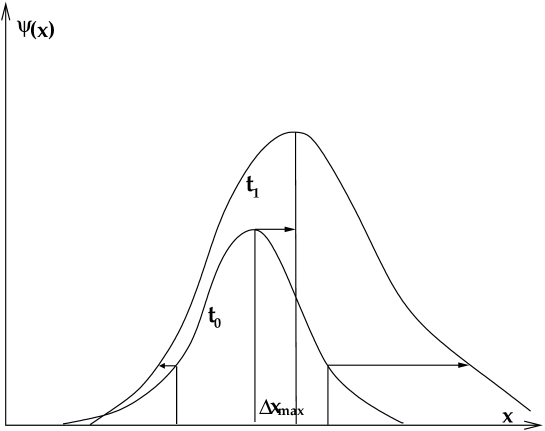
Figure 3: The propagation of an amplified signal $\psi(x,t)$. The location of the maximum describes the wave propagation

For a propagation of a kink front that experiences a deformation, one can check the translation of the second derivative of the shape, keeping track of the turning-point of the kink shape (Fig.4). In this case the second order (”three-point”) PV turns out to be the relevant velocity of propagation.

Figure 4: The propagation of a growing kink (”tsunami model”). The turning point is chosen to trace the propagation

Summarized, the local concept is based on local attributes of the wave shape being traced in course of propagation. The phase of an arbitrary wave in some point is characterized by the local Taylor expansion in this point. The local attribute of N-th order is therefore the N-th spatial derivative of the wave shape. The phase velocity of N-th order (N-PV) is the velocity of propagation of the corresponding N-th order attribute.

Finally, it should be noted, that the definiton of phase velocities of order zero and one, the $v_{(0)}$ and $v_{(I)}$ respectively, admits a straightforward generalization to two-, three-, and higher-dimensional propagation, while the phase velocities of second ( $v_{(II)}$) and higher orders inherently contain a certain element of ambiguity in their definition, since a possibility to choose a second-order attribute to be traced is not unique is not unique [19].

4 Examples

Let us consider the conventional 1+1-dimensional wave equation

$$\left[\frac{1}{a^{2}}\frac{\partial^{2}}{\partial t^{2}}-\frac{\partial^{2}}{\partial x^{2}}\right]\psi(x,t)=0$$ (4.1)

possessing translational solutions of the form

$$\psi(x,t)=\psi(t\pm\frac{x}{a}).$$ (4.2)

It is easy to check that in this case the PV’s of all orders defined above are identical and read

$$v_{(N)}(x,t)=a,\ \ \ \ N=0,1,2,...$$ (4.3)

which is nothing else but the classical phase velocity $\pm a$, thereby satisfying the a priori definition of ”phase velocity” itself as a medium constant in (4.1).

Let a propagating shape $\Psi$ now be subject to a temporal damping similar to (Fig.2) with

$$\Psi(x,t)=\psi(t-\frac{x}{a})e^{-\lambda t}\equiv\psi(\phi)e^{-\lambda t}$$ (4.4)

that obeys the wave equation (a typical field equation with a dynamical dissipation and a mass term)

$$\left\{\frac{1}{a^{2}}\frac{\partial^{2}}{\partial t^{2}}-\frac{\partial^{2}}{\partial x^{2}}+\frac{2\lambda}{a^{2}}\frac{\partial}{\partial t}+\frac{\lambda^{2}}{a^{2}}\right\}\Psi(x,t)=0$$ (4.5)

The ordinary 0-PV velocity reads

$$v_{(0)}=a\left(1-\lambda\frac{\psi}{\psi^{\prime}}\right),$$ (4.6)

where the prime denotes the derivative of $\psi$ with respect to its argument $\phi\equiv t-x/a$.

This result provides a velocity with bad physical features: the velocity grows for a descending shape, for an ascending shape it decreases, can even be negative, and it diverges exactly for the peak point (under the condition that the (measured) amplitude $\Psi$ as well as parameter $a,\lambda$ have positive values).

A relevant physical velocity in this case is for instance the 1-PV

$$v_{(I)}=a\left(1-\lambda\frac{\psi^{\prime}}{\psi^{\prime\prime}}\right)$$ (4.7)

providing for a peak being traced exactly the canonical phase velocity entering in the wave equation (4.5).

For this shape further PV’s of higher orders are given by (3.5):

$$v_{(N)}=a\left(1-\lambda\frac{\psi^{(n)}}{\psi^{(n+1)}}\right)\equiv a\left(1-\lambda(\log^{\prime}{\psi^{(n)}})^{-1}\right)$$ (4.8)

where $\psi^{(n)}$ denotes the $n$-th derivative of $\psi$ with respect to its argument as mentioned above. For an amplified signal as in Fig.3 we can e.g. change the sign of $\lambda$. Especially, for the case of a kink (Fig. 4)

$$\psi(t-\frac{x}{a})\equiv\psi(\phi)=\arctan\phi,$$ (4.9)

the spectrum of phase velocities reads by comparison :

$$v_{(0)}=a\left(1+\lambda(1+\phi^{2})\arctan\phi\right),$$

$$v_{(I)}=a\left(1-\lambda\frac{1+\phi^{2}}{2\phi}\right),$$ (4.10)

$$v_{(II)}=a\left(1-\lambda\frac{\phi^{3}+\phi}{3\phi^{2}-1}\right).$$

The ordinary 0-PV has an oscillating sign at $\lambda$ and is multiple defined because of the arctan function . Therefore it cannot be interpreted as a well-defined physical velocity. If the point being traced should be labelled by a derivative attribute, it turns out to be a physically inconvenient choice since the shape possesses no real peaks, whose propagation could be traced. Moreover the velocity $v_{(I)}$ diverges at $\phi=0$.

The possible labelled attribute is also the turning-point traced by the 2-PV. The velocity $v_{(II)}$ also possesses two singularities at $\phi=\pm 1/\sqrt{3}$ which do not coincide with the labelled point $\phi=0$, so it can be successfully followed up at the measurement.

Historical remark

The definition of a wave velocity proceeded with an extension of a translational solution of (4.1):

$$\psi(x,t)=\psi(t-\frac{x}{a})\equiv\psi[\frac{1}{\omega}(\omega t-\frac{\omega}{a}x)],\equiv\phi(\omega t-kx),\ k\equiv\frac{\omega}{a},$$ (4.11)

where the parameter $\omega$ has been interpreted as a frequency of a necessary perodic harmonic function $\phi$. usually $e^{\pm ix}$ as mentioned above in the introduction. It is not surprising that the 0-order PV provides in this case the value $\omega/k$, canonically interpreted as a phase velocity of periodic wave

In case of any interrelations between $k$ and $\omega$ that are not encountered in the wave equation, in particular any dispersion relation between frequency and wave-number, the PV $v_{(0)}$ is in fact a proportionality factor

$$d\omega=v_{(0)}dk,$$ (4.12)

which is identical with the classical definiton of a group velocity [1].

At this point it should be recalled, that the original idea of the group velocity $U$, as summarized e.g. in [28],

$$\frac{\partial\lambda}{\partial t}+U\frac{\partial\lambda}{\partial x}=0$$ (4.13)

was of the similar form as the recent definition (3.2) of 0-PV. It should be noted here that equation (4.13) involves local derivatives of the non-local parameter,i.e. the wavelength $\lambda$. For a variable wavelength much smaller than a vicinity of the point, this group velocity provides therefore a natural approximation to the zero-order phase velocity $v_{(0)}$.

In the present approach this feature appears as a physical phase velocity following in a straightforward way from the interpretation of phase propagation and does not require an interpretation of $\omega$ and $k$ as a frequency and wave number, as well as a constancy of some group respectively.

It is noted in passing, that in the case of a kink there are no suitable definitions of a wave group and of a concerned group velocity for this solution since a Fourier decomposition does not work on a non-compact support.

5 Lorentz covariance

The zero order PV (3.2 ) possesses an interesting property, i.e. a local covariance in the sense of special relativity, as shown now. This is not the case for PV’s of higher orders.

The PV $v_{(0)}$, measured in some stationary system $X$, takes in some other system $X^{\prime}$, moving with a constant speed $V$, via the Lorentz transformations

$$x^{\prime}=\frac{x-Vt}{\sqrt{1-\frac{V^{2}}{c^{2}}}},\ \ t^{\prime}=\frac{t-\frac{Vx}{c^{2}}}{\sqrt{1-\frac{V^{2}}{c^{2}}}}$$ (5.1)

the form

$$v^{\prime}_{(0)}=\frac{v_{(0)}+V}{1+\frac{v_{(0)}V}{c^{2}}}.$$ (5.2)

This means that the zero order PV respects the relativistic velocity addition. Especially, a subluminal zero order PV remains also subluminal in any other moving system $X^{\prime}$.

This result should not be a surprise, since the definition of the $v_{(0)}$ is implied by the condition:

$$\psi(x,t)=const,\ \$$ (5.3)

which remains to be of the same form under arbitrary transormations
$x=x(x^{\prime},t^{\prime});\ t=t(x^{\prime},t^{\prime})$, implying

$$d\psi(x,t)\equiv\frac{\partial\psi}{\partial t}dt+\frac{\partial\psi}{\partial x}dx=0$$ (5.4)

for the first order differential form (or simply first differential), which possesses a form-invariance property under transformations.

Since

$$v_{(0)}(x,t)=\frac{dx}{dt}$$ (5.5)

per definition, the equation (5.4) inplies the definition (3.2) of 0-PV, so it should behave under space-time transformations as a usual velocity of a matter point.

The first order PV (3.4), by comparison, evaluated in some system $X$ transformes in the moving system $X^{\prime}$ to:

$$v^{\prime}_{(I)}=-\frac{\left\{\left(1+\frac{V^{2}}{c^{2}}\right)\frac{\partial^{2}}{\partial x\partial t}-V\left(\frac{1}{c^{2}}\frac{\partial^{2}}{\partial t^{2}}+\frac{\partial^{2}}{\partial x^{2}}\right)\right\}\psi}{\left\{\frac{V^{2}}{c^{4}}\frac{\partial^{2}}{\partial t^{2}}+\frac{\partial^{2}}{\partial x^{2}}-2\frac{V}{c^{2}}\frac{\partial^{2}}{\partial t\partial x}\right\}\psi}.$$ (5.6)

If the pulse $\psi(x,t)$ obeys the free wave equation (4.1), the transformation becomes

$$v^{\prime}_{(I)}=-\frac{\left(1+\frac{V^{2}}{c^{2}}\right)v_{(I)}+2V}{\left(1+\frac{V^{2}}{c^{2}}\right)+\frac{2Vv_{(I)}}{c^{2}}},$$ (5.7)

i.e. a relation that should be called the ”first order velocity addition”. It differs obviously from the corresponding transformation of $v_{(0)}$, since the definition of the velocity $v_{(I)}$ results from the condition

$$d\left(\frac{\partial\psi(x,t)}{\partial x}\right)=0$$ (5.8)

whose form is explicitely non-invariant under space-time transformations.

It can be shown that a subluminal first order PV is still preserved by this transformation as well. Note, that for a signal which does not obey the free equation (4.1), this restriction is in general not guaranteed anymore.

6 A global velocity of signal transmission and ”dynamic separation”

The discussion of local velocities was aimed towards an evaluation of global features of signal propagation, namely the propagation through a finite spatial interval during a finite temporal interval. In other words, a global velocity, practically measured, means roughly the length of the distance $\Delta x$ traveled by a traced attribute divided by the time interval $\Delta t$.

The local PV’s of N-th order analyzed above can be interpreted as a first order differential equations of the form

$$v_{(N)}(x,t)=\frac{dx}{dt},$$ (6.1)

that can be illustrated graphically as a field of isoclines (Fig.5).

Figure 5: Phase velocities as a family of isoclines $v_{(N)}(x,t)$ and averaged global velocities between two events (measurements)

Here the local PV is the tangent function of the tangent vector of the isocline, and the averaged (total) velocity between $(t_{0},x_{0})$ and $(t_{1},x_{1})$ is represented by the tangent of the hypotenuse of the triangle $\{(t_{0},x_{0}),(t_{1},x_{1}),(t_{0},x_{1})\}$, (cf. Fig.5).

This procedure is elucidated best by some clear and well known examples. Consider the propagation of a translation mode of the form

$$\psi(x,t)=\psi(\xi t-k(x)):=\psi(\phi)$$ (6.2)

describing, for instance, an electromagnetic field propagation in an inhomogeneous dielectric medium. In this case, if the transversality of the wave not assured, the differential equation for any components of the field can possess e.g. a form like this:

$$\frac{n^{2}(x)}{c^{2}}\frac{\partial^{2}}{\partial t^{2}}\psi-\frac{\partial^{2}}{\partial x^{2}}\psi+\ln^{\prime}n(x)\frac{\partial}{\partial x}\psi=0$$ (6.3)

where $n(x)$ is the spatially dependent index of refraction. From the Ansatz (6.2) it results for the $k(x)$ from the optical inhomogeneity over the spatial coordinate $x$:

$$n(x)=\frac{c}{\xi}k^{\prime}(x),\ \ \ \ k(x)=\frac{\xi}{c}\int n(x)dx,$$ (6.4)

Then the local zero order PV is provided by eq.(3.2) and results in the first order equation

$$v_{(0)}(x,t)\equiv\frac{dx}{dt}=\frac{c}{n(x)},$$ (6.5)

that is a quite trivial result.

We proceed now with phase velocities of higher orders. For the 1-PV velocity $v_{(I)}$ defined by eq.(3.4) the same procedure leads to

$$v_{(I)}(x,t)\equiv\frac{dx}{dt}=\frac{c}{n(x)-\frac{c}{\xi}\frac{\psi^{\prime}}{\psi^{\prime\prime}}\ln^{\prime}n(x)}$$ (6.6)

where $x$ and $t$ denote the space and time location of the first oder attribute being traced; $\psi^{\prime}$and$\psi^{\prime\prime}$ are the first and the second derivative of the wave function $\psi$ with respect to its argument $\phi$ (cf.6.2). Similarly, for the 2-PV we obtain:

$$v_{(II)}(x,t)=\frac{dx}{dt}=\frac{c}{n(x)-3\frac{c}{\xi}\frac{\psi^{\prime\prime}}{\psi^{\prime\prime\prime}}\ln^{\prime}n(x)+\frac{c^{2}}{\xi^{2}}\frac{n^{\prime\prime}}{n^{2}}\frac{\psi^{\prime}}{\psi^{\prime\prime\prime}}}.$$ (6.7)

Suppose, we measured at the moment $t_{0}$ some value of the fisrt order attribute $\psi^{\prime}(x_{0})$ in the point $x_{0}$, and we are interested, where is this attribute to recover at the next moment $t_{1}$. For a maximum or a minimum point the result does not distinguish from the zero order velocity, as in the case considered above. Now, let we measured at $t_{0}$ some values:

$$\psi^{\prime}(0,x_{0}):=\psi_{0}^{\prime}\mbox{ and }\psi^{\prime\prime}(0,x_{0}):=\psi_{0}^{\prime\prime};\ \ \ \Lambda:=\psi^{\prime}(0,x_{0})/\psi_{0}^{\prime\prime}$$ (6.8)

An explicit integration of eq.(6.6) leads to

$$c(t_{1}-t_{0})=\int\limits_{x_{0}}^{x_{1}}n(x)dx-\Lambda\frac{c}{\xi}\ln\frac{n(x_{1})}{n(x_{0})}$$ (6.9)

for the interval of two events, where the signal attribute choosen for tracing has been checked at the time $t_{0}$ in the point $x_{0}$ and afterwards in $x_{1}$ at $t_{1}$. Let us assume that the point $(t_{0},x_{0})$ was not a critical point (i.e. of the knot type) of the equation (6.1). Then the global transition velocity between two points $x_{0},x_{1}$ is evaluated unique in such a way: divided by the spatial interval $x_{1}-x_{0}$ the eq.(6.9 ) provides the factor $\gamma$:

$$\gamma:=c\frac{t_{1}-t_{0}}{x_{1}-x_{0}}=\frac{1}{x_{1}-x_{0}}\left[\int\limits_{x_{0}}^{x_{1}}n(x)dx-\Lambda\frac{c}{\xi}\ln\frac{n(x_{1})}{n(x_{0})}\right]$$ (6.10)

It follows, that a value of $\gamma$ less than 1 is not prohibited in principle even for real $n>1$, that means a superluminal averaged global velocity along the finite distance. A similar result appears for 2-PV and higher orders. A numerical examples for dielectric media of special modulation confirms this possibility [27]. The discussion of physical interpretation of this result is still open.

It is also worth to notice, that for the first order PV (as well as the second and higher orders) in media with a variable refraction index $n(x)$ an essential dependence on the parameter $\xi$ enters.

The meaning of $\xi$ can be derived from the given form of the solution $\psi$. It can be interpreted, for instance, as a frequency factor for a periodic mode or a damping factor for an evanescent mode. This parameter simply means an enumeration of solutions of a solution family (space of solutions). The merit gained above is the separation of these solutions with respect to the parameter $\xi$ by the different first (and higher)-order PV’s through the inhomogeneity of the medium.

In the case of a periodic wave for instance, it can be interpreted as a dispersion although an explicit frequency-dependence of $n(x)$ was not assumed. Moreover, the parameter $\xi$ has not necessarily to be interpreted as a frequency of some temporally periodic oscillation, but rather as a time component of the space-time wave vector $\{\omega,{\bf k}\}$ for a translation mode (4.2) in a general form. The phenomenon considered thus has another origin and is much more general as a conventional non-localized frequency dispersion $n(\omega)$

Thus we established for the first (and higher) order PV’s in optical inhomogeneous media the essential dependence on the t-component $\omega$ of the wave translation vector, especially frequency, even for local non dispersive media, which could be called ”dynamic separation”. The global averaged dynamic separation of eq. (6.9) survives as a corollary of the local separation of (6.6). This phenomena does not occur for the ordinary zero order PV.

7 Concluding remarks

The inherent inconsistency of the classical subjects of phase velocity and group velocity, (as well as signal velocity based therein) has been discussed. The inapplicability of these concepts for actual studies in photonics, near-field and nano-optics has been shown to result from the essential non-locality of these definitions.

An alternative approach for description of a propagation velocity has been proposed. It is strictly local and is based on the natural assumption of an ordinary measurement procedure. It does not need any a priori condition of periodicity, frequency, groups and packets or other canonical attributes.

The definitions presented above are applicable in a natural way for arbitrary waves and pulses. In a mathematical sense they describe a propagation of a perturbation in any field in space-time. Examples could be: an acoustic wave as a pressure perturbation, a gravitation wave on a fluid surface, a spin wave in a solid state a.s.f. In particular, the formalism is very suited for the description of particle propagation in field theory, where particles are considered as field perturbations.

This approach results in the set of measurable propagation velocities. In zeroth order the propagation velocity coincides with the ordinary phase velocity and appears to be ordinary Lorentz covariant; further application gives rise to generate ”Lorentz covariance of higher orders”.

For propagation in inhomogeneous media, for instance for light in a medium with a space-dependent index of refraction, phase velocities of higher orders show some remarkable properties:

a) they are not restricted in general by the speed of light in vacuum;

b) they exhibit an essential dependence on the time component of the wave vector solely as a result of inhomogeneity, treated canonically as a ”dispersion”. This appears to be a more general phenomena, and does not presuppose any periodic frequency and dispersive properties of media. It should be called for this reason ”dynamic separation” [27].

Further applications, like photonics and optoelectronics are dealing with signals i.e. non-localized objects, represented as a cut of wave shape between labelled points possessing a certain spatial length (or temporal duration). These two points are marked by a value of zeroth order attribute (e.g. a voltage amplitude), or by a first order one (a block between an ascent and a descent of amplitude). In this sense the signal is considered as not a local, but at least a bi-local object. Its propagation can be traced by an averaged bilocal velocity, constructed from local ones in a natural way.

The same concerns a propagation of single photons, especially of low energy, which are non-localized objects. For the case of evanescent modes we are dealing yet with a sufficient delocalization.

Another approach to the signal transmission is based on a pure local signals, which can be, for instance, a point of discontinuity, propagating away from the perturbation [18]. For these problems the velocities of higher orders, especially 1-PV and 2-PV provide a suitable tool, as shown above. In this context are the velocities 1-PV and 2-PV of special interest, being treated in pure physical sense as a true speed of interaction.

References

- [1] L. Brillouin Wave Propagation and Group Velocity NEW YORK (U. A.): ACADEMIC PR., 1960. - XI,154 S. , 1960 .
- [2] M. Born, E. Wolf Principles of Optics, Cambridge University Press, 1999
- [3] G. C. Sherman, K. E. Oughstun, Phys.Rev.Lett., 47 (20), 1451-1454 (1981)
- [4] K. E. Oughstun, N. A. Cartwright J.Mod.Opt., 52 (8), 1089-1104 (2005)
- [5] M. Centini, M. Bloemer, K. Myneni, M. Scalora, C. Sibilia, M. Bertolotti, G. D’Aguanno, Phys.Rev.E, 68 016602 (2003)
- [6] G. Nimtz and W. Heitman, Prog.Quant.Electronics 21, (1997)
- [7] A. Gürtler, C. Winnewisser, H. Helm, P. U. Jepsen J.Opt.Soc.Am.A, 17 (1), 74-83 (2000)
- [8] T. Kohmoto, H. Tanaka, S. Furue, K. Nakayama, M. Kunimoto, Y. Fukuda, Phys.Rev. A, 72, 025802 (2005)
- [9] A. Bers, Am.J.Phys., 68(5), 482-484 (2000)
- [10] N. S. Shiren, Phys.Rev.A, 128 (5), 2103-2112 (1962)
- [11] R. Loudon, J.Phys.A , 3 233-245(1970)
-
[12]
T. Kohmoto, S. Furue, Y. Fukui, K. Nakayama, M. Kunimoto, Y. Fukuda,
Technical Digest. Summaries of papers presented at the Quantum Electronics and Laser Science Conference.
Conference Edition (IEEE Cat. No.02CH37338) (2002) Vol.1 p.241 Vol.1 of (271+40 suppl.)pp., - [13] S. C. Bloch, Am.J.Phys., 45 (6), 538-549 (1976)
- [14] H. M. Nussenzveig, Causality and dispersion relations New York Acad. Press 1972
- [15] E. Sonnenschein, I. Rutkevich, D. Censor, J.Electromagneic Waves and Appl., 14 (4), 563-565 (2000)
- [16] H. P. Schriemer, J. Wheeldon, T. Hall Proc.SPIE, Int.Soc.Opt.Eng.2005, 5971, 597104.1-597104.9 (2005)
- [17] A. Gomez, A. Vegas, M. A. Solano Microwave and Opt.Technol.Lett., 44 (3), 302-303 (2005)
- [18] M. D. Stenner et al., Phys.Rev.Lett.94 053902 (2005); M. D. Stenner et al., Nature 425, (2003)625
- [19] I. Drozdov, A. Stahlhofen, arXiv: math-ph/0701022, to be published
- [20] D. K. Hoffmann, M. Arnold, D. J. Kouri J.Phys.Chem.(1993), 97(6) ,1110-18
- [21] K. Aric, R. Gutdeutsch, A. Sailer J.Pure and Applied Geophys.(1980), 118(3), 796-806
- [22] Z. Xiaoming, J. M Greenleaf Ultrasound in Med.and Biol. (Nov.2006) 32(11) 1655-60
- [23] J. A. Simmons J.Acoust.Soc.Am. (1992) 92(2) 1061-90
- [24] A. Gonzalez-Serrano, J. F. Claerbout Geophysics(Sept 1984) 49(9) 1432-56
- [25] S. Al Rabadi, L. Friedel, A. Al Salaymeh Chem.Eng.Tec.(2007) 30(1) 71-83
- [26] C. Pacher, W. Boxleitner, E. Gornik Phys.Rew.B, 71 (12), 125317-1-11 (2005)
- [27] I. Drozdov, A. Stahlhofen, in preparation
- [28] H. Bateman, Partial Differential Equations of Mathematical Physics Cambridge University Press, 1969 (orig.1931) p.231