Possible experimental manifestations of the many-body localization

Abstract

Recently, it was predicted that if all one-electron states in a non-interacting disordered system are localized, the interaction between electrons in the absence of coupling to phonons leads to a finite-temperature metal-insulator transition. Here, we show that even in the presence of a weak coupling to phonons the transition manifests itself (i) in the nonlinear conduction, leading to a bistable $I$-$V$ curve, (ii) by a dramatic enhancement of the nonequilibrium current noise near the transition.

Introduction.— Low-temperature charge transport in disordered conductors is governed by the interplay between elastic scattering of electrons off static disorder (impurities) and inelastic scattering (electron-electron, electron-phonon, etc.). At low dimensions an arbitrarily weak disorder localizes Anderson58 all single-electron states Gertsenshtein ; Abrahams , and there would be no transport without inelastic processes. For the electron-phonon scattering, the dc conductivity $\sigma(T)$ at low temperatures $T$ is known since long ago Mott : in $d$ dimensions

$$\ln\sigma(T)\propto-1/T^{\gamma},\quad\gamma=1/(d+1)\,.$$ (1)

What happens if the only possible inelastic process is electron-electron scattering? The answer to this question was found only recently us : $\sigma(T)=0$ identically for $T<T_{c}$, the temperature of a metal-insulator transition. Here we discuss experimental manifestations of this transition in real systems, where both electron-electron and electron-phonon interactions are present. We show that (i) the $I$-$V$ characteristic exhibits a bistable region, and (ii) non-equilibrium current noise is enhanced near $T_{c}$.

The notion of localization was originally introduced for a single quantum particle in a random potential Anderson58 . Subsequently, the concept of Anderson localization was shown to manifest itself in a broad variety of phenomena in quantum physics. This concept can also be extended to many-particle systems. Statistical physics of many-body systems is based on the microcanonical distribution, i. e., all states with a given energy are assumed to be realized with equal probabilities. This assumption means delocalization in the space of possible states of the system. It does not hold for non-interacting particles; however, it is commonly believed that an arbitrarily weak interaction between the particles eventually equilibrates the system and establishes the microcanonical distribution.

Many-body dynamics of interacting systems and its relation to Anderson localization has been discussed in the context of nuclear Agassi and molecular Wolynes physics. For interacting electrons in a chaotic quantum dot this issue was raised in Ref. AGKL , where it was shown that electron-electron interaction may not be able to equilibrate the system. This corresponds to Anderson localization in the many-body space. Recently it was demonstrated that in an infinite low-dimensional system of (weakly) interacting electrons, subject to a static disorder, Anderson transition in the many-body space manifests itself as a finite-temperature metal-insulator transition us .

Figure 1: Schematic temperature dependence of the dc conductivity $\sigma(T)$ for electrons subject to a disorder potential localizing all single particle eigenstates, in the presence of weak short-range electron-electron $\lambda\delta_{\zeta}$, $\lambda\ll{1}$, established in Ref. us . Below the point of the many-body metal-insulator transition, $T<T_{c}\sim\delta_{\zeta}/|\lambda\ln\lambda|$, no inelastic relaxation occurs and $\sigma(T)=0$. At $T\gg\delta_{\zeta}/\lambda^{2}$ the high-temperature metallic perturbation theoryAA is valid, and corrections to the Drude conductivity $\sigma_{\infty}$ are small. In the interval $\delta_{\zeta}/\lambda\ll{T}\ll\delta_{\zeta}/\lambda^{2}$ electron-electron interaction leads to electron transitions between localized states, and the conductivity depends on temperature as a power-law.

Let single-particle eigenstates be localized on a spatial scale $\zeta_{loc}$ (localization length). The characteristic energy scale of the problem is the level spacing within the localization volume: $\delta_{\zeta}=1/(\nu\zeta_{loc}^{d})$, $\nu$ being the density of states per unit volume. Below we neglect energy dependences of $\nu$, $\zeta_{loc}$, and $\delta_{\zeta}$. According to Ref. us , as long as electrons are not coupled to any external bath (such as phonons), a weak short-range electron-electron interaction (of typical magnitude $\lambda\delta_{\zeta}$, with the dimensionless coupling constant $\lambda\lesssim{1}$) does not cause inelastic relaxation unless the temperature $T$ exceeds a critical value:

$$T_{c}\sim\frac{\delta_{\zeta}}{|\lambda\ln\lambda|}.$$ (2)

The small denominator $|\lambda\ln\lambda|$ represents the characteristic matrix element of the creation of an electron-hole pair. The ratio $T_{c}/\delta_{\zeta}$ is the number of states available for such a pair (in other words, the phase volume) at $T=T_{c}$. Only provided that this number is large enough to compensate the smallness of the matrix element, the interaction delocalizes the many-body states and thus leads to an irreversible dynamics. As a result, the finite-temperature dc conductivity $\sigma(T)$ vanishes identically if $T<T_{c}$, while $\sigma(T>T_{c})$ is finite, i. e. at $T=T_{c}$ a metal-insulator transition occurs. The overall dependence $\sigma(T)$ is summarized in Fig. 1.

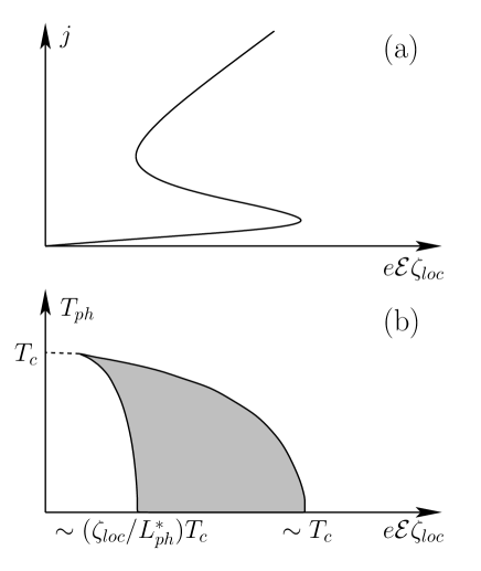
Figure 3: (a) sketch of the bistable $I$-$V$ curve for a fixed value of $T_{ph}$; (b) $(\mathcal{E},T_{\rm ph})$-plane with the bistable region schematically shown by shading. The dashed line represents the crossover between the metallic state at high electric field $\mathcal{E}$ or high phonon temperature $T_{ph}$, and the insulating state at low $\mathcal{E}$ and low $T_{ph}$.

In any real system the electron-phonon interaction is always finite. This makes $\sigma(T)$ finite even at $T<T_{c}$: $\sigma(T)$ is either exponentially small [Eq. (1)] at $T\ll\delta_{\zeta}$, or follows a power-law GMR at $\delta_{\zeta}\ll{T}\ll{T}_{c}$. At the transition point the phonon-induced conductivity is not exponentially small, i. e. phonons smear the transition into a crossover. Are there any experimental signatures of the many-body localization? In what follows we show that if the electron-phonon coupling is weak enough, a qualitative signature of the metal-insulator transition can be identified in the nonlinear conduction. Namely, in a certain interval of applied electric fields $\mathcal{E}$ and phonon temperatures $T_{ph}$ both metallic and insulating states of the system turn out to be stable! As a result, the $I$-$V$ curve exhibits an S-shaped bistable region (Fig. 3). Moreover, we show that the many-body character of the electron conduction dramatically modifies the non-equilibrium noise near the transition [Eq. (12)].

Bistable $I$-$V$ curve.— Our arguments are based on two observations. First, in the absence of phonons a weak but finite electric field cannot destroy the insulating state – it rather shifts the transition temperature. Let us neglect the effect of the field on the single-particle wave functions, representing it as a tilt of the local chemical potential of electrons. Then at $T=0$ the role of the field in the insulating regime is increase the energy of the electron-hole (e-h) excitation of a size $L$ by $e\mathcal{E}L$. This provides in additional phase volume of the order of $e\mathcal{E}L/\delta_{\zeta}$. However, for $L>\zeta_{loc}$ the matrix element for creation of such an excitation quickly vanishes. In the diagrammatic language for the effective model of Ref. us this means that each electron-electron interaction vertex must be accompanied by tunneling vertices which describe coupling between localization volumes and whose number is (i) at least one in order to gain phase volume (in contrast to the finite-$T$ case when tunneling had to be included only to overcome the finiteness of the phase space in a single grain us ), and (ii) not much greater than one, otherwise the diagram is exponentially small. As a result, at $T=0$ the insulator state is stable provided that $\mathcal{E}<\mathcal{E}_{c}\sim{T}_{c}/(e\zeta_{loc})$.

In the same way one can analyze the finite-temperature correction to the critical field, and the finite-field correction to the critical temperature can be found by taking into account the extra phase volume in the calculation of Ref. us . One obtains $\sigma(T)=0$ for $T<T_{c}(\mathcal{E})$, where

$$T_{c}(\mathcal{E})=T_{c}-c_{1}{e}\mathcal{E}\zeta_{loc}\,.$$ (3)

with a model-dependent factor $c_{1}\sim{1}$, weakly dependent on $\mathcal{E}$ [here and below $T_{c}$ without the argument $\mathcal{E}$ is the zero-field value given by Eq. (2)]. As a consequence, at $T<{T}_{c}(\mathcal{E})$ the nonlinear transport, as well as the linear one, has to be phonon-assisted.

The second observation is that when both $\sigma$ and $\mathcal{E}$ are finite, there is Joule heating. The thermal balance is qualitatively different in the insulating and the metallic phases. Deep in the insulating phase ($T\ll{T}_{c}$) each electron transition is accompanied by a phonon emission/absorption, i. e. electrons are always in equilibrium with phonons whose temperature $T_{ph}\ll{T}_{c}$ we assume to be fixed. On the contrary, in the metallic phase electrons gain energy when drifting in the electric field, i. e. they are heated. Due to this Joule heating the effective electron temperature $T_{el}$ deviates from the bath temperature. The role of phonons is then to stabilize $T_{el}$. For weak electron-phonon coupling $T_{el}$ and $T_{ph}$ can differ significantly. A self-consistent estimate for $T_{el}$ follows from

$$T_{el}-T_{ph}\sim{e}\mathcal{E}L_{ph}(T_{el})\,,$$ (4)

$$L_{ph}(T_{el})=\sqrt{D(T_{el})\,\tau_{ph}(T_{el})}\,.$$ (5)

Here $\tau_{ph}(T_{el})$ is the time it takes an electron to emit or absorb a phonon, $L_{ph}(T_{el})$ is the typical electron displacement during this time, and $D(T_{el})=\sigma(T_{el})/(e^{2}\nu)$ is the electron diffusion coefficient.

Figure 2: Sketch of the dependences $(T_{el}-T_{ph})/({e}\mathcal{E})$ (dashed line) and $L_{ph}(T_{el})$ (solid lines, electron-phonon coupling strength being weaker for higher curves). Actual value of $T_{el}$ is determined by their crossing.

We sketch in Fig. 2 $(T_{el}-T_{ph})/({e}\mathcal{E})$ and $L_{ph}(T_{el})$ for different electron-phonon coupling strengths as functions of $T_{el}$. It is taken into account that (i) $L_{ph}$ coincides with variable range hopping length at $T_{el}\ll\delta_{\zeta}$, (ii) $L_{ph}\sim\zeta_{loc}$ at $\delta_{\zeta}\ll{T}_{el}\ll{T}_{c}(\mathcal{E})$, (iii) $D(T_{el})$ quickly rises to its large metallic value $D_{\infty}\sim\delta_{\zeta}\zeta_{loc}^{2}$ near $T_{c}(\mathcal{E})$, (iv) $\tau_{ph}(T_{el})$ decreases as a power law with increasing $T_{el}$. The peak of the curve rises with decreasing electron-phonon coupling strength, and eventually the curve crosses the straight line. After that, in addition to $T_{el}=T_{ph}$, Eq. (4) acquires two more solutions, both with $T_{el}>T_{c}(\mathcal{E})$, of which only the rightmost solution is stable. The maximum of $L_{ph}$ can be estimated as $L_{ph}^{*}\sim\sqrt{D_{\infty}\tau_{ph}(T_{c})}$, so three solutions appear when ${T}_{c}(\mathcal{E})-T_{ph}\ll{e}\mathcal{E}L_{ph}^{*}$. At the same time, as seen from Eq. (3), electric field is unable to break down the insulator as long as ${e}\mathcal{E}\zeta_{loc}\ll{T}_{c}-T_{ph}$. Thus, the interval of electric fields where both regimes are stable, is determined by

$$\frac{{T}_{c}(\mathcal{E})-T_{ph}}{eL_{ph}^{*}}\ll\mathcal{E}\ll\frac{{T}_{c}-T_{ph}}{e\zeta_{loc}}\,.$$ (6)

The two conditions are compatible provided that

$$L_{ph}^{*}\gg\zeta_{loc}\,,$$ (7)

which is realistic when electron-phonon coupling is weak.

In the bistable region (6), for a given value of $\mathcal{E}$ one finds two stable solutions for $T_{el}$, giving two possible values of the conductivity and the current, which corresponds to an $S$-shape current-voltage characteristic Scholl , the third (unstable) solution corresponding to the negative differential conductivity branch. The macroscopic consequences of such behavior depend on the dimensionality. In a 2d sample the two phases of different electronic temperature and current density can coexist, separated by a boundary of the width $\sim{L}_{ph}^{*}$, parallel to the direction of the electric field. The particular state of the system determined by the boundary conditions (properties of the external circuit), as well as by the history.

Noise enhancement.— In the vicinity of the critical point conduction is dominated by correlated many-electron transitions (electronic cascades). Each cascade is triggered by a single phonon. As $T_{el}\to{T}_{c}(\mathcal{E})$, the typical value $\bar{n}$ of the number $n$ of electrons in the cascade diverges together with the time duration of a cascade. The results of Ref. us , adapted for a finite electric field, give the following probability for an $n$-electron transition to go with the rate $\Gamma$:

$$P_{n}(\Gamma)=\sqrt{\frac{\bar{\Gamma}_{n}}{4\pi}}\frac{e^{-\bar{\Gamma}_{n}/(4\Gamma)}}{\Gamma^{3/2}}\,,\quad\bar{\Gamma}_{n}\propto\left(\frac{T_{el}+c_{1}e\mathcal{E}\zeta_{loc}}{T_{c}}\right)^{2n},$$ (8)

which gives

$$1/\bar{n}\sim\ln[T_{c}/(T_{el}+c_{1}e\mathcal{E}\zeta_{loc})].$$ (9)

The divergence in $\bar{n}$ is cut off when electron-phonon coupling is finite. The largest $\bar{n}$ is such that the phonon broadening of the single-electron levels, $1/\tau_{ph}(T_{c})$, is comparable to $\bar{n}$-particle level spacing (in other words, time duration of a cascade cannot exceed $\tau_{ph}$):

$$\frac{1}{\tau_{ph}(T_{c})}\sim\delta_{\zeta}\left(\frac{\delta_{\zeta}/\bar{n}^{\alpha{d}}}{{T}_{c}}\right)^{4\bar{n}}\;\;\;\Rightarrow\;\;\;\bar{n}_{max}\sim\frac{1}{4}\frac{\ln(\delta_{\zeta}\tau_{ph})}{\ln(T_{c}/\delta_{\zeta})}\,,$$ (10)

with logarithmic precision; $\bar{n}^{\alpha}$ represents the divergent spatial extent of the cascade (correlation length) index .

Each many-electron transition can be characterized, besides its rate $\Gamma$, by the total dipole moment $\vec{d}$ it produces. The corresponding backward transition produces the dipole moment $-\vec{d}$ and goes with the rate $\Gamma{e}^{-(\vec{\mathcal{E}}\cdot\vec{d})/T_{el}}$ localfield . The average current $\langle{I}(t)\rangle$ is determined by the difference between forward and backward rates; obviously, it vanishes for $\mathcal{E}=0$. At the same time, the noise power (second cumulant) $S_{2}\equiv\int[\langle{I(t)I(t^{\prime})}\rangle-\langle{I(t)}\rangle\langle{I(t^{\prime})}\rangle]\,dt^{\prime}$ is determined by the sum of the forward and backward rates; at $\mathcal{E}=0$ it is given by the equilibrium Nyquist-Johnson expression.

Equilibrium noise carries no information about the nature of conduction. To see a signature of many-electron transitions it would be natural to analyze the shot noise, whose power is proportional to the charge transferred in a single event. Many-electron cascades would then correspond to “bunching” of electrons, thus increasing the shot noise. However, shot noise is observed in the limit when transitions transferring charge only in one direction (namely, $\vec{d}\cdot\vec{\mathcal{E}}>0$) are allowed, i. e. $T_{el}\ll{e}\mathcal{E}\zeta_{loc}$, which is impossible to satisfy in the insulating state, as $T_{el}\sim\max\{T_{ph},e\mathcal{E}\zeta_{loc}\}$ Levin . Thus, $S_{2}$ inevitably has both equilibrium and non-equilibrium contributions, which are difficult to separate.

To see the “bunching” effect unmasked by a large thermal noise at low fields one should study the third Fano factor $S_{3}$ of the current fluctuations Levitov . Indeed, being proportional to an odd power of the current, it vanishes in equilibrium, so it is not subject to the problems described above for $S_{2}$. In a wire of length $L$ the ratio $S_{3}/\langle{I}\rangle$ is given by

$$\frac{S_{3}}{\langle{I}\rangle}=\frac{L^{-3}\left\langle\!\left\langle\Gamma{d}^{3}\right\rangle\!\right\rangle}{L^{-1}\left\langle\!\left\langle\Gamma{d}\right\rangle\!\right\rangle}\,.$$ (11)

The double angular brackets on the right-hand side mean the sum over all allowed transitions. For nearest-neighbor single-electron transitions with $d=\pm{e}\zeta_{loc}$ Eq. (11) gives $S_{3}/\langle{I}\rangle\sim{e}^{2}(\zeta_{loc}/L)^{2}$, which is analogous to the Schottky expression reduced by the effective number of tunnel junctions in series, $L/\zeta_{loc}$, for $S_{2}$ Landauer .

Since $d^{3}$ diverges stronger than $d$ as $\bar{n}\to\infty$, we expect a divergence in Eq. (11). The critical index of $d$ depends on the order of limits: $d\sim\sqrt{n}{e}\zeta_{loc}$ if the linear response limit $\mathcal{E}\to{0}$ is taken prior to $\bar{n}\to\infty$, while $d\sim{n}{e}\zeta_{loc}(e\mathcal{E}\zeta_{loc}/T_{c})$ for a small but finite $\mathcal{E}$. As a result,

$$\frac{S_{3}}{\langle{I}\rangle}\sim\left(\frac{e\zeta_{loc}}{L}\right)^{2}\max\left\{\bar{n}\,,\left(\frac{\bar{n}e\mathcal{E}\zeta_{loc}}{T_{c}}\right)^{2}\right\},\quad\bar{n}\lesssim\bar{n}_{max}\,,$$ (12)

where $\bar{n}$ is given by Eq. (9), and the saturation of the divergence is determined by Eq. (10). Upon further increase of the temperature, the system crosses over to the metallic state, and $\bar{n}$ starts to decrease. This decrease is governed by the same Eq. (10) with the phonon inelastic rate substituted by the typical value of the electron-electron inelastic rate, which grows with temperature. As the critical behavior of $\Gamma$ on the metallic side of the transition is unknown, we cannot give any quantitative estimate of $S_{3}$ above $T_{c}$.

Conclusions.— In conclusion, we have shown that the finite-temperature metal-insulator transition, predicted theoretically in Ref. us , can manifest itself on the macroscopic level as an S-shape current-voltage characteristic with a bistable region. In fact, the hysteretic behaviour of the current in Y_xSi_1-x Ladieu is a possible candidate for the effect discussed in the present paper.

Besides, we have shown that the many-body nature of the conduction near the transition manifests itself in the dramatic increase of the non-equilibrium current noise: the noise depends on the total charge transferred in each random event, while the number of electrons, involved in such an event, increases as one approaches the transition.

We acknowledge discussions with M. E. Gershenson, C. M. Marcus, A. K. Savchenko, M. Sanquer, and thank H. Bouchiat for drawing our attention to Ref. Ladieu .

References

- (1) P. W. Anderson, Phys. Rev. 109, 1492 (1958).
- (2) M. E. Gertsenshtein and V. B. Vasil’ev, Teoriya Veroyatnostei i ee Primeneniya 4, 424 (1958) [Theory of Probability and its Applications 4, 391 (1958)].
- (3) E. Abrahams, P. W. Anderson, D. C. Licciardello, and T. V. Ramakrishnan, Phys. Rev. Lett. 42, 673 (1979).
- (4) N. F. Mott, J. Non-Cryst. Solids 1, 1 (1968); Mott formula does not into account Coulomb interaction, which changes the value of in Eq. (1) [A. L. Efros and B. I. Shklovskii, J. Phys. C 8, L49 (1975)].
- (5) D. M. Basko, I. L. Aleiner, and B. L. Altshuler, Ann. Phys. 321, 1126 (2006). See also cond-mat/0602510.
- (6) D. Agassi, H. A. Weidenmüller, and G. Mantzouranis, Phys. Rep. 22, 145 (1975).
- (7) D. E. Logan and P. G. Wolynes, J. Chem. Phys. 93, 4994 (1990).
- (8) B. L. Altshuler, Y. Gefen, A. Kamenev, and L. S. Levitov, Phys. Rev. Lett. 78, 2803 (1997).
- (9) B. L. Alshuler and A. G. Aronov, in Electron-Electron Interactions in Disordered Systems, ed. by A. L. Efros and M. Pollak (Elsevier, Amsterdam, 1985).
- (10) A. A. Gogolin, V. I. Melnikov, and É. I. Rashba, Zh. Eksp. Teor. Fiz. 69, 327 (1975) [Sov. Phys. JETP 42, 168 (1976)].
- (11) E. Schöll, Nonlinear Spatio-Temporal Dynamics and Chaos in Semiconductors (Cambridge University Press, Cambridge, 2001).
- (12) The index depends on the dimensionality only. Arguments given in Sec. 6.5 of Ref. us fix in 1d, and restrict in 2d, in 3d, in higher dimensions.
- (13) Strictly speaking, the electric field appearing in Eq. (8) is the local electric field, resulting from the spatial redistribution of charge over the random resistor network. Here we neglect fluctuations of the local field (more precisely, their correlations with the spatial fluctuations in and ), and understand as the external field. This is a good approximation for the distribution (8), as the current pattern is determined by the typical resitors, .
- (14) B. I. Shklovskii, Fiz. Tekh. Poluprovodn. 6, 2335 (1972) [Sov. Phys. Semicond. 6, 1964 (1973)]; B. I. Shklovskii, E. I. Levin, H. Fritzsche, and S. D. Baranovskii, in Transport, Correlation and Structural Defects, edited by H. Fritzsche (World Scientific, Singapore, 1990).
- (15) L. S. Levitov and M. Reznikov, cond-mat/0111057; Phys. Rev. B 70, 115305 (2004).
- (16) R. Landauer, Physica B 227, 156 (1996); A. N. Korotkov and K. K. Likharev, Phys. Rev. B 61, 15975 (2000).
- (17) F. Ladieu, M. Sanquer, and J. P. Bouchaud, Phys. Rev. B 53, 973 (1996).