, and

Trajectory of neutron$-$neutron$-^{18}C$ excited three-body state

Abstract

The trajectory of the first excited Efimov state is investigated by using a renormalized zero-range three-body model for a system with two bound and one virtual two-body subsystems. The approach is applied to $n-n-^{18}$C, where the $n-n$ virtual energy and the three-body ground state are kept fixed. It is shown that such three-body excited state goes from a bound to a virtual state when the $n-^{18}$C binding energy is increased. Results obtained for the $n-^{19}$C elastic cross-section at low energies also show dominance of an $S-$matrix pole corresponding to a bound or virtual Efimov state. It is also presented a brief discussion of these findings in the context of ultracold atom physics with tunable scattering lengths.

PACS 03.65.Ge, 21.45.+v, 11.80.Jy, 21.10.Dr

The interest on three-body phenomena occurring for large two-body scattering lengths have increased in the last years in view of the experimental possibilities presented in ultracold atomic systems, where the two-body interaction can be tunned by using Feshbach resonance techniques. Theoretical predictions, well investigated for three particle systems, such as the increasing number of three-body bound states when the two-body scattering length goes to infinity - known as Efimov effect [1] - can actually be checked experimentally in ultracold atomic laboratories. Indeed, the first indirect evidence of Efimov states came from recent experiments with ultracold trapped Caesium atoms made by the Innsbruck group [2].

In the nuclear context, the investigations of Efimov states are being of renewed interest with the studies on the properties of exotic nuclei systems with two halo neutrons ($n-n$) and a core ($c$). One of the most promising candidates to present these states is the ²⁰C [3, 4, 5] ($c\equiv^{18}C$). ²⁰C has a ground state energy of 3.5 MeV with a sizable error in $n-^{18}$C two-body energy, 160$\pm$110 keV [6].

The proximity of an Efimov state (bound or virtual) to the neutron-core elastic scattering cut makes the cross-section extremely sensitive to the corresponding $S$-matrix pole. However, one should be aware that the analytic properties of the $S$-matrix for Borromean systems (where all the two-body subsystems are unbound, like the Caesium atoms of the Innsbruck experiment [2]) are expected to be quite different from systems where at least one of the two-body subsystems are bound, as the present case of $n-n-^{18}$C.

The trajectory of Efimov states for three particles with equal masses has been studied in [7, 8] using the Amado model [9]. By studying the $S-$matrix in the complex plane, varying the two-body binding, it was confirmed previous analysis [8, 10], that Efimov bound states disappear into the unphysical energy sheet associated to the unitarity cut, becoming virtual states. It was also verified that, by further increasing the two-body binding, the corresponding pole trajectories remain in the imaginary axis and never become resonant.

Considering general halo-nuclei systems ($n-n-c$), in [3] it was mapped a parametric region defined by the $s-$wave two-body (bound or virtual) energies, where the Efimov bound states can exist. By increasing the binding energy of a two-body subsystem, it was noted that the three-body bound state turns out to a virtual state, remaining as virtual with further increasing of the two-body binding, as already verified in [8, 11]. In the other side, starting with zero two-body binding, by increasing the two-body virtual energy we have the three-body energy going from a bound to a resonant state [12].

Actually, the analysis of the trajectory of Efimov states in the complex plane can be relevant to study properties of the ²⁰C. In order to study the behavior of Efimov states, the authors of [4] have recently pointed out the importance of the analysis of low energy $n-^{19}$C elastic scattering observables. Their results, leading to a ²⁰C resonance prediction near the scattering threshold [4], when the separation energy of the bound halo neutron of ¹⁹C is changed, suggest a different behavior from the one found for three equal-mass particles, where a bound Efimov state turns into a virtual one as the two-body binding increases. In view of the importance of the results, not only in the nuclear context, it is interesting to consider a new independent analysis of three-particle systems where two subsystems are bound and one is unbound, considering particularly the case with different masses. As we show in the present letter, the results of our treatment for three-body system with unequal masses are consistent with the expectation derived from equal mass systems. Moreover, they are model independent due to the universal character of the three-body physics at very low energies. See Ref. [13] for a comment on the results obtained in Ref. [4].

In order to clarify the behavior (in the complex energy plane) of a given Efimov state for the $n-n-^{18}$C system, we consider the $n-c$ subsystem bound with varying energies; the virtual energy of the $n-n$ subsystem and the ground state energy of ²⁰C are fixed, respectively, at $-$143 keV [14, 15] and $-$3.5 keV (these constraints are convenient to follow the trajetory of the excited Efimov states since their appearance/disappearance depends only on the ratio of the $n-c$ and $n-n-c$ energies, see pages 327-329 of Ref. [16]). Our present study of $n-n-^{18}$C can be easily extended to similar systems such as ¹²Be, ¹⁵B, ²³N and ²⁷F.

In the present case, the bound state equations are extended to the second Riemann energy sheet through the $n-^{19}$C elastic scattering cut (see Fig. 1) using a well-known technique [17]. Consistent with previous results [3, 8, 11] for three equal masses particles, by using the present approach that will be explained in the following, we conclude that (also in this case) the three-body bound state turns into a virtual (and not a resonance) one when we increase the $n-^{18}$C two-body binding energy. The full behavior of the Efimov virtual states in the unphysical sheet of the complex energy plane, by further increasing the two-body bound state energy, is still open for investigation.

In our present investigation, we also show that, when the three-body $S-$matrix pole of a virtual or excited Efimov state is near the scattering threshold, the $n-^{19}$C elastic scattering cross section is dominated by such pole, peaking at zero relative energy and decreasing monotonically with energy.

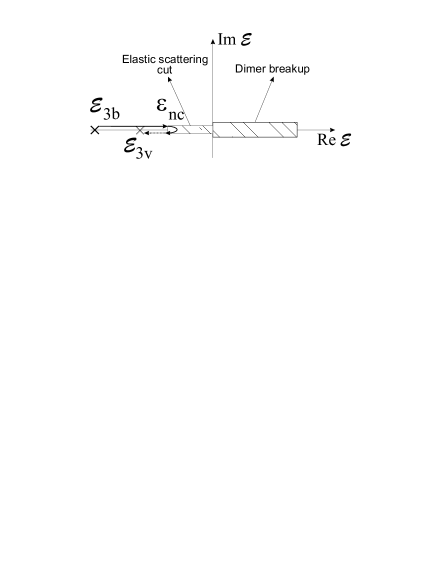
Figure 1: Analytic structure of the $S-$matrix. The energies of the neutron-core (bound system), the three-body bound and the three-body virtual states are, respectively, given by $\varepsilon_{nc}$, ${\cal E}_{3b}$, and ${\cal E}_{3v}$. The arrow passing through the elastic scattering cut shows the trajectory of an $S-$matrix pole to the second Riemann sheet.

Next, we introduce the basic formalism by starting with the coupled spectator functions for a bound three-body system $n-n-c$ ($c\equiv$ ${}^{18}C$ in our specific case). Our units are such that $\hbar=m_{n}=1$, where $m_{n}$ is the mass of the neutron, with the $n-n$, $n-c$ and three-body energies respectively given by $E_{nn}=\hbar^{2}\varepsilon_{nn}/m_{n}$, $E_{nc}=\hbar^{2}\varepsilon_{nc}/m_{n}$, and $E_{3b}=\hbar^{2}{\cal E}_{3b}/m_{n}$, where $n-n$ and $n-c$ refer to virtual and bound subsystems. After partial wave projection, the $\ell$-wave spectator functions $\chi_{n}^{\ell}$ and $\chi_{c}^{\ell}$ (where the subindex $n$ or $c$ indicates the spectator particle), for a bound three-body system, are given by [3]

$${}\chi_{n}^{\ell}(q;{\cal E}_{3b}) = \tau_{nc}(q;{\cal E}_{3b})\int_{0}^{\infty}dkk^{2}\left[K_{2}^{\ell}(q,k;{\cal E}_{3b})\chi_{n}^{\ell}({k};{\cal E}_{3b})+K_{1}^{\ell}(q,k;{\cal E}_{3b})\chi_{c}^{\ell}({k};{\cal E}_{3b})\right],$$ (1)

$${}\chi_{c}^{\ell}({q};{\cal E}_{3b}) = \tau_{nn}(q;{\cal E}_{3b})\int_{0}^{\infty}dkk^{2}\;K_{1}^{\ell}(k,q;{\cal E}_{3b})\chi_{n}^{\ell}({k};{\cal E}_{3b}),\vspace{-.5cm}$$ (2)

where

$$K_{i=1,2}^{\ell}(q,k;{\cal E}_{3b}) \equiv G_{i}^{\ell}(q,k;{\cal E}_{3b})-\delta_{\ell 0}\;G_{i}^{\ell}(q,k;-\mu^{2})$$ (3)

$$G_{i}^{\ell}(q,k;{\cal E}_{3b}) = \int_{-1}^{1}dy\frac{P_{\ell}(y)}{{\cal E}_{3b}-\frac{A+1}{A+A^{i-1}}q^{2}-\frac{A+1}{2A}k^{2}-\frac{kqy}{A^{i-1}}},$$ (4)

$$\tau_{nn}(q;{\cal E}_{3b}) \equiv \frac{-2}{\pi}\left[\sqrt{|\varepsilon_{nn}|}+\sqrt{\frac{A+2}{4A}q^{2}-{\cal E}_{3b}}\right]^{-1},$$ (5)

$$\tau_{nc}(q;{\cal E}_{3b}) \equiv \frac{1}{\pi}\left[\frac{A+1}{2A}\right]^{3/2}\left[\sqrt{|\varepsilon_{nc}|}-\sqrt{\frac{(A+2)}{2(A+1)}q^{2}-{\cal E}_{3b}}\right]^{-1}\;.$$ (6)

In the above, ${\cal E}_{3b}\equiv\varepsilon_{nc}-\frac{A+2}{2(A+1)}\kappa_{b}^{2}$ and $A$ is the mass-number of particle $c$. The absolute value of the momentum of the spectator particle with respect to the center-of-mass (CM) of the other two particles is given by $q\equiv|\vec{q}|$; with $k\equiv|\vec{k}|$ being the absolute value of the relative momentum of these two particles. The $n-n$ virtual state energy is fixed at $E_{nn}=-$143 keV. In Eqs. (1) and (2), we have the Kronecker delta $\delta_{\ell 0}$ ($=1$ for $\ell=0$ and =0 for $\ell\neq 0$) in order to renormalize the equations (using a subtraction procedure) only for the partial wave where such renormalization is necessary, $\ell=0$. In the cases of $\ell>0$, due to the centrifugal barrier, the Thomas collapse is absent and such renormalization is not necessary. In this way, with Eqs. (1) and (2) renormalized, the three-body observables are completely defined by the two-body energy scales, $\varepsilon_{nc}$ and $\varepsilon_{nn}$. Later on, the definitions (3)-(6) will be extended also to unbound systems. The regularization scale $\mu^{2}$, used in the $s-$wave [see Eq. (3)], is chosen to reproduce the three-body ground-state energy of ²⁰C, $E_{0}=-$3.5 MeV [6]. A limit cycle [16, 18] for the scaling function of $s-$wave observables is evidenced when $\mu$ is let to be infinity. We note that, a good description of this limit is already reached in the first cycle [11].

The analytic continuation of the bound three-body system given by (1) and (2) to the second Riemann sheet is performed through the $n-(n-c)$ elastic scattering cut, following Refs. [11, 17, 19]. As we are considering $n-n-c$ nuclei where only the subsystem $n-c$ is bound (“samba-type” nuclei [14, 15]), we have only the $n-c$ cut in the complex energy plane. In order to see how to perform the analytical continuation from the first to the second sheet of the complex energy, let us first consider a complex momentum variable $k_{i}$. As the energies of the two-body sub-systems are fixed and only the $n-c$ subsystem is bound, it is convenient to define this momentum as $k_{i}=\sqrt{\frac{2(A+1)}{A+2}\left({\cal E}_{i}-\varepsilon_{nc}\right)}$. In this case, the bound-state energy $({\cal E}_{i}={\cal E}_{3b})$ is given by $k_{i}={\rm i}\kappa_{b}$, with the virtual state energy (${\cal E}_{i}={\cal E}_{3v}$) given by $k_{i}=-{\rm i}\kappa_{v}$. Next, by removing ${\cal E}_{3b}$ in favor of $k_{i}$ in the bound-state equations (1)-(6), with

$${\bar{\tau}_{nc}}(q;{\cal E})\equiv\frac{-1}{\pi}\left(\frac{A+1}{2A}\right)^{\frac{3}{2}}\left(\sqrt{|\varepsilon_{nc}}|+\sqrt{\frac{(A+2)q^{2}}{2(A+1)}-{\cal E}}\right),$$ (7)

and with $\chi_{c}$ and $\chi_{n}$ redefined as

$$\chi_{c}^{\ell}({q};{\cal E})\equiv h_{c}^{\ell}({q};{\cal E}),\;\;\displaystyle\chi_{n}^{\ell}({q};{\cal E})\equiv h_{n}^{\ell}({q};{\cal E})/{(q^{2}-k_{i}^{2}-i\epsilon)},$$ (8)

we observe that the relevant integrals to be considered have the structure ${\cal I}(k_{i})=\int q^{2}dq\left[{F(q^{2})}/{(k_{i}^{2}-q^{2}+{\rm i}\epsilon)}\right]$ in the first sheet of the complex energy plane. To obtain ${\cal I}(k_{i})$ in the second sheet we need to change the contour of integration, as shown in detail in Ref. [7], such that the value of ${\cal I}(k_{i})$ in the second sheet of the complex energy plane is given by ${\cal I^{\prime}}(k_{i})={\cal I}(k_{i})-{\rm i}\pi k_{i}F(k_{i}^{2}).$ Following this procedure, from Eqs. (1) and (2) we obtain the corresponding equations in the second sheet of the complex energy plane, where for the virtual state energy we have $k_{i}=-{\rm i}\kappa_{v}=\sqrt{\frac{2(A+1)}{A+2}\left({\cal E}_{3v}-\varepsilon_{nc}\right)}$:

$${}h_{n}^{\ell}(q;{\cal E}_{3v})= \frac{2(A+1)}{A+2}{\bar{\tau}_{nc}}(q;{\cal E}_{3v})\left[{\pi}{\kappa_{v}}K_{2}^{\ell}(q,-{\rm i}\kappa_{v};{\cal E}_{3v})h_{n}^{\ell}(-{\rm i}\kappa_{v};{\cal E}_{3v})+\right.$$ (9)

$$+\left.\int_{0}^{\infty}{\hskip-2.84544pt}dkk^{2}{}\left({}K_{1}^{\ell}(q,k;{\cal E}_{3v})h_{c}^{\ell}(k;{\cal E}_{3v})+\frac{K_{2}^{\ell}(q,k;{\cal E}_{3v})\;h_{n}^{\ell}(k;{\cal E}_{3v})}{k^{2}+\kappa_{v}^{2}}{}\right){}\right],$$

$${}h_{c}^{\ell}(q;{\cal E}_{3v})= {}\tau_{nn}(q;{\cal E}_{3v})\left[{\pi}{\kappa_{v}}K_{1}^{\ell}(-{\rm i}\kappa_{v},q;{\cal E}_{3v})h_{n}^{\ell}(-{\rm i}\kappa_{v};{\cal E}_{3v})+\right.$$ (10)

$$+\left.\int_{0}^{\infty}dkk^{2}\;\frac{K_{1}^{\ell}(k,q;{\cal E}_{3v})\;h_{n}^{\ell}(k;{\cal E}_{3v})}{k^{2}+\kappa_{v}^{2}}\right].$$

The above coupled equations, as well as the corresponding coupled equations for bound state, can be written as single-channel equations for $h_{n}^{\ell}$, by defining an effective interaction ${\cal V}$ and considering $I=b,v$:

$${}h_{n}^{\ell}(q;{\cal E}_{3I}) = 2{\kappa_{v}}h_{n}^{\ell}(-{\rm i}\kappa_{v};{\cal E}_{3v}){\cal V}^{\ell}(q,-{\rm i}\kappa_{v};{\cal E}_{3v})\delta_{I,v}+\frac{2}{\pi}\int_{0}^{\infty}{\hskip-2.84544pt}dkk^{2}{\cal V}^{\ell}(q,k;{\cal E}_{3I})\frac{h_{n}^{\ell}(k;{\cal E}_{3I})}{k^{2}+\kappa_{I}^{2}}$$

$${}{\cal V}^{\ell}(q,k;{\cal E}_{3I}) \equiv \pi\frac{(A+1)}{A+2}{\bar{\tau}_{nc}}(q;{\cal E}_{3I})\times$$ (12)

$$\times \left[K_{2}^{\ell}(q,k;{\cal E}_{3I})+\int_{0}^{\infty}dk^{\prime}k^{\prime 2}K_{1}^{\ell}(q,k^{\prime};{\cal E}_{3I})\tau_{nn}(k^{\prime};{\cal E}_{3I})K_{1}^{\ell}(k,k^{\prime};{\cal E}_{3I})\right].$$

The first term in the right-hand-side (rhs) of (Trajectory of neutron$-$neutron$-^{18}C$ excited three-body state), which is non-zero only for the virtual state, corresponds to the contribution of the residue at the pole. The virtual states are limited by the cut of the elastic scattering amplitude in the complex plane, corresponding to the second term in the rhs of Eq. (9). In this case, the cut is given by the zero of the denominator of $G_{2}^{\ell}(q,k;{\cal E}_{3v})$ [See Eq. (4)], where $-1<y<1$ and $q=k=-{\rm i}\kappa_{cut}$. With $|{\cal E}_{3v}|=|\varepsilon_{nc}|+\frac{A+2}{2(A+1)}\kappa_{cut}^{2}$, we obtain the branch points, with the cut given by

$$\frac{2(A+1)}{A+2}|\varepsilon_{nc}|<|{\cal E}_{3v}|<\frac{2(A+1)}{A}|\varepsilon_{nc}|.$$ (13)

For $n-n-^{18}$C ($A=18$), a virtual state energy can be found in the energy interval between the threshold of the elastic scattering and the starting of the above cut (13):

$$|\varepsilon_{nc}|\;<\;|{\cal E}_{3v}|\;<\;1.9\;|\varepsilon_{nc}|\ .$$ (14)

Figure 2: Three-body $n-n-^{18}$C results for the first excited state, with respect to the threshold ($|E_{{}^{20}{\rm C}}-E_{{}^{19}{\rm C}}|$) for varying ¹⁹C binding energies. Three-body bound (virtual) states occur when $|E_{{}^{19}{\rm C}}|$ is approximately smaller (larger) than 170 keV. $s-$wave results (solid line) are also presented in the inset (with dots). Results for the $p-$and $d-$waves, divided by a factor 10, are shown with dashed and dotted lines, respectively.

Figure 2 shows how the absolute value of the first excited three-body state energy with respect to the two-body bound state, $|E-E_{nc}|$, varies when increasing the $n-c$ bound-state energy. In this case, with ¹⁸C being the core, we have ¹⁹C as the two-body bound subsystem. The solid line of Fig. 2 presents the $s-$wave results, with a close focus in the region of the threshold ($E=E_{nc}$) given by the inset figure. Although the Efimov states do not appear in higher partial waves due to the existence of the centrifugal barrier, we have also presented results for the virtual states of $p-$ and $d-$ waves in view of their possible relevance for the elastic $n-^{19}$C low-energy cross-section. Such situation can happen when the $s-$wave virtual state is far from the elastic scattering region.
The results shown in Fig. 2, valid for $n-n-c$ system with $n-c$ bound, together with previous analysis [3, 11], are clarifying that the behavior of Efimov states, when one of the particles have a mass different from the other two, follows the same pattern as found in the case of three equal-mass particles [8, 10]. No resonances were found for Eqs. (9) and (10) in the complex energy plane.
Next, for consistency, we present results for the $s-$wave elastic cross-sections, which are in agreement with the above. The formalism for the partial-wave elastic $n-~{}^{19}$C scattering equations can be obtained from Eqs. (1) and (2), by first introducing the following boundary condition in the full-wave spectator function $\chi_{n}(\vec{q})$:

$$\chi_{n}(\vec{q})\equiv(2\pi)^{3}\delta(\vec{q}-\vec{k}_{i})+4\pi\frac{h_{n}(\vec{q};{\cal E}(k_{i}))}{q^{2}-k_{i}^{2}-{\rm i}\epsilon},$$ (15)

where $h_{n}(\vec{q};{\cal E}(k_{i}))$ is the scattering amplitude, and the on-energy-shell incoming and final relative momentum are related to the three-body energy ${\cal E}_{i}\equiv{\cal E}(k_{i})$ by $k_{i}\equiv|\vec{k}_{i}|=|\vec{k}_{f}|=\sqrt{[2(A+1)/(A+2)]\left({\cal E}_{i}-\varepsilon_{nc}\right)}.$ With the same formal expressions (7) and (6) for $\bar{\tau}_{nc}$ and $\tau_{nn}$, by using the definition (Trajectory of neutron$-$neutron$-^{18}C$ excited three-body state), the partial-wave scattering equation can be cast in the following single channel Lippmann-Schwinger-type equation for $h_{n}^{\ell}$:

$$h_{n}^{\ell}(q;{\cal E}_{i})={\cal V}^{\ell}(q,k_{i};{\cal E}_{i})+\frac{2}{\pi}\int_{0}^{\infty}dkk^{2}\;\frac{{\cal V}^{\ell}(q,k;{\cal E}_{i})\;h_{n}^{\ell}(k;{\cal E}_{i})}{k^{2}-k_{i}^{2}-{\rm i}\epsilon}.$$ (16)

Virtual states and resonances correspond to poles of the scattering matrix on unphysical sheets. So, the most natural method to look for them is to perform an analytically continuation of the scattering matrix to the unphysical sheet. For that one needs prior knowledge about the analytic properties of the kernel of the integral equation, as well as the scattering matrix properties on the unphysical sheet of the complex energy plane. Although such properties are easy to derive in simple cases, they can be difficult to obtain in more complex situations, which can put some restriction on the approach.

For the numerical treatment of Eq. (16), we consider the approach developed in [8] to find virtual states and resonances on the second energy sheet associated with the lowest scattering threshold. Such approach does not require prior knowledge of the analytic properties of the scattering matrix on the unphysical sheet. The solution of the scattering equation is written in a form where the analytic structure in energy is clearly exhibited. Then, it is analytically continued to the unphysical sheet. The method relies on the calculation of an auxiliary (resolvent) function [20], which has an integral structure similar to the original scattering equation, but with a weaker kernel due to a subtraction procedure at an arbitrary fixed point $\bar{k}_{i}$. For real positive energies, this subtraction point $\bar{k}_{i}$ is identified with $k_{i}$, such that the corresponding integral equation does not have the two-body unitarity cut. For non-real or negative energies, $\bar{k}_{i}$ can be any arbitrary positive real number. For convenience, $\bar{k}_{i}=|k_{i}|$. The final solution is obtained by evaluating certain integrals over the auxiliary function. In case of scattering solutions, the two-body unitarity cut is introduced through these integrals. In the present case, we have the following integral equation for the auxiliary function $\Gamma$, and the corresponding solution for $h_{n}^{\ell}(q;{\cal E}_{i})$:

$${\Gamma_{n}^{\ell}}(q,k_{i};{\cal E}_{i}) = {\cal V}^{\ell}(q,k_{i};{\cal E}_{i})+\frac{2}{\pi}\int_{0}^{\infty}dk\left[k^{2}{\cal V}^{\ell}(q,k;{\cal E}_{i})-\bar{k}_{i}^{2}{\cal V}^{\ell}(q,k_{i};{\cal E}_{i})\right]\frac{{\Gamma_{n}^{\ell}}(k,k_{i};{\cal E}_{i})}{k^{2}-k_{i}^{2}},$$

$${h_{n}^{\ell}}(q;{\cal E}_{i}) = {\Gamma_{n}^{\ell}}(q,k_{i};{\cal E}_{i})+{\Gamma_{n}^{\ell}}(q,\bar{k}_{i};{\cal E}_{i})\frac{\displaystyle\frac{2}{\pi}{\bar{k}_{i}^{2}}\int_{0}^{\infty}dk\;\frac{{\Gamma_{n}^{\ell}}(k,k_{i};{\cal E}_{i})}{k^{2}-k_{i}^{2}-{\rm i}\epsilon}}{\displaystyle 1-\frac{2}{\pi}{\bar{k}_{i}^{2}}\int_{0}^{\infty}dk\;\frac{{\Gamma_{n}^{\ell}}(k,{\bar{k}_{i}};{\cal E}_{i})}{k^{2}-k_{i}^{2}-{\rm i}\epsilon}}.$$ (17)

For the on-shell scattering amplitude, we have

$$h_{n}^{\ell}(k_{i};{\cal E}_{i})=[1/{\Gamma_{n}^{\ell}}(k_{i},k_{i};{\cal E}_{i})-{\cal J}]^{-1}$$ (18)

$${\cal J}\equiv\frac{2}{\pi}k_{i}^{2}\int_{0}^{\infty}dk\;\frac{\left[{\Gamma_{n}^{\ell}}(k,k_{i};{\cal E}_{i})/{\Gamma_{n}^{\ell}}(k_{i},k_{i};{\cal E}_{i})-1\right]}{k^{2}-k_{i}^{2}}+{\rm i}k_{i}$$

In order to obtain the bound and virtual energy states, two independent procedures have been used. The first one, by solving directly the homogeneous coupled equations (1), (2), (9) and (10), looking for zeros of the corresponding determinants. The other one, by verifying the position of the poles in the complex energy plane of the scattering amplitude, $h_{n}^{\ell}(k_{i};{\cal E}_{i})$, given by Eq. (18) and corresponding analytic extension to the second Riemann sheet. In this second approach, we solve the corresponding inhomogeneous equation with on-energy-shell momentum $k_{i}=+{\rm i}\kappa_{b}$ (bound state, ${\cal E}_{i}=-|{\cal E}_{3b}|$) and $k_{i}=-{\rm i}\kappa_{v}$ (virtual state, ${\cal E}_{i}=-|{\cal E}_{3v}|$)[8].

By comparing the results of both approaches, we checked that they give consistent results. However, for numerical stability and accuracy of the results, particularly in the case of the search for Efimov states, when the absolute values of the energies are very close to zero, the second approach is by far much better.

Figure 3: $n-^{19}$C elastic cross sections (in barns) versus the CM kinetic energies [Eq. (19) with A=18], for different ¹⁹C bound energies. In the left-hand-side frame we show results for two cases that generate three-body energies close to the threshold: $E_{{}^{19}{\rm C}}=-$150 keV (main figure) and $-$180 keV (inset), producing respectively three-body bound and virtual states. Solid-line are obtained from (16), with dashed-line from (20). In the rhs we have results for $E_{{}^{19}{\rm C}}=-$500 keV.

Results for the total $n-^{19}$C elastic cross-sections, obtained from ${d\sigma}/{d\Omega}=|h_{n}(\vec{k}_{f};{\cal E}_{i})|^{2}$, refering to bound or virtual states $E^{*}$, are presented in Fig. 3 as functions of the CM kinetic energy,

$${\cal K}(k_{i})\equiv{[(A+2)\;k_{i}^{2}]}/{[2(A+1)]}=E(k_{i})-E_{nc}.$$ (19)

Although each higher partial $\ell-$wave have a virtual state, below the breakup the cross-section is completely dominated by the $s-$wave [19]. In the frame shown in the left-hand-side, we have two cases of energies close to the scattering threshold: $n-{{}^{18}{\rm C}}$ bound at $-$150 keV, giving an excited Efimov bound state with $E^{*}=-$150.12 keV; and $n-{{}^{18}{\rm C}}$ bound at $-$180 keV, producing a virtual state with $E^{*}=-$180.12 keV. In both two cases the cross-section has a huge peak at zero energy due to the presence of the nearby pole. For comparison, we also show (with dashed-line) the results obtained from the following effective range expansion (approximately valid for small $k_{i}$ near the elastic scattering threshold):

$$\sigma(k_{i})=\frac{4\pi\hbar^{2}}{\displaystyle{1.9m_{n}}\left(E_{nc}-E^{*}\right)+\hbar^{2}k_{i}^{2}}\simeq\frac{\displaystyle 2741\;{\rm keV}}{E(k_{i})-E^{*}}\;{\rm barn},$$ (20)

where we have used $A=$18, $\hbar^{2}/m_{n}=$414.42 keV barn and Eq. (19). The case not so close to the threshold (where Eq.(20) fails) is shown in rhs for $E_{nc}=-$500 keV, with ²⁰C virtual energy $E^{*}=-$568.73 keV.
The proximity of an Efimov state (bound or virtual) to the neutron and neutron-core elastic scattering makes the cross-section extremely sensitive to the corresponding $S$-matrix pole. We remark that if it will be possible to dissociate a “samba-type” halo nuclei, like ²⁰C, and measure the correlation function in the two-body channel corresponding to a neutron and a bound $n-c$ system for small relative momentum, the information on the final state interaction as well as the halo structure will be clearly probed, as the counterpart seen in the $n-n$ correlation in the breakup of Borromean nuclei [21].

In conclusion, we analyzed the three-body halo system $n-n-^{18}$C, where two pairs ($n-^{18}$C) are bound, and the remaining pair $n-n$ has a virtual-state. We study the trajectory of three-body Efimov states in the complex energy plane. As shown, the energy of an excited Efimov state varies from a bound to a virtual state as the binding energy of the subsystem $n-^{18}$C is increased, while keeping fixed the ²⁰C ground-state energy and the virtual energy of the remaining pair ($n-n$). In our approach we applied a renormalized zero-range model, valid in the limit of large scattering lengths. Considering that low-energy correlations, as the one represented by the Phillips line [22] (correlation between triton and doublet neutron-deuteron scattering length), are well reproduced by zero-range potentials [23], the present conclusions should remain valid also for finite two-body interactions when the scattering length is much larger than the potential range. On the numerical analysis, we should remark that we have considered two approaches that give consistent results for bound and virtual state energies. In the case of Efimov physics, where the poles are very close to zero, the method considered in Ref. [8] was found to give solutions with much better stability and accuracy in the scattering region than by using a contour deformation technique.

The present results are extending to $n-n-$core systems the long ago conclusion reached for three equal-mass particles [8, 10]: by increasing the binding energy of the $n-$core subsystem, an excited weakly-bound three-body Efimov state moves to a virtual one and will not become a resonance. From Fig. 3, one can also observe that the $n-^{19}$C elastic cross-sections at low energies present a smooth behavior dominated by the $S-$matrix pole corresponding to a bound or virtual three-body state. In contrast with the above conclusion applied to system where $n-c$ is bound, we should observe that it was also verified that an excited Efimov state can go from a bound to a resonant state (instead of virtual state) in case of Borromean systems (with all the subsystems unbound), when the absolute value of a virtual-state energy for the $n-c$ system is increased [12]. Actually, it should be of interest to extend the present analysis of the trajectory of Efimov states to other possible two-body configurations, with different mass relations of three-particle systems.

In view of the exciting possibilities of varying the two-body interaction, it can be of high interest the results of the present study to analyze properties of three-body systems in ultracold atomic experiments. For negative scattering lengths the Efimov state goes to a continumm resonance when $|a|$ is decreased, as observed by the change of resonance peak in the three-body recombination to deeply bound states towards smaller values of $|a|$ by raising the temperature [24]. Alternatively, for positive $a$ the recombination rate has a peak when the Efimov state crosses the threshold and turns into a virtual state when decreasing $a$. A dramatic effect will appear in the atom-dimer scattering rate when the cross-section is dominated by the $S$-matrix pole near the scattering threshold. We foreseen that the coupling between atom and molecular condensate will respond strongly to the crossing of the triatomic bound state to a virtual one by changing $a$. Determined by the dominance of the coupled channel interaction, new condensate phases of the atom-molecule gas are expected. The proximity of the virtual trimer state to the physical region, implying in a large negative atom-dimer scattering length, will warrant stability to both condensates, while the positive atom-dimer scattering length, due to a trimer bound state near threshold, make possible the collapse of the condensed phases. Indeed, the occurrence of some interesting effects in the condensate due to Efimov states near the scattering threshold have already been discussed in Refs. [25]. We hope these exciting new consequences of Efimov physics can be explored experimentally in the near future.

LT thanks Prof. S.K. Adhikari for helpful suggestions. We also thank Fundação de Amparo à Pesquisa do Estado de São Paulo and Conselho Nacional de Desenvolvimento Científico e Tecnológico for partial support.

References

- [1] V. Efimov, Phys. Lett. B 33 (1970) 563.
- [2] T. Kraemer et al, Nature 440 (2006) 315.
- [3] A. E. A. Amorim, T. Frederico and L. Tomio Phys. Rev. C 56 (1997) R2378.
- [4] V. Arora, I. Mazumdar, V. S. Bhasin, Phys. Rev. C 69 (2004) 061301(R); I. Mazumdar, A. R. P. Rau, V. S. Bhasin, Phys. Rev. Lett. 97 (2006) 062503.
- [5] A. S. Jensen, K. Riisager, D. V. Fedorov, E. Garrido, Rev. Mod. Phys. 76 (2004) 215.
- [6] G. Audi, A. H. Wapstra, and C. Thibault, Nucl. Phys. A 729 (2003) 337.
- [7] S. K. Adhikari, A. C. Fonseca, and L. Tomio, Phys. Rev. C 26 (1982) 77.
- [8] S. K. Adhikari and L. Tomio, Phys. Rev. C 26 (1982) 83.
- [9] R. D. Amado, Phys. Rev. 132 (1963) 485.
- [10] R. D. Amado and J. V. Noble, Phys. Rev. D 5 (1972) 1992; S. K. Adhikari and R. D. Amado, Phys. Rev. C 6 (1972) 1484.
- [11] M. T. Yamashita, T. Frederico, A. Delfino, L. Tomio, Phys. Rev. A 66 (2002) 052702.
- [12] F. Bringas, M. T. Yamashita, T. Frederico, Phys. Rev. A 69 (2004) 040702(R).
- [13] M. T. Yamashita, T. Frederico and L. Tomio, submitted to Phys. Rev. Lett.
- [14] M. T. Yamashita, T. Frederico, L. Tomio, Nucl. Phys. A 735 (2004) 40.
- [15] M. T. Yamashita, T. Frederico, M. S. Hussein, Mod. Phys. Lett. A 21 (2006) 1749.
- [16] E. Braaten and H.-W. Hammer, Phys. Rep. 428 (2006) 259.
- [17] W. Glöckle, Phys. Rev. C 18 (1978) 564; Walter Glöckle, The Quantum Mechanical Few-Body Problem (Springer-Verlag, Berlin, 1983).
- [18] S. D. Glazek, K. G. Wilson, Phys. Rev. Lett. 89 (2002) 230401; R. Mohr, R. Furnstahl, H. Hammer, R. Perry, and K. Wilson, Ann. of Phys. 321 (2005) 225.
- [19] A. Delfino, T. Frederico, M. S. Hussein and L. Tomio, Phys. Rev. C 61 (2000) 051301(R).
- [20] L. Tomio and S. K. Adhikari, Phys. Rev. C 22 (1980) 28; 22 (1980) 2359; 24 (1981) 43. See refs. therein for other similar approaches. For bound-states, see S. K. Adhikari and L. Tomio, Phys. Rev. C 24 (1981) 1186.
- [21] M. Petrascu, et al., Phys. Rev. C 73 (2006) 057601; M. T. Yamashita, T. Frederico, L. Tomio, Phys. Rev. C 72 (2005) 011601(R).
- [22] A. C. Phillips, Nucl. Phys. A 107 (1968) 209.
- [23] S. K. Adhikari and J.R.A. Torreão, Phys. Lett. B 132 (1983) 257; D.V. Fedorov and A.S. Jensen, Nucl. Phys. A 697 (2002) 783; P. F. Bedaque, U. van Kolck, Ann. Rev. Nucl. Part. Sci. 52 (2002) 339.
- [24] M. T. Yamashita, T. Frederico, L. Tomio, Phys. Lett. A 363 (2007) 468.
- [25] A. Bulgac, Phys. Rev. Lett. 89 (2002) 050402; B.J. Cusack, T.J. Alexander, E.A. Ostrovskaya, and Y.S. Kivshar, Phys. Rev. A 65 (2002) 013609; E. Braaten, H.-W. Hammer, and T. Mehen, Phys. Rev. Lett. 88 (2002) 040401; E. Braaten, H.-W. Hammer, and M. Kusunoki, Phys. Rev. Lett. 90 (2003) 170402.