On the existence of chaotic circumferential waves in spinning disks

Abstract

We use a third-order perturbation theory and Melnikov’s method to prove the existence of chaos in spinning circular disks subject to a lateral point load. We show that the emergence of transverse homoclinic and heteroclinic points respectively lead to a random reversal in the traveling direction of circumferential waves and a random phase shift of magnitude $\pi$ for both forward and backward wave components. These long-term phenomena occur in imperfect low-speed disks sufficiently far from fundamental resonances.

Transversal vibration modes of hard disk drives (HDDs) are excited by the lateral aerodynamic force of the magnetic head. Previous works RM01 ; JA1 revealed that chaotic orbits are inevitable ingredients of phase space flows when the lateral force is large, or the disk is rotating near the critical resonant speed. For low-speed disks, however, an adiabatic invariant (a first integral) was found JA1 using a first-order averaging based on canonical Lie transforms. According to the first-order theory, regular vibrating modes of imperfect, low-speed disks are independent of the angular velocity of the disk, $\Omega_{0}$. In such a circumstance, the speed of circumferential waves is the natural frequency of the lateral mode, $\omega$, derived from linear vibration analysis. HDDs are usually operated with angular velocities smaller than $\omega$ (safely below resonance). Moreover, the magnitude of the lateral force $F$ is very small. Given these conditions, we show that it is impossible to continue the Lie perturbation scheme JA1 up to terms of arbitrary order and remove the time variable $t$ from the Hamiltonian. In fact, due to the special forms of nonlinearities in the dynamical equations of spinning disks, one can not remove $t$ from third-order terms. Subsequent application of a second-order Melnikov theory reveals that transverse homoclinic and heteroclinic points do exist for all $F,\Omega_{0}\not=0$. This implies chaos, or equivalently, non-integrability of governing equations.

I Introduction

Dynamics of continuum media, like fluids, rods, plates and shells is usually formulated as a system of partial differential equations (PDEs) for physical quantities in terms of the spatial coordinates x and the time $t$ as

$${\cal L}(\textbf{u})=0.$$ (1)

Here ${\cal L}$ is a nonlinear operator and $\textbf{u}(\textbf{x},t)$ is the vector of dependent variables. When the boundary conditions are somehow simple, approximate variational methods based on modal decomposition and Galerkin’s projection Reddy86 can be used to reduce the order of governing equations. These methods begin with solving an auxiliary eigenvalue problem, which is usually the variational field equation $\delta{\cal L}(\textbf{u},\Lambda)=0$, and build some complete basis set $\textbf{U}_{\textbf{k}}(\textbf{x},\Lambda_{\textbf{k}})$ for expanding $\textbf{u}(\textbf{x},t)$ in the spatial domain. Here $\Lambda_{\textbf{k}}$ is an eigenvalue, which is characterized by the vectorial index k. Each $\textbf{U}_{\textbf{k}}$ is called an eigenmode or a shape function. Such a basis set should preferably satisfy boundary conditions and be orthogonal.

Once a complete basis set is constructed, one may suppose a solution of the form

$$\textbf{u}(\textbf{x},t)=\sum_{\textbf{k}}\textbf{V}_{\textbf{k}}(t)\cdot\textbf{U}_{\textbf{k}}(\textbf{x},\Lambda_{\textbf{k}}).$$ (2)

Substituting from (2) into (1) and taking the inner product

$$\int{\cal L}(\textbf{u})\cdot\textbf{U}_{\textbf{k}^{\prime}}(\textbf{x}){\rm d}\textbf{x}=0,$$ (3)

leaves us with a system of nonlinear ordinary differential equations (ODEs) for the amplitude functions $\textbf{V}_{\textbf{k}}(t)$. The evolution of the reduced ODEs shows the interaction of different modes and their influence on the development of spatiotemporal patterns.

In a series of papers, Raman and Mote RM01 ; RM99 used the modal decomposition method to investigate transversal oscillations of spinning disks whose deformation field is described in terms of the displacement vector $(u,v,w)$ with $u$ and $v$ being the in-plane components. The most important application of the spinning disk problem is in design, fabrication and control of HDDs. The governing PDEs for the evolution of displacement components were first derived by Nowinski N64 and reformulated more recently by Baddour and Zu BZ01 . Let us define $(R,\phi)$ as the usual polar coordinates. For a rotating disk with the angular velocity $\Omega_{0}$, Nowinski’s theory assumes that the in-plane inertias $(u,v)\Omega_{0}^{2}$, $2\Omega_{0}(u_{,t},v_{,t})$ and $(u_{,tt},v_{,tt})$ are ignorable against $R\Omega_{0}^{2}$. This is a rough approximation for high-speed disks and one needs to use the complete set of equations as Baddour and Zu BZ01 suggest. Nowinski’s theory, however, has its own advantages (like the existence of a stress function) that facilitate the study of the most important transversal modes. In low-speed disks, or disks with high flexural rigidity, one has $\Omega_{0}\ll\omega$. Hence, it is legitimate to apply Nowinski’s governing equations in such systems.

In this paper we analytically prove the existence of chaos, and therefore, non-integrability of the reduced ODEs that govern the double-mode oscillations of imperfect spinning disks. We investigate low-speed disks subject to a lateral point force exerted by the magnetic head. The lateral force in HDDs is very small and its origin is the aerodynamic force due to air flow in the gap between the disk and the head. We show that chaotic circumferential waves dominate some zones of the phase space over the time scale $t\sim{\cal O}(\epsilon^{-3})$ with $\epsilon$ being a small perturbation parameter. This indicates very slow evolution of random patterns, and the practical difficulties of their identification.

The paper is organized as follows. In §II, we present the Hamiltonian function in terms of Deprit’s D91 Lissajous variables. In §III, we use a canonical perturbation theory D69 ; DE91 to eliminate the fast anomaly $l$ from the Hamiltonian. The action associated with $l$ then becomes an adiabatic invariant. Transversal intersections of destroyed invariant manifolds, and therefore, non-integrability of the normalized equations, is proved by a second-order Melnikov method in §IV. We present a complete classification of circumferential waves in §V and end up the paper with concluding remarks in §VI.

II Problem formulation

Let us assume $U_{m}(R)$ as an orthogonal basis set that represents the disk deformation in the radial direction. The index $m$ stands for the number of radial nodes that $U_{m}(R)$ has. According to Raman and Mote’s RM01 treatment of imperfect disks, the following choice of the transversal displacement field

$$w(R,\phi,t)=U_{m}(R)[x(t)\cos n\phi+y(t)\sin n\phi],$$ (4)

reduces Nowinski’s governing equations to a system of ODEs for the amplitude functions $x(t)$ and $y(t)$ as

$$\ddot{x}+\lambda^{2}x+\epsilon\gamma\left(x^{2}+y^{2}\right)x\! = \!\epsilon F\cos(n\Omega_{0}t),$$ (5a)

$$\ddot{y}+\omega^{2}y+\epsilon\gamma\left(x^{2}+y^{2}\right)y\! = \!\epsilon F\sin(n\Omega_{0}t),$$ (5b)

where $\lambda$, $\omega$ and $\gamma$ are constant parameters that depend on the geometry and material of the disk. $\epsilon$ is a small perturbation parameter, $F$ is the weighted integral of the lateral point force, and $\Omega_{0}$ is the angular velocity of the disk.

We suppose small deviations from perfect disks and write the constant parameter of (5) as $\lambda^{2}/\omega^{2}=1+\epsilon\eta$. We also define $n\Omega_{0}=\epsilon\Omega$ with ${\cal O}(\Omega)\sim{\cal O}(\omega)$. Denoting $(p_{x},p_{y})$ as the momenta conjugate to $(x,y)$, it can be verified that equations (5) are derivable from the Hamiltonian function

$$H = \frac{1}{2}\left(p_{x}^{2}+p_{y}^{2}\right)+\frac{1}{2}\omega^{2}\left(x^{2}+y^{2}\right)+\epsilon\Big{[}\frac{\eta}{2}\omega^{2}x^{2}$$ (6)

$$+ \Omega P\!+\!\frac{\gamma}{4}\left(x^{2}+y^{2}\right)^{2}-F\left(x\cos p+y\sin p\right)\Big{]}.$$

We have introduced the action $P$ and its conjugate angle $p=\epsilon\Omega t$ to make our equations autonomous, which is a preferred form for the application of canonical perturbation theories. The extended phase space has now dimension six. Dynamics generated by (6) is better understood after carrying out a canonical transformation $(x,y,p_{x},p_{y})\rightarrow(l,g,L,G)$ to the space of Lissajous variables D91 so that

$$x = s\cos(g+l)-d\cos(g-l),$$ (7a)

$$y = s\sin(g+l)-d\sin(g-l),$$ (7b)

$$p_{x} = -\omega\left[s\sin(g+l)+d\sin(g-l)\right],$$ (7c)

$$p_{y} = \omega\left[s\cos(g+l)+d\cos(g-l)\right],$$ (7d)

$$s = \sqrt{{L+G\over 2\omega}},~{}~{}d=\sqrt{{L-G\over 2\omega}},~{}~{}L\geq 0,~{}~{}|G|\leq L.$$

In the space of Lissajous variables, the Hamiltonian defined in (6) becomes

$$H = H_{0}(L)+\epsilon H_{1}(l,g,p,L,G,P),$$ (8)

$$H_{0} = \omega L,$$

$$H_{1} = \Omega P-F\left[s\cos(g+l-p)-d\cos(g-l-p)\right]$$

$$+ {\gamma\over 4}\left[(s^{2}+d^{2})-2sd\cos(2l)\right]^{2}$$

$$+ {\eta\omega^{2}\over 4}\Big{[}(s^{2}+d^{2})+s^{2}\cos(2g+2l)-2sd\cos(2g)$$

$$+ d^{2}\cos(2g-2l)-2sd\cos(2l)\Big{]}.$$

From (8) we conclude that $l$ is the fast angle, and $g$ and $p$ are the slow ones. Therefore the long-term behavior of the flows generated by (8) can be analyzed by averaging $H$ over $l$. After removing $l$, its corresponding action $L$ will be a constant of motion for the flows generated by the averaged Hamiltonian $\langle H\rangle_{l}$, and the phase space dimension reduces from 6 to 4.

III Canonical third-order averaging

In order to average $H$ over $l$, we use the normalization procedure of Deprit and Elipe DE91 . Denoting $X\equiv(l,g,p)$ and $Y\equiv(L,G,P)$, we define a Lie transformation $(l,g,p,L,G,P)\rightarrow(\bar{l},\bar{g},\bar{p},\bar{L},\bar{G},\bar{P})$ as

$$X=E_{W}(\bar{X}),~{}~{}Y=E_{W}(\bar{Y}),$$ (9)

so that the Hamiltonian function in terms of the new variables, $K\equiv\langle H\rangle_{l}$, does not depend on $\bar{l}$. $E_{W}$ is the Lie transform generated by the function $W$ and it is defined as

$$E_{W}(\bar{Z}) = \bar{Z}+(\bar{Z};W)+\frac{1}{2!}((\bar{Z};W);W)$$ (10)

$$+ \frac{1}{3!}(((\bar{Z};W);W);W)+\cdots.$$

In this equation, $(f_{1};f_{2})$ denotes the Poisson bracket of $f_{1}$ and $f_{2}$ over the $(\bar{l},\bar{g},\bar{p},\bar{L},\bar{G},\bar{P})$-space. We expand the generating function $W$ as

$$W=\epsilon W_{1}+\frac{\epsilon^{2}}{2!}W_{2}+\cdots,$$ (11)

and specify the averaged, target Hamiltonian $K=K(\bar{g},\bar{p},\bar{L},\bar{G},\bar{P})$ as the series DE91

$$K=K_{0}+\epsilon K_{1}+\frac{\epsilon^{2}}{2!}K_{2}+\frac{\epsilon^{3}}{3!}K_{3}+\cdots,$$ (12)

with

$$K_{0}\!\! = \!\!\omega\bar{L},$$ (13a)

$$K_{1}\!\! = \!\!\frac{1}{2\pi}\int^{2\pi}_{0}H_{1}{\rm d}\bar{l},$$ (13b)

$$K_{2}\!\! = \!\!\frac{1}{2\pi}\int^{2\pi}_{0}[2(H_{1};W_{1})+((H_{0};W_{1});W_{1})]{\rm d}\bar{l},$$ (13c)

$$K_{3}\!\! = \!\!\frac{1}{2\pi}\int^{2\pi}_{0}\Big{[}3(H_{1};W_{2})+3((H_{1};W_{1});W_{1})$$ (13d)

$$+ \!\!2((H_{0};W_{2});W_{1})+((H_{0};W_{1});W_{2})$$

$$+ \!\!(((H_{0};W_{1});W_{1});W_{1})\Big{]}{\rm d}\bar{l}.$$

$W_{1}$ and $W_{2}$ are determined through solving the following differential equations

$$\omega\frac{\partial W_{1}}{\partial\bar{l}}\!\!\! = \!\!H_{1}(\bar{l},\bar{g},\bar{p},\bar{L},\bar{G},\bar{P})\!-\!K_{1}(\bar{g},\bar{p},\bar{L},\bar{G},\bar{P}),$$ (14a)

$$\omega\frac{\partial W_{2}}{\partial\bar{l}}\!\!\! = \!\!2(H_{1};W_{1})+((H_{0};W_{1});W_{1})-K_{2}.$$ (14b)

By substituting from (14) into (13) and evaluating the integrals, one finds the explicit form of the new Hamiltonian $K$, which has been given in Appendix A up to the third-order terms.

Once $\bar{l}$ is removed from the Hamiltonian, $\bar{L}$ becomes an integral of motion. The slow dynamics of the system is thus governed by the flows in the $(\bar{g},\bar{G})$-space. We introduce the slow time $\tau=\bar{p}/\Omega$, ignore the fourth-order terms in $\epsilon$, and obtain the following differential equations for the dynamics of $(\bar{g},\bar{G})$

$$\frac{{\rm d}\bar{g}}{{\rm d}\tau}\!\! = \!\!\frac{\partial K}{\partial\bar{G}}=f_{1}(\bar{g},\bar{G})+\epsilon h_{1}(\bar{g},\bar{G},\epsilon,\tau),$$ (15a)

$$\frac{{\rm d}\bar{G}}{{\rm d}\tau}\!\! = \!\!-\frac{\partial K}{\partial\bar{g}}=f_{2}(\bar{g},\bar{G})+\epsilon h_{2}(\bar{g},\bar{G},\epsilon,\tau),$$ (15b)

where

$$f_{1}\!\! = \!\!d_{6}+d_{1}\cos(2\bar{g}),~{}~{}f_{2}=e_{1}\sin(2\bar{g}),$$

$$h_{1}\!\! = \!\!d_{7}+d_{2}\cos(2\bar{g})$$

$$+ \!\!\epsilon[d_{8}+d_{3}\cos(2\bar{g})+d_{4}\cos(4\bar{g})+d_{5}\cos(2\bar{g}-2\Omega\tau)],$$

$$h_{2}\!\! = \!\!e_{2}\sin(2\bar{g})$$ (16)

$$+ \!\!\epsilon[e_{3}\sin(2\bar{g})+e_{4}\sin(4\bar{g})+e_{5}\sin(2\bar{g}-2\Omega\tau)].$$

In these equations, $d_{i}$ ($i=1,\cdots,8$) and $e_{j}$ ($j=1,\cdots,5$) are functions of $\bar{L}$ and $\bar{G}$ (see Appendix A). It is remarked that the action $\bar{P}$ appears only in $K_{1}$ via the term $\Omega\bar{P}$. It then disappears in the normalized equations (15) after taking the partial derivatives of $K$ with respect to $\bar{g}$ and $\bar{G}$. The partial derivative of $K$ with respect to $\bar{P}$ determines the evolution of $\bar{p}$, which is in accordance with the simple linear law $\bar{p}(\tau)=\Omega\tau+\bar{p}(0)$. The dynamics of $\bar{P}$ itself is governed by

$$\frac{{\rm d}\bar{P}}{{\rm d}\tau}=-\frac{\partial K}{\partial\bar{p}}=-\frac{1}{\Omega}\frac{\partial}{\partial\tau}K(\bar{g},\bar{G},\tau).$$ (17)

One may integrate (17) to obtain $\bar{P}(\tau)$ once equations (15) are solved. The behavior of $\bar{P}$ is thus inherited from $\bar{g}(\tau)$ and $\bar{G}(\tau)$.

IV The Melnikov Function

There are few analytical methods in the literature for the detection of chaos in perturbed Hamiltonian systems M63 ; Ch79 . Melnikov’s M63 method is the most powerful technique when the governing equations take the form

$$\frac{{\rm d}\textbf{x}}{{\rm d}\tau}=\textbf{f}(\textbf{x})+\epsilon\textbf{h}(\textbf{x},\epsilon,\tau),~{}~{}\textbf{x}\in\mathbb{R}^{2},$$ (18)

so that the unperturbed system ${\rm d}\textbf{x}/{\rm d}\tau=\textbf{f}(\textbf{x})$ is integrable and possesses a homoclinic (heteroclinic) orbit $\textbf{q}_{\rm h}(\tau)$ to a hyperbolic saddle point, and $\textbf{h}(\textbf{x},\epsilon,\tau)$ is $T$-periodic in $\tau$. The occurrence of chaos is examined by the Melnikov function

$$M(\tau_{0},\epsilon)=\epsilon M_{1}(\tau_{0})+\epsilon^{2}M_{2}(\tau_{0})+\ldots,$$ (19)

where $M_{k}(\tau_{0})$ denotes the $k$th-order Melnikov function. Assume that $M_{i}(\tau_{0})$ is the first nonzero term, i.e., $M_{k}(\tau_{0})\equiv 0$ for $1\leq k\leq i-1$. If $M_{i}(\tau_{0})$ has simple zeros, then, for sufficiently small $\epsilon$, the system (18) has transverse homoclinic (heteroclinic) orbits, which imply chaos due to the Smale-Birkhoff homoclinic theorem GH83 . The first-order term in (19) is determined by the classical formula

$$M_{1}(\tau_{0})=\int^{+\infty}_{-\infty}{\bf{f}}\left({\bf{q}}_{\rm h}\left(\tau\right)\right)\wedge{\bf{h}}\left({\bf{q}}_{\rm h}\left(\tau\right),0,\tau+\tau_{0}\right)\rm{d}\tau,$$ (20)

where the wedge operator $\wedge$ is defined as $\textbf{f}\wedge\textbf{h}=f_{1}h_{2}-f_{2}h_{1}$. Although the Hamiltonian equations (15) have a suitable form for the application of Melnikov’s method, they are autonomous up to the first-order terms in $\epsilon$. Consequently, $M_{1}(\tau_{0})$ vanishes identically for all $\tau_{0}\in[0,T]$. We thus need to investigate the second-order Melnikov function. For doing so, we begin with solving the unperturbed system

$$\frac{{\rm d}\bar{g}}{{\rm d}\tau} = \frac{\partial K_{1}}{\partial\bar{G}}=f_{1}(\bar{g},\bar{G}),$$ (21a)

$$\frac{{\rm d}\bar{G}}{{\rm d}\tau} = -\frac{\partial K_{1}}{\partial\bar{g}}=f_{2}(\bar{g},\bar{G}),$$ (21b)

along homoclinic (heteroclinic) orbits. Jalali and Angoshtari JA1 showed that for $\bar{L}>\eta\omega^{3}/\gamma$, equations (21) have hyperbolic stationary points at $S_{0}\equiv(\bar{g}_{0},\bar{G}_{0})=(-\pi,0)$, $S_{2}\equiv(\bar{g}_{2},\bar{G}_{2})=(0,0)$, and $S_{4}\equiv(\bar{g}_{4},\bar{G}_{4})=(\pi,0)$. The implicit equation of the invariant manifolds that terminate at the saddle points are

$$\cos[2\bar{g}_{\rm h}(\tau)]=\left[\bar{L}-\frac{\gamma}{2\eta\omega^{3}}\bar{G}_{\rm h}^{2}(\tau)\right]\left[\bar{L}^{2}-\bar{G}_{\rm h}^{2}(\tau)\right]^{-1/2}.$$ (22)

   

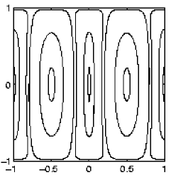
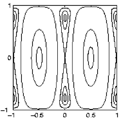
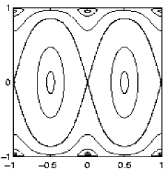
Figure 1: Possible topologies of the phase space flows of the averaged system for $F=0$. In all panels the horizontal axis indicates $\bar{g}/\pi$ and the vertical axis indicates $\bar{G}/\bar{L}$. In the first topology (left panel), all stationary points are of center type. In the second topology (middle panel) two new centers, with non-zero $\bar{G}$-coordinates, have emerged for $\bar{g}=\pm n\pi$ ($n=0,1$) and symmetrical homoclinic loops (thick lines) connect saddle points to themselves. In the third topology (right panel) the off-axis centers (and their surrounding tori) are still present but the separatrix curves (thick lines) are of heteroclinic type.

  

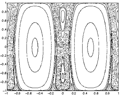
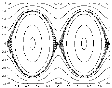
Figure 2: Phase space structure of the normalized equations (15) with $\bar{L}=2$, $\omega=\eta=F=1$, and $\Omega=\epsilon=0.1$. Left panel: $\gamma=0.8$. Right panel: $\gamma=2$. In both panels the horizontal and vertical axes indicate $\bar{g}/\pi$ and $\bar{G}/\bar{L}$, respectively.

For $\gamma\bar{L}\geq 2\eta\omega^{3}$, equation (22) represents a heteroclinic orbit which connects $S_{0}$ to $S_{2}$. For $\eta\omega^{3}<\gamma\bar{L}<2\eta\omega^{3}$, the heteroclinic orbit disappears and it is replaced by a homoclinic orbit (see Figure 1). To compute the explicit form of the homoclinic (or heteroclinic) orbit of (21), we use (21b) and (22), and obtain

$$\int^{\bar{G}_{\rm h}(\tau)}_{\bar{G}_{\rm h}(0)}\frac{{\rm d}\bar{G}}{\bar{G}\sqrt{1-\alpha\bar{G}^{2}}}=\pm\sqrt{\beta}\tau,$$ (23)

$$\alpha=\frac{\gamma^{2}}{16\eta\beta\omega^{4}},~{}~{}\beta=\frac{\gamma\bar{L}-\eta\omega^{3}}{4\omega},$$

where the lower integration limit is $\bar{G}_{\rm h}(0)=1/\sqrt{\alpha}$. After taking the integral (23), we arrive at

$$\bar{G}_{\rm h}(\tau) = \frac{\rm sech(\sqrt{\beta}\>\tau)}{\sqrt{\alpha}},$$ (24)

for the $\bar{G}\geq 0$ branch of the homoclinic (heteroclinic) orbit. Having $\bar{G}_{\rm h}(\tau)$, it is straightforward to calculate $\cos[2\bar{g}_{\rm h}(\tau)]$ and $\sin[2\bar{g}_{\rm h}(\tau)]$, and determine the explicit form of $\mathbf{q}_{\rm h}(\tau)=\left[\bar{g}_{\rm h}(\tau),\bar{G}_{\rm h}(\tau)\right]$.

For constructing $M_{2}(\tau_{0})$, we use Françoise’s FR96 ; PRK01 algorithm that has been devised for dynamical systems with polynomial nonlinearities. To express the averaged Hamiltonian $K$ in terms of polynomial functions of some new dependent variables, we utilize Hopf’s variables

$$Q_{1} = \frac{1}{2\omega}\sqrt{\bar{L}^{2}-\bar{G}^{2}}\cos(2\bar{g}),$$ (25a)

$$Q_{2} = \frac{1}{2\omega}\sqrt{\bar{L}^{2}-\bar{G}^{2}}\sin(2\bar{g}),$$ (25b)

and obtain the following differential 1-form for the evolution of the averaged system

$${\partial K_{1}\over\partial Q_{1}}{\rm d}Q_{1}+{\partial K_{1}\over\partial Q_{2}}{\rm d}Q_{2}$$ (26)

$$+ \epsilon\left[\left(s_{1}+\epsilon s_{2}\right){\rm d}Q_{2}-\left(z_{1}+\epsilon z_{2}\right){\rm d}Q_{1}\right]=0.$$

Here, the first-order Hamiltonian is

$$K_{1}(Q_{1},Q_{2})=\frac{\gamma}{2}(Q^{2}_{1}+Q^{2}_{2})-\frac{\eta\omega^{2}}{2}Q_{1}+C,$$ (27)

and

$$s_{1} = m_{1}Q_{2},$$ (28a)

$$z_{1} = n_{1}Q_{1}+n_{6},$$ (28b)

$$s_{2} = m_{2}(Q^{2}_{1}+Q^{2}_{2})Q_{2}+m_{3}Q_{1}Q_{2}+m_{4}Q_{2}$$ (28c)

$$+ m_{5}\sin(2\Omega\tau),$$

$$z_{2} = n_{2}(Q^{2}_{1}+Q^{2}_{2})Q_{1}+n_{3}(3Q^{2}_{1}+Q^{2}_{2})+n_{4}Q_{1}$$ (28d)

$$+ n_{5}\cos(2\Omega\tau)+n_{7}.$$

The constant coefficients $C$, $m_{i}$ ($i=1,\cdots,5$), and $n_{j}$ ($j=1,\cdots,7$) have been given in Appendix B. A prerequisite for the application of Françoise’s FR96 algorithm is that for all polynomial 1-forms $D$ that satisfy the condition

$$\int_{\textbf{q}_{\rm h}}D\equiv 0,$$ (29)

there must exist polynomials $A(Q_{1},Q_{2})$ and $r(Q_{1},Q_{2})$ such that $D={\rm d}A+r{\rm d}K_{1}$. We call this the condition $(*)$ and prove in Appendix C that $K_{1}$ satisfies the condition $(*)$.

Françoise’s algorithm states that if $M_{1}(\tau_{0})=\cdots=M_{k-1}(\tau_{0})\equiv 0$ for some integer $k\geq 2$, it follows that

$$M_{k}(\tau_{0}) = \int_{\textbf{q}_{\rm h}}D_{k},$$ (30a)

$$D_{1} = \delta_{1},\ D_{m}=\delta_{m}+\sum_{i+j=m}r_{i}\delta_{j},$$ (30b)

$$\delta_{j} = z_{j}{\rm d}Q_{1}-s_{j}{\rm d}Q_{2},$$ (30c)

for $2\leq m\leq k$. The functions $r_{i}$ are then determined successively from the formulas $D_{i}={\rm d}A_{i}+r_{i}{\rm d}K_{1}$ for $i=1,\cdots,k-1$. We have already found that

$$M_{1}(\tau_{0}) = \int_{\textbf{q}_{\rm h}}\delta_{1}=0,$$ (31)

$$\delta_{1} = (n_{1}Q_{1}+n_{6}){\rm d}Q_{1}-m_{1}Q_{2}{\rm d}Q_{2}.$$ (32)

From (30) and (46) it can be shown that

$$M_{2}(\tau_{0})=\int_{\textbf{q}_{\rm h}}\delta_{2}.$$ (33)

Substituting (30c) and (28) into (33), and carrying out the integration along $\textbf{q}_{\rm h}(\tau)$, result in

$$M_{2}(\tau_{0})=\frac{3\gamma F^{2}I}{2\omega^{6}}\sin(2\Omega\tau_{0}),$$ (34)

with $I$ being a constant (see Appendix D). Equation (34) shows that $\tau_{n}=n\pi/(2\Omega)$ ($n=1,2,\cdots$) are simple zeros of $M_{2}(\tau_{0})$ so that

$$M_{2}(\tau_{n})=0,~{}~{}\frac{\partial M_{2}(\tau_{0})}{\partial\tau_{0}}\Big{|}_{\tau_{0}=\tau_{n}}\neq 0.$$ (35)

Thus, we conclude that the global stable and unstable manifolds of the saddle point $S^{\tau_{0}}_{n}$, $W^{s}(S^{\tau_{0}}_{n})$ and $W^{u}(S^{\tau_{0}}_{n})$, always intersect transversely. Transversal intersections cause a sensitive dependence on initial conditions due to the Smale-Birkhoff homoclinic theorem. This is a route to chaos. On the other hand this means that the reduced equations (15) are non-integrable for $F\not=0$.

V Classification of circumferential waves

For $F=0$, h does not depend on $\tau$ and the normalized equations (15) are integrable. In such a circumstance, the phase space structure can take three general topologies (depending on the values of the system parameters and $\bar{L}$) as shown in Figure 1. In the first topology all stationary points with the coordinates $(\bar{g}_{s},\bar{G}_{s})$ calculated from

$$\textbf{f}(\bar{g}_{s},\bar{G}_{s})+\epsilon\textbf{h}(\bar{g}_{s},\bar{G}_{s},\epsilon)=\textbf{0},$$ (36)

are centers and they lie on the $\bar{G}=0$ axis with $\bar{g}_{s}=-\pi+n\pi/2$ ($n=0,\cdots,4$). In the second and third topologies, two off-axis centers (with $\bar{G}_{s}\not=0$) come to existence for $\bar{g}_{s}=\pm n\pi$ ($n=0,1$) and the on-axis stationary points with the same $\bar{g}_{s}=\pm n\pi$ become saddles. In the second topology, each saddle point is connected to itself by a homoclinic orbit, and in the third topology, a heteroclinic orbit connects two neighboring saddle points. The system with heteroclinic orbits allows for rotational $\bar{g}(\tau)$ while in the system with homoclinic orbits $\bar{g}(\tau)$ is always librating. Beware that this classification of phase space flows is valid as long as $\epsilon$ is sufficiently small.

For $F=0$, the phase space flows of (15) are structurally stable (with no unbounded branches) and the whole $(\bar{g},\bar{G})$-space is occupied by periodic orbits of period $T(K)$. At the stationary points, one has $T(K(\bar{g}_{s},\bar{G}_{s},\bar{L}))=0$. Given the invariance of $\bar{L}$, and the periodic solutions $\bar{g}(\tau)=\bar{g}(\tau+T(K))$ and $\bar{G}(\tau)=\bar{G}(\tau+T(K))$, the anomaly $\bar{l}$ is determined through solving

$${{\rm d}\bar{l}\over{\rm d}t}=\omega+\epsilon{\partial\over\partial\bar{L}}\left(K_{1}+{\epsilon\over 2!}K_{2}+{\epsilon^{2}\over 3!}K_{3}\right),$$ (37)

which results in $\bar{l}=\omega t+\epsilon R(\tau)$ with $R(\tau)=R(\tau+T(K))$. According to (9), the functions $g(t)$, $G(t)$ and $L(t)$ are also periodic in $t$ and we conclude that $l(t)=\omega t+R_{W}(t)$ with $R_{W}(t)=E_{W}(\bar{l})-\omega t$ being a small-amplitude periodic function of $t$. The explicit from of the circumferential wave will then become

$$\!\!\!{w(R,\phi,t)\over U_{m}(R)}=\sqrt{L(t)\!+\!G(t)\over 2\omega}\cos\left[n\phi\!-\!\omega t\!-\!R_{W}(t)\!-\!g(t)\right]$$

$$\!\!\qquad-\sqrt{L(t)\!-\!G(t)\over 2\omega}\cos\left[n\phi\!+\!\omega t\!+\!R_{W}(t)\!-\!g(t)\right],$$ (38)

which is composed of a forward and a backward traveling wave. Due to the periodic nature of $L(t)$ and $G(t)$, when the amplitude of the forward traveling wave is maximum, that of the backward wave is minimum and vice versa.

As our results of §IV shows, the regular nature of traveling waves is destroyed for $F\not=0$ and a chaotic layer occurs through the destruction of the homoclinic and heteroclinic orbits of (21). This happens over the time scale $\tau\sim{\cal O}(\epsilon^{-2})$ or $t\sim{\cal O}(\epsilon^{-3})$ (because $\bar{p}$ is present only in $K_{3}$). Figure 2 shows Poincaré maps of the system (15) for $F\not=0$. The sampling time step in generating the Poincaré maps has been $2\pi/\Omega$. It is seen that most tori around elliptic fixed points are preserved. They correspond to regular periodic and quasi-periodic solutions of the normalized system. For chaotic flows, the functions $\bar{g}(\tau)$ and $\bar{G}(\tau)$ randomly change within the invariant measure of the chaotic set. Consequently, the original Lissajous variables $g(t)$, $L(t)$, $G(t)$ and also $R_{W}(t)$ become chaotic too.

For $\bar{G}(\tau)>0$ and $\bar{G}(\tau)<0$ the forward and the backward traveling waves are the dominant components of the circumferential wave, respectively. When the chaotic layer emerges from the destroyed homoclinic orbits (left panel in Figure 2), the sign of $\bar{G}(\tau)$ is randomly switched along a chaotic trajectory. This means a random transfer of kinetic/potential energy between the forward and backward traveling wave components. For chaotic trajectories of this kind the angle $\bar{g}(\tau)$ randomly fluctuates near $\bar{g}\approx\pm n\pi$ ($n=0,1$) with an almost zero average. The evolution of circumferential waves is quite different when the chaotic layer emerges due to destroyed heteroclinic orbits (right panel in Figure 2). In this case chaos means a random change between the librational and rotational states of $\bar{g}(\tau)$. Such a change induces an unpredictable phase shift of magnitude $\pi$ for both forward and backward traveling wave components. We note that $\bar{G}(\tau)$ can flip sign on a chaotic trajectory only when $\bar{g}(\tau)$ is in its librational state.

VI concluding remarks

Resonance overlapping Ch79 ; Cont02 is the main cause for chaotic behavior in spinning disks with near-resonant angular velocities RM01 ; JA1 . The chaos predicted in this paper, however, happens far from fundamental resonances. Optical and HHDs are usually operated below critical resonant speeds and the lateral force $F$ due to magnetic head is very small. We showed that whatever the magnitude of $F$ may be, a chaotic layer fills some parts of the phase space because the Melnikov function of the normalized equations has always simple zeros. Dynamics of rotating disks is regular only if $F$ vanishes, which is an unrealistic assumption for disk drives. In low-speed disks with small $F$, diffusion of chaotic orbits (within their invariant measure) takes a long time of $t\sim{\cal O}(\epsilon^{-3})$. The slow development of chaotic circumferential waves makes them undetectable in short time scales at which most controllers work. The Melnikov function (34) depends not only on $F$, but also on the parameter $\eta$ through the constant $I$. The parameter $\eta$ is a contribution of imperfections, which are likely because of limited fabrication precision in micro/nano scales. For a perfect disk with $\eta=0$, the off-axis elliptic stationary points of (21), and consequently, homoclinic and heteroclinic orbits disappear. In such a condition the Melnikov function is indefinite, but the system admits an exact first integral and the dynamics is governed by the Hamiltonian function given in equation (11) of Jalali and Angoshtari JA1 .

One of the most important achievements of this work was to unveil the fact that it is premature to truncate the series of canonical perturbation theories before recording the role of all participating variables. In systems with non-autonomous governing ODEs (non-conservative systems), one must be cautious while removing a fast angle through averaging schemes. The removal of the fast angle may also wipe out time-dependent terms, up to some finite orders of $\epsilon$, and hide some essential information of the underlying dynamical process. Strange irregular solutions can indeed occur at any order and influence the long term response of dynamical systems as we observed for the spinning disk problem by keeping the third-order terms.

Appendix A The normalized Hamiltonian

By evaluating the integrals in (13), we obtain the first, second and third order terms of the normalized Hamiltonian as

$$K_{1} = \frac{-\gamma\bar{G}^{2}}{8\omega^{2}}+\frac{{\bar{L}}(3\gamma{\bar{L}}+2\eta\omega^{3})}{8\omega^{2}}+\Omega{\bar{P}}$$ (39)

$$- \frac{\eta\omega}{4}\sqrt{\bar{L}^{2}-\bar{G}^{2}}\cos(2\bar{g}),$$

$$K_{2} = -\frac{1}{64\omega^{5}}\Big{[}2\bar{L}(-9\bar{G}^{2}+17\bar{L}^{2})\gamma^{2}+64F^{2}\omega^{3}$$ (40)

$$+ 8(3\bar{L}^{2}-\bar{G}^{2})\gamma\eta\omega^{3}+8\bar{L}\eta^{2}\omega^{6}$$

$$+ 4\omega^{3}[-6\bar{L}\gamma\eta-2\eta^{2}\omega^{3}]\sqrt{\bar{L}^{2}-\bar{G}^{2}}\cos(2\bar{g})\Big{]},$$

$$K_{3} = \frac{3}{512\omega^{8}}\Big{\{}11\bar{G}^{4}\gamma^{3}-258\bar{G}^{2}\bar{L}^{2}\gamma^{3}+375{\bar{L}}^{4}\gamma^{3}$$ (41)

$$+ 1024F^{2}{\bar{L}}\gamma\omega^{3}-180{\bar{G}}^{2}{\bar{L}}\gamma^{2}\eta\omega^{3}+340{\bar{L}}^{3}\gamma^{2}\eta\omega^{3}$$

$$+ 256F^{2}\eta\omega^{6}-48{\bar{G}}^{2}\gamma\eta^{2}\omega^{6}+176{\bar{L}}^{2}\gamma\eta^{2}\omega^{6}$$

$$+ 32{\bar{L}}\eta^{3}\omega^{9}-2\omega^{3}\Big{[}17(10{\bar{L}}^{2}-{\bar{G}}^{2})\gamma^{2}\eta$$

$$+ 96{\bar{L}}\gamma\eta^{2}\omega^{3}+16\eta^{3}\omega^{6}\Big{]}\sqrt{{\bar{L}}^{2}-{\bar{G}}^{2}}\cos(2{\bar{g}})$$

$$- 16({\bar{G}}^{2}-{\bar{L}}^{2})\gamma\eta^{2}\omega^{6}\cos(4{\bar{g}})+256F^{2}\eta\omega^{6}\cos(2{\bar{p}})$$

$$- 512F^{2}\gamma\omega^{3}\sqrt{{\bar{L}}^{2}-{\bar{G}}^{2}}\cos(2{\bar{g}}-2{\bar{p}})\Big{\}}.$$

Consequently, the functions $d_{i}(\bar{L},\bar{G})$ in equations (III) are found to be

$$d_{1} = \frac{\eta\omega{\bar{G}}}{4}\left({\bar{L}}^{2}-{\bar{G}}^{2}\right)^{-1/2},$$

$$d_{2} = -\frac{{\bar{G}}}{16\omega^{2}}(6{\bar{L}}\gamma\eta+2\eta^{2}\omega^{3})({\bar{L}}^{2}-{\bar{G}}^{2})^{-1/2},$$

$$d_{3} = \frac{3{\bar{G}}}{256\omega^{5}}\Big{[}16\eta^{3}\omega^{6}+51(4{\bar{L}}^{2}-{\bar{G}}^{2})\gamma^{2}\eta$$

$$+ 96{\bar{L}}\gamma\eta^{2}\omega^{3}\Big{]}({\bar{L}}^{2}-{\bar{G}}^{2})^{-1/2},$$

$$d_{4} = -\frac{3{\bar{G}}\gamma\eta^{2}}{16\omega^{2}},$$

$$d_{5} = \frac{3{\bar{G}}F^{2}\gamma}{\omega^{5}}({\bar{L}}^{2}-{\bar{G}}^{2})^{-1/2},$$

$$d_{6} = -\frac{\gamma{\bar{G}}}{4\omega^{2}},$$

$$d_{7} = \frac{{\bar{G}}}{32\omega^{5}}(18{\bar{L}}\gamma^{2}+8\gamma\eta\omega^{3}),$$

$$d_{8} = \frac{3{\bar{G}}}{256\omega^{8}}\Big{[}2\gamma^{3}(11{\bar{G}}^{2}-129{\bar{L}}^{2})-180{\bar{L}}\gamma^{2}\eta\omega^{3}$$ (42)

$$- 48\gamma\eta^{2}\omega^{6}\Big{]}.$$

Defining $S=(\bar{L}^{2}-\bar{G}^{2})/{\bar{G}}$, the functions $e_{j}(\bar{L},\bar{G})$ in equations (III) become

$$e_{j} = -2d_{j}S,\ \ j=1,\ldots,5,\>j\neq 3,$$

$$e_{3} = -\frac{3}{128\omega^{5}}\Big{[}16\eta^{3}\omega^{6}+17(10{\bar{L}}^{2}-{\bar{G}}^{2})\gamma^{2}\eta$$ (43)

$$+ 96{\bar{L}}\gamma\eta^{2}\omega^{3}\Big{]}\sqrt{{\bar{L}}^{2}-{\bar{G}}^{2}}.$$

Appendix B

The constant coefficients of equations (27) and (28) are as follows

$$C = \frac{{\bar{L}}(\gamma{\bar{L}}+\eta\omega^{3})}{4\omega^{2}},$$

$$n_{1} = \frac{1}{8\omega^{3}}(9{\bar{L}}\gamma^{2}+4\gamma\eta\omega^{3}),$$

$$n_{2} = -\frac{33\gamma^{3}}{48\omega^{4}},$$

$$n_{3} = \frac{17\gamma^{2}\eta}{64\omega^{2}},$$

$$n_{4} = -\frac{1}{32\omega^{6}}(59{\bar{L}}^{2}\gamma^{3}+45{\bar{L}}\gamma^{2}\eta\omega^{3}+16\gamma\eta^{2}\omega^{6}),$$

$$n_{5} = \frac{F^{2}\gamma}{\omega^{4}},$$

$$n_{6} = -\frac{3{\bar{L}}\gamma\eta+\eta^{2}\omega^{3}}{8\omega},$$

$$n_{7} = \frac{1}{256\omega^{4}}(153{\bar{L}}^{2}\gamma^{2}\eta+96{\bar{L}}\gamma\eta^{2}\omega^{3}+16\eta^{3}\omega^{6}),$$

$$m_{i} = -n_{i},\ \ i=1,2,5,$$

$$m_{3} = -2n_{3},$$

$$m_{4} = \frac{1}{32\omega^{6}}(59{\bar{L}}^{2}\gamma^{3}+45{\bar{L}}\gamma^{2}\eta\omega^{3}+8\gamma\eta^{2}\omega^{6}).$$

Appendix C

In this appendix we prove that $K_{1}(Q_{1},Q_{2})$ given in (27), satisfies the condition $(*)$. To this end, we need the following theorem.

Theorem 1. Any polynomial 1-form $D$ of degree $n$ in $Q_{1}$ and $Q_{2}$ can be expressed as

$$D={\rm d}A+r{\rm d}K_{1}+\xi(K_{1})Q_{2}{\rm d}Q_{1},$$ (45)

where $A(Q_{1},Q_{2})$ and $r(Q_{1},Q_{2})$ are polynomials of degree $(n+1)$ and $(n-1)$ respectively, and $\xi(K_{1})$ is a polynomial of degree $[\frac{1}{2}(n-1)]$ where $[x]$ denotes the greatest integer in $x$.

Iliev IL99 has proved the same theorem for $H=(Q^{2}_{1}+Q^{2}_{2})/2$. Theorem 1 can thus be proved in a similar manner. Here we only present a useful result.

Let $D$ be a general polynomial 1-form of degree 1,

$$D=(a_{10}Q_{1}+a_{01}Q_{2}+a_{00}){\rm d}Q_{1}$$

$$+(b_{10}Q_{1}+b_{01}Q_{2}+b_{00}){\rm d}Q_{2},$$ (46a)

then in (45) we have

$$A(Q_{1},Q_{2}) = \frac{a_{10}}{2}Q^{2}_{1}+b_{10}Q_{1}Q_{2}+\frac{b_{01}}{2}Q^{2}_{2}$$ (46b)

$$+ a_{00}Q_{1}+b_{00}Q_{2},$$

$$r(Q_{1},Q_{2}) = 0,$$ (46c)

$$\xi(K_{1}) = a_{01}-b_{10}.$$ (46d)

Since ${\rm d}K_{1}=0$ along any phase space orbit characterized by $K_{1}(Q_{1},Q_{2})=k$, and since the integral of an exact differential ${\rm d}A$ around any closed curve is zero, from (45) we obtain

$$\int_{\textbf{q}_{\rm h}}D = \xi(k)\int_{\textbf{q}_{\rm h}}Q_{2}{\rm d}Q_{1}$$

$$= \xi(k)\int^{+\infty}_{-\infty}Q_{2}(\tau)\frac{{\rm d}Q_{1}}{{\rm d}\tau}{\rm d}\tau.$$

On the other hand, from (25a) we have

$$\frac{{\rm d}Q_{1}}{{\rm d}\tau}=E(\tau)-2Q_{2},$$

where $E(\tau)$ is an even function of $\tau$. Given the fact that $Q_{2}$ is an odd function of $\tau$, we conclude that

$$\int_{\textbf{q}_{\rm h}}D=-2\xi(k)\int^{+\infty}_{-\infty}Q^{2}_{2}{\rm d}\tau.$$

Consequently, if $\int_{\textbf{q}_{\rm h}}D\equiv 0$, it follows that $\xi(k)\equiv 0$ and therefore $D={\rm d}A+r{\rm d}K_{1}$, which completes the proof.

Appendix D

In equation (34), the constant coefficient $I$ is

$$I = -\frac{64\pi\sqrt{\eta}\Omega^{2}\omega^{2}}{\gamma}{\rm csch}\left(\frac{\pi\Omega}{\sqrt{\beta}}\right)$$

$$+ \frac{\pi\omega\sqrt{\eta}(3\gamma{\bar{L}}-4\eta\omega^{3})(\beta+4\Omega^{2})}{\gamma\beta}{\rm sech}\left(\frac{\pi\Omega}{\sqrt{\beta}}\right)$$

$$- \frac{\pi\omega{\bar{L}}\sqrt{\eta}(3\beta-4\Omega^{2})}{\beta}{\rm sech}\left(\frac{\pi\Omega}{\sqrt{\beta}}\right)$$

$$+ \frac{4\pi\eta^{3/2}\omega^{4}}{\gamma}{\rm sech}\left(\frac{\pi\Omega}{\sqrt{\beta}}\right).$$

References

- (1) A. Raman and C. D. Mote Jr., Int. J. Non-Linear Mech., 36, 261 (2001).
- (2) M. A. Jalali and A. Angoshtari, Int. J. Non-Linear Mech., 41 , 726 (2006).
- (3) J. N. Reddy, Applied Functional Analysis and Variational Methods in Engineering ( McGraw-Hill, New York, 1986).
- (4) A. Raman and C. D. Mote Jr., Int. J. Non-Linear Mech., 34, 139 (1999).
- (5) J. Nowinski, ASME J. Appl. Mech., 72 (1964).
- (6) N. Baddour and J. W. Zu, Appl. Math. Modeling, 25, 541 (2001).
- (7) A. Deprit, Celest. Mech. Dyn. Astron., 51, 201 (1991).
- (8) A. Deprit, Celest. Mech. Dyn. Astron., 1, 12 (1969).
- (9) A. Deprit and A. Elipe, Celest. Mech. Dyn. Astron., 51, 227 (1991).
- (10) V. K. Melnikov, Trans. Moscow Math., 12, 1 (1963).
- (11) B. V. Chirikov, Physics Reports, 52, 263 (1979).
- (12) J. Guckenheimer and P. Holmes, Nonlinear Oscillations, Dynamical Systems, and Bifurcations of Vector Fields (Springer, New York, 1983).
- (13) J. P. Françoise, Ergod. Theory Dynam. Syst., 16, 87 (1996).
- (14) L. Perko, Differential Equations and Dynamical Systems, 3rd edition (Springer, New York, 2001).
- (15) I. D. Iliev, Math. Proc. Cambridge Phil. Soc., 127, 317 (1999).
- (16) G. Contopoulos, Order and Chaos in Dynamical Astronomy (Springer, New York, 2002).