What can be learned studying the distribution of the biggest fragment ?

Abstract

In the canonical formalism of statistical physics, a signature of a first order phase transition for finite systems is the bimodal distribution of an order parameter. Previous thermodynamical studies of nuclear sources produced in heavy-ion collisions provide information which support the existence of a phase transition in those finite nuclear systems. Some results suggest that the observable $Z_{1}$ (charge of the biggest fragment) can be considered as a reliable order parameter of the transition. This talk will show how from peripheral collisions studied with the INDRA detector at GSI we can obtain this bimodal behaviour of $Z_{1}$. Getting rid of the entrance channel effects and under the constraint of an equiprobable distribution of excitation energy ($E^{*}$), we use the canonical description of a phase transition to link this bimodal behaviour with the residual convexity of the entropy. Theoretical (with and without phase transition) and experimental $Z_{1}-E^{*}$ correlations are compared. This comparison allows us to rule out the case without transition. Moreover that quantitative conparison provides us with information about the coexistence region in the $Z_{1}-E^{*}$ plane which is in good agreement with that obtained with the signal of abnormal fluctuations of configurational energy (microcanonical negative heat capacity).

1 Introduction

It is well known that a Liquid-Gas phase transition (PT) occurs in van der Waals fluids. The similarity between inter-molecular and nuclear interactions leads to a qualitatively similar equation of state which defines the spinodal and coexistence zones of the phase diagram. That is why we expect a “Liquid-Gas like” PT for nuclei. The order parameter is a scalar (one dimension) and is, in this case, the density of the system (more precisely the density difference between the ordered and disordered phase). The energy is also an order parameter because the PT has a latent heat.
When an homogeneous system enters the spinodal region of the phase diagram, its entropy exhibits a convex intruder along the order parameter(s) direction(s). The system becomes unstable and decomposes itself in two phases. For finite systems, due to surface energy effects, we expect a residual convexity for the system entropy after the transition leading directly to a bimodal distribution (accumulation of statistics for large and low values) of the order parameter. The challenge is to select an observable connected to the theoretical order parameter of the transition, and to explore sufficiently the phase diagram to populate the coexistence region and its neighbourhood. Quasi-projectile sources produced in (semi-)peripheral collisions cover a large range of dissipation and consequently permit this sufficient exploration.
Several theoretical [1, 2] and experimental works [3, 4, 5] show that the biggest fragment has a specific behaviour in the fragmentation process. In particular its size is correlated to the excitation energy ($E^{*}$) of the sources. We can reasonably explore whether the $Z_{1}$-$E^{*}$ experimental plane shows a bimodal pattern. Other experimental signals obtained with multifragmentation data can be correlated with the presence of a phase transition in hot nuclei. Indeed, abnormal fluctuations of configurational energy (AFCE) [6, 7] can be related to the negative heat capacity signal [8], and the fossil signal of spinodal decomposition [9] can illustrate the density fluctuations occurring when the nuclei pass through the spinodal zone [10]. These two signals are not direct ones and need some hypotheses and/or high statistics. In this work we will present the study of the bimodality signal which is expected to be more robust and direct. We will also show that its observation reinforces the conclusions extracted from the two previous signals.

The idea is to show experimentally that the biggest fragment charge, $Z_{1}$, can be a reliable observable to the order parameter of the PT. After an introduction of the canonical ensemble, we explain the procedure of renormalization which allows to get rid of entrance channel and data sorting effects. Then, comparing experimental and canonical (E,Z1) distributions, we will show that the observed signal of bimodality is related to the abnormal convexity of the entropy of the system. At the end, we propose a localisation of the coexistence zone deduced from a comparison between experimental data and the canonical description of a PT.

2 Canonical description of first-order phase transition.

Let us consider an observable E, known on average, free to fluctuate. The least biased distribution will be a Boltzmann-Gibbs distribution (def. 1) [11]. If this observable is an order parameter of the system we have to distinguish two cases: with and without phase transition.

$$\mathrm{P^{can}_{\beta}(E)=\frac{1}{Z^{can}_{\beta}}e\;^{\;S(E)-\beta E}\;with\;Z^{can}_{\beta}=\int dE\;e\;^{\;S(E)-\beta E}}$$ (1)

$$\mathrm{S\left(E\right)\sim S\left(E_{\beta}\right)+\left(E-E_{\beta}\right)\frac{d}{dE}\;S\big{|}_{E_{\beta}}+\frac{1}{2}\left(E-E_{\beta}\right)^{2}\frac{d^{2}}{dE^{2}}\;S\big{|}_{E_{\beta}}}\qquad$$ (2)

For a one phase system (PT is not present), the microcanonical entropy, S(E)=log W(E) where W(E) is the number of microstates associated to the value of E, is concave everywhere. We can perform on it a saddle point approximation (eq. 2) around the average value of $E$, $E_{\beta}$, meaning that the canonical distribution has a simple gaussian shape (eq. 3).

$$\mathrm{P^{(s.g.)}_{\beta}(E)=\frac{1}{\sqrt{2\pi\sigma_{E}^{2}}}\;exp\left(-\frac{1}{2\sigma_{E}^{2}}\left(E-E_{\beta}\right)^{2}\right)\;with\;\sigma^{2}_{E}=-\left(\frac{d^{2}}{dE^{2}}\;S\big{|}_{E_{\beta}}\right)^{-1}}\qquad$$ (3)

$$\mathrm{P^{(s.g.)}(E^{*},Z_{1})=\frac{1}{\sqrt{2\pi det\Sigma}}\>e^{\;-\frac{1}{2}\vec{x}\Sigma^{-1}\vec{x}},\;\vec{x}=\left(\begin{array}[]{ccc}E^{*}-E_{\beta}\\ Z_{1}-Z_{\beta}\end{array}\right),\;\Sigma=\left(\begin{array}[]{ccc}\sigma_{E}^{2}&\rho\;\sigma_{E}\sigma_{Z}\\ \rho\;\sigma_{E}\sigma_{Z}&\sigma_{Z}^{2}\end{array}\right)}$$ (8)

The parameters of this gaussian are directly linked to the characteristics of the entropy. In the same way we can define the minimum biased two dimensional distribution for the ($E^{*}$,Z1) observables leading to a 2D simple gaussian distribution [12] (def. 8). Parameters of this function gathered in the variance-covariance matrix are also deduced from the curvature matrix of the 2D microcanonical entropy [12, 13].

$$\mathrm{P^{(d.g.)}(E^{*},Z_{1})=N_{liq}\times P_{liq}^{(s.g.)}(E^{*},Z_{1})+N_{gaz}\times P_{gaz}^{(s.g.)}(E^{*},Z_{1})}$$ (9)

When a system passes through a phase transition and enters in the spinodal region, the homogeneous system has a convex intruder in its microcanonical entropy along the order parameter(s) direction(s) [14]. Instabilities occur and, due to the finite size of the system, the surface energy effects cause the non-additivity of the entropy leading at the end of the PT to a residual convex entropy for the two-phase system even at equilibrium. We cannot describe anymore the microcanonical entropy with a single saddle point approximation but we can introduce a double saddle point approximation. In this case the canonical distribution of the ($E^{*}$,Z1) observables can be described as the sum of two 2D simple gaussian distributions, one for each phase (def. 9) [12, 13].
In the canonical ensemble, the energy distribution $P^{can}_{\beta}(E^{*})$ as well as the two-dimensional distribution $P^{can}_{\beta}(E^{*},Z1)$ are conditioned by the number of available states $\exp{S}$ with a Boltzmann factor ponderation. The convex intruder in $S$ leads to a bimodality in the distribution [12]. Experimentally, this relation is not so clear: the weight of the different states has no reason to be exponential and the measured distribution $P^{exp}_{\beta}(E^{*})$ is modified by a factor $g_{exp}(E^{*})$ which is determined in a large part by entrance channel effects and data sorting : $P^{exp}(E^{*},Z_{1})=e^{S(E^{*},Z_{1})}g_{exp}(E^{*})$. The relative population of the different values of the $E^{*}$ distribution looses its thermostatistic meaning ($P^{exp}(E^{*})\propto g_{exp}(E^{*})P^{can}_{\beta}(E^{*})e^{\beta E^{*}}$). We cannot therefore directly compare experimental and canonical distributions and deduce entropy properties of the system.

$$\mathrm{P_{\omega}^{exp}(E^{*},Z_{1})=\omega(E)\times P^{exp}(E^{*},Z_{1})}$$ (10)

$$\mathrm{with\;\omega(E^{*})=\left(\int P^{(exp)}(E^{*},Z_{1})\;dZ_{1}\right)^{-1}}$$

2.1 Renormalization method.

In [12], a method was proposed to get rid of the experimental effects. Assuming that the experimental bias $g_{exp}(E^{*})$ affects the $Z_{1}$ distribution only through its correlation with the deposited energy $E^{*}$ (phase space dominance), a renormalization of the ($E^{*}$,$Z_{1}$) distribution under the constraint of an equiprobable distribution of $E^{*}$ (eq. 10) allows to be $E^{*}$-shape independent. If the system passes through a PT and the correlation between $E^{*}$ and $Z_{1}$ is not a one-to-one correspondence, it could reflect a residual convex intruder of the entropy.

2.2 Spurious bimodality

In principle one can ask whether the renormalization procedure given by eq. 10 can create spurious bimodality. This does not seem to be the case for different schematic models [12] but cannot be excluded a priori. Another ambiguity arises from the fact that a physical bimodality can be hidden by the renormalization procedure if the correlation between $Z_{1}$ and $E^{*}$ is too strong. Bimodality can be also difficult to spot if the energy interval is not wide enough. For these reasons in the following we will compare the two canonical cases (with and without transition) with the experimental distribution, to check the validity of the obtained signal.

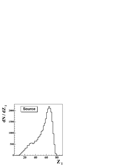
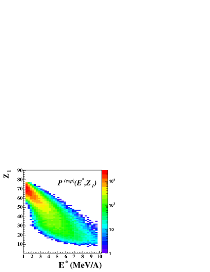
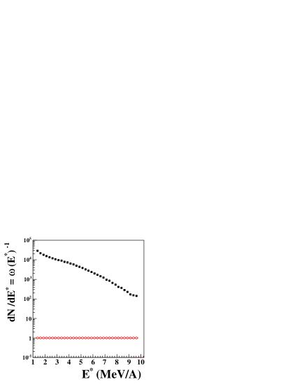
Figure 1: Upper part : left : experimental distribution of the argest size fragment ($Z_{1}$) of source events; right : experimental correlation between $Z_{1}$ and the excitation energy ($E^{*}$). Lower part : left : experimental reweighted correlation between $Z_{1}$ and the excitation energy; right : excitation energy ($E^{*}$) experimental distribution of source events in black squares; the open red circles show this distribution after the renormalization process. For this, we keep only $E^{*}$ bins with a statistics greater than 100.

3 Data selection and first observation of $Z_{1}$ distributions.

Data used in this present work are 80 MeV/A Au+Au reactions performed at the GSI facility and detected with the INDRA 4$\pi$ multidetector. We focus on peripheral and semi-peripheral collisions to study quasi-projectile sources (forward part of each event). To perform thermostatistical analyses, we select a set of events with a dynamically compact configuration for fragments, to reject dynamical events which are always present in heavy-ion reactions at intermediate energies. We require in addition a constant size of the sources to avoid size evolution effects in the bimodality signal [13, 15]. We evaluate the excitation energy using a standard calorimetry procedure [16, 17]. We compute the energy balance event-by-event in the centre of mass of the QP sources calculated with fragments only to minimize the effect of pre-equilibrium particles. Afterwards we keep only particles emitted in the forward part of the QP sources and double their contribution, assuming an isotropic emission. In figure 1 information on the experimental $Z_{1}$ and $E^{*}$ observables is shown, the latter covering a range between roughly 1 and 8 MeV/A (lower-right part). Spinodal zone limits obtained with the AFCE signal are around 2.5 and 5.8 MeV/A for this set of data [13]. The shape of the distribution $P^{exp}(E^{*},Z_{1})$ (upper right part) shows the dominance of low dissipation-large $Z_{1}$ events and reflects the cross-section distribution and data selection. If we look at the corresponding $Z_{1}$ distribution (upper left part) we do not see any clear signal of bimodality: a large part of statistics is around 65-70, and only a shoulder is visible around 30-40. This particular shape could reflect the lack of statistics for the ”gas-like” events. If we apply the renormalization procedure (eq. 10) we obtain (lower left part) a $P_{\omega}^{exp}(E,Z_{1})$ distribution which has a double humped shape, tending to prove that this procedure can reveal bimodality.

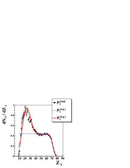
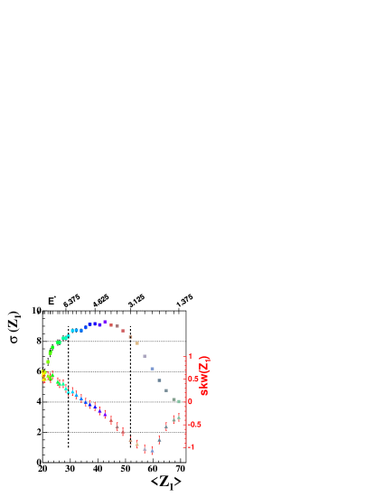
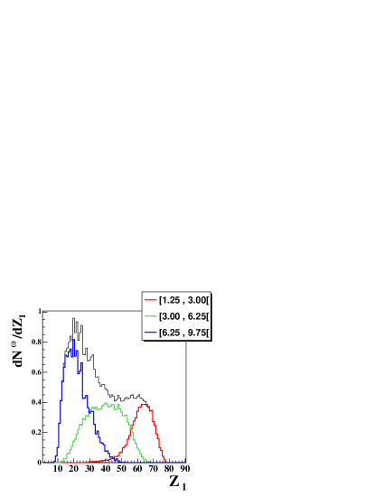
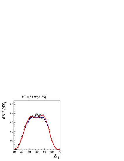
Figure 2: Upper part: left: Largest size fragment ($Z_{1}$) experimental reweighted distribution (black squares with error bars); the blue dashed curve corresponds to the best solution obtained by comparing data and a single gaussian function (concave entropy, no PT), the red continuous curve corresponds to the best solution obtained by comparing data and a double gaussian function (convex entropy, PT); right: microcanonical sampling (fixed $E^{*}$) of the mean, the RMS and the skewness of the $Z_{1}$ distributions. For each bin of $E^{*}$ (upper X axis), RMS (colored squares-left Y axis) and skewness (colored triangles-right Y axis) are plotted as a function of the mean value ($Z_{1}$-lower X axis); the two vertical dashed lines delimit the evaluated experimental spinodal zone where a quantitative comparison between data and PT case is performed. Lower part: left: same reweighted distribution of $Z_{1}$ as above (black curve); the three other distributions correspond to the three regions delimited by the vertical dashed lines (from left to right E$\in$[1.25,3.00[,[3.00,6.25[ and [6.25,9.75[); right: best solutions obtained after the 2D comparison between data and canonical PT case; results are plotted for the $Z_{1}$ axis projection; the two solutions correspond to two different ranges of $Z_{1}$ where fits have been performed Z1$\in$[25,55] (dashed curve) and Z1$\in$[10,79] (continuous curve). The corresponding parameter values are listed in table 1.

Parameters	[10,79]	[25,55]	Errors (%)
$\mathrm{\bar{E^{*}}_{liq}}$	2,10	1,67	23
$\mathrm{\sigma_{E^{*}_{liq}}}$	2,09	1,66	23
$\mathrm{\bar{Z_{1}}^{liq}}$	60,2	62,2	3
$\mathrm{\sigma_{Z_{1}^{liq}}}$	12,9	9,85	4
$\mathrm{\bar{E^{*}}_{gaz}}$	7,11	6,81	4
$\mathrm{\sigma_{E^{*}_{gaz}}}$	3,07	2,97	3
$\mathrm{\bar{Z_{1}}^{gaz}}$	21,1	23,8	12
$\mathrm{\sigma_{Z_{1}^{gaz}}}$	15,2	18,8	2
$\mathrm{\rho}$	-0,906	-0,860	4
$\mathrm{N_{liq}/N_{gaz}}$	1,12	0,66	52
$\mathrm{N_{dof}}$	605	387	-
$\mathrm{\chi^{2}}$	1488	646	-
$\mathrm{\chi^{2}/N_{dof}}$	2,459	1,669	-

Table 1: Parameters values for the two best reproductions of data by the double gaussian function $\mathrm{P^{(d.g.)}_{\omega}}$ for two ranges in $Z_{1}$ [10,79] (first column) et [25,55] (second column); the third column gives relative errors computed with the previous values; $\bar{E^{*}}$,$\bar{Z_{1}}$,$\sigma_{E^{*}}$,$\sigma_{Z_{1}}$ stand respectively for centroids and RMS in the two directions ($E,Z_{1}$) of each phase (liquid and gas). The $\rho$ parameter is the correlation factor ]-1,1[ between $Z_{1}$ and $E^{*}$ and the ratio $N_{liq}/N_{gaz}$ indicates the repartition of statistics between the two phases. The three last lines give the number of degrees of freedom and the absolute and normalized $\chi^{2}$ estimator values.

4 Canonical-Experimental comparisons.

To confirm that the two-hump distribution of $Z_{1}$ signals a convex intruder in the underlying entropy, in this section we compare the experimental reweighted distributions with the analytic expectation for a system exhibiting or not a first order PT. We apply the same renormalization to $P^{(s.g.)}_{\beta}(E)$ and $P^{(d.g.)}_{\beta}(E)$ and try to reproduce the data. We focus on the projection on the $Z_{1}$ axis to perform the fit. The results are shown in the upper left part of fig. 2. The scatter points with errors bars correspond to the data; the continuous (respectively dashed) curve corresponds to the best solution obtained for the double (respectively simple) reweighted gaussian. We can clearly distinguish the two behaviours, the no-transition case can not curve itself in the Z1=40-50 region and can only reproduce one phase. The fact that data are reproduced with the functional describing a first order transition allows us to associate the experimental bimodality signal to a genuine convexity of the system entropy. This confirms also that the $Z_{1}$ observable is linked to the order parameter of the transition. To obtain more quantitative information we have to better localize the spinodal region. To do this, we look at the second and third moments of the $Z_{1}$ distribution for each bin of $E^{*}$. Their evolution is plotted on the upper right part of fig. 2 as a function of the mean value of $Z_{1}$ (lower X axis) and $E^{*}$ (upper X axis). The squares (left Y axis) stand for the sigma ($\sigma$) of the distribution and the triangles (right Y axis) for the skewness (skw). $\sigma$ shows a maximum in the range 30-40 for $<Z_{1}>$. This maximum of fluctuations signs the core of the spinodal zone which corresponds to the hole in $P_{\omega}^{exp}(E,Z1)$ distribution. All values of $Z_{1}$, for a given $E^{*}$, are more or less equivalent. In the same region the skewness changes sign, illustrating the change in the distribution of asymmetry, with a value close to zero when the distribution approaches a normal one. The two vertical dashed lines on the plot delimit three regions (E$\in$[1.25,3.00[,[3.00,6.25[ and [6.25,9.75[) and the three corresponding $Z_{1}$ reweighted distributions are plotted in the lower left part of the same figure. The middle one, flat and broad, is very close to the behavior expected for a critical distribution [2] and illustrates the effect of an energy constraint on the order parameter distribution. If we had made a thinner range, we would have approached the microcanonical case. We select the region E$\in$[3.00,6.25[ to compare the two reweighted distributions $P_{\omega}^{exp}(E,Z_{1})$ and $P_{\omega}^{(d.g.)}(E,Z_{1})$ (eq. 9). The best solutions obtained after this 2D fit procedure are shown in the lower right part of figure 2 and table 1. They correspond to two ranges of $Z_{1}$ where fits are performed ([10,79] and [25,55]). These two best solutions are shown for the projection on the $Z_{1}$ axis.

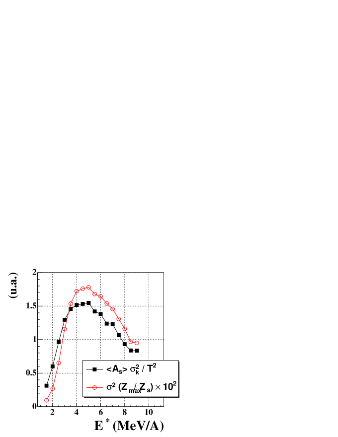
Figure 3: Microcanonical sample (fixed $E^{*}$) of the fluctuations of normalized FO kinetic energy (open circles) and largest fragment charge (full squares). T, As and Zs stand respectively for the temperature, the mass and charge of the source.

Using two different ranges for the $Z_{1}$ range allows us to estimate the sensitivity of the different parameters. The description of the two phases, given by a set of four parameters for each phase, can be summarized as follows: the average characteristics of the phases, given by $\bar{E^{*}}$, $\bar{Z_{1}}$, are well defined. The ratio between the populations of the liquid and gas phase strongly depends on the interval used to perform the fit. In the two cases the normalized estimator, $\chi^{2}$, is good. Concerning the $E^{*}$ axis, the values obtained for the liquid and gas phase centroids reflect the location of the coexistence zone, and are consistent with the location of the spinodal zone obtained with the AFCE signal with the same set of events [13, 18]. We can further explore the coherence between the two signals by looking at the fluctuations associated to $Z_{1}$ and to the Freeze-Out configurational kinetic energy [8]: we observe in fig. 3 that their evolution with excitation energy has a similar behaviour and exhibits a maximum for E$\sim$5MeV/A. This observation shows that we can consistently characterize the core of the spinodal zone with the maximum fluctuations of different observables connected to the order parameter of the phase transition.

5 Conclusion and outlook.

In this contribution we have shown that, taking into account the dynamics of the entrance channel and sorting effects with a renormalization procedure, the distribution of the largest size fragment ($Z_{1}$) of each event shows a bimodal pattern. The comparison with an analytical estimation assuming the presence (the absence) of a phase transition, shows that the experimental signal can be unambiguously associated to the case where the system has a residual convex intruder in its entropy. This link makes the $Z_{1}$ observable a reliable order parameter for the PT in hot nuclei. A bijective relation between the order of the transition and the bimodality signal has been proposed in [12] and analyses on data are in progress.

References

- [1] R. Botet et al., Phys. Rev. E 62 (2000) 1825.
- [2] F. Gulminelli et al., Phys. Rev. C 71 (2005) 054607.
- [3] J. D. Frankland et al. (INDRA and ALADIN collaborations), Phys. Rev. C 71 (2005) 034607.
- [4] J. D. Frankland et al. (INDRA and ALADIN collaborations), Nucl. Phys. A 749 (2005) 102.
- [5] M. Pichon et al. (INDRA and ALADIN collaborations), Nucl. Phys. A 279 (2006) 267.
- [6] N. Le Neindre, thèse de doctorat, Université de Caen (1999), http://tel.ccsd.cnrs.fr/tel-00003741.
- [7] M. D’Agostino et al., Phys. Lett. B 473 (2000) 219.
- [8] P. Chomaz et al., Nucl. Phys. A 647 (1999) 153.
- [9] G. Tăbăcaru et al., Eur. Phys. J. A 18 (2003) 103.
- [10] P. Chomaz et al., Phys. Rep. 389 (2004) 263 and references therein.
- [11] R. Balian, Cours de physique statistique de l’École Polytechnique, Ellipses (1983).
- [12] F. Gulminelli (2007), Nucl. Phys. A, in press.
- [13] E. Bonnet, thèse de doctorat, Université Paris-XI Orsay (2006), http://tel.ccsd.cnrs.fr/tel-00121736.
- [14] D. H. E. Gross, Microcanonical Thermodynamics-Phase Transitions in “Small” Systems, Singapore-World Scientific, 2001.
- [15] E. Bonnet et al. (INDRA and ALADIN collaborations) (2007) in preparation.
- [16] D. Cussol et al., Nucl. Phys. A 561 (1993) 298.
- [17] E. Vient et al. (INDRA Collaboration), Nucl. Phys. A 700 (2002) 555.
- [18] N. Le Neindre et al. (INDRA and ALADIN collaborations), Nucl. Phys. A (2007) submitted.