A Panchromatic Study of the Globular Cluster NGC 1904. I: The Blue Straggler Population 111Based on observations with the NASA/ESA HST, obtained at the Space Telescope Science Institute, which is operated by AURA, Inc., under NASA contract NAS5-26555. Also based on GALEX observations (program GI-056) and WFI observations collected at the European Southern Observatory, La Silla, Chile, within the observing programs 62.L-0354 and 64.L-0439.
Abstract
By combining high-resolution (HST-WFPC2) and wide-field ground based (2.2m ESO-WFI) and space (GALEX) observations, we have collected a multi-wavelength photometric data base (ranging from the far UV to the near infrared) of the galactic globular cluster NGC1904 (M79). The sample covers the entire cluster extension, from the very central regions up to the tidal radius. In the present paper such a data set is used to study the BSS population and its radial distribution. A total number of 39 bright () BSS has been detected, and they have been found to be highly segregated in the cluster core. No significant upturn in the BSS frequency has been observed in the outskirts of NGC 1904, in contrast to other clusters (M 3, 47 Tuc, NGC 6752, M 5) studied with the same technique. Such evidences, coupled with the large radius of avoidance estimated for NGC 1904 ( core radii), indicate that the vast majority of the cluster heavy stars (binaries) has already sunk to the core. Accordingly, extensive dynamical simulations suggest that BSS formed by mass transfer activity in primordial binaries evolving in isolation in the cluster outskirts represent only a negligible (0–10%) fraction of the overall population.
1 INTRODUCTION
Blue straggler stars (BSS) appear brighter and bluer than the Turn-Off (TO) point along an extension of the Main Sequence in color-magnitude diagrams (CMDs) of stellar populations. Hence, they mimic a young stellar population, with masses larger than the normal cluster stars (this is also confirmed by direct mass measurements; e.g. Shara, Saffer & Livio, 1997). BSS are thought to be objects that have increased their initial mass during their evolution, and two main scenarios have been proposed for their formation (e.g., Bailyn, 1995): the collisional scenario suggests that BSS are the end-products of stellar mergers induced by collisions (COL-BSS), while in the mass-transfer scenario BSS form by the mass-transfer activity between two companions in a binary system (MT-BSS), possibly up to the complete coalescence of the two stars (Mateo et al., 1990; Pritchet & Glaspey, 1991; Bailyn & Pinsonneault, 1995; Carney, Latham, & Laird, ; Tian et al., 2006; Leigh, Sills & Knigge, 2007). Hence, understanding the origin of BSS in stellar clusters provides valuable insight both on the binary evolution processes and on the effects of dynamical interactions on the (otherwise normal) stellar evolution. The MT formation scenario has by recently received further support by high-resolution spectroscopic observations, which detected anomalous Carbon and Oxygen abundances on the surface of a number of BSS in 47 Tuc (Ferraro et al., 2006a). However the role and relative importance of the two mechanisms are still largely unknown.
To clarify the BSS formation and evolution processes we studying the BSS radial distribution over the entire cluster extension in a number of galactic globular clusters (GCs). We completed such studies in 5 GCs: M 3 (Ferraro et al., 1997), 47 Tuc (Ferraro et al., 2004), NGC 6752 (Sabbi et al., 2004), Cen (Ferraro et al., 2006b), and M 5 (Lanzoni et al., 2007, see also Warren, Sandquist & Bolte 2006). Apart from Cen where mass segregation processes have not yet played a major role in altering the initial BSS distribution, the BSS are always highly concentrated in the cluster central regions. Moreover, in M 3, 47 Tuc, NGC 6752, and M 5 the BSS fraction decreases at intermediate radii and rises again in the outskirsts of the clusters, yielding a bimodal distribution. Preliminary evidences of such a bimodality have been found also in M 55 by Zaggia, Piotto & Capaccioli (1997). Recent dynamical simulations (Mapelli et al., 2004, 2006; Lanzoni et al., 2007) have been used to interpret the observed trends and have shown that a significant fraction (%) of COL-BSS is required to account for the observed BSS central peaks. In addition, a fraction of 20-40% MT-BSS is needed to reproduce the outer increase observed in these clusters. The case of Cen is reproduced by assuming that the BSS population in this cluster is composed entirely of MT-BSS. These results demonstrate that detailed studies of the BSS radial distribution within GCs are very powerful tools for better understanding the BSS formation channels and for probing the complex interplay between dynamics and stellar evolution in dense stellar systems.
In this paper we present multi-wavelength observations of NGC 1904. These observations are part of a coordinated project aimed at properly characterize the UV excess of old stellar aggregates as globular clusters, in terms of their hot stellar populations, like Horizontal Branch (HB) and Extreme HB stars, post-Asymptotic Giant Branch stars, BSS, etc. From integrated light measurements obtained with UIT (see Dorman, O’Connell & Rood, 1995), NGC 1904 was known to be relatively bright in the UV, and it was selected as a prime target in both our high-resolution (using HST) and wide-field (using GALEX) UV surveys. We have obtained a large set of data: (i) high-resolution ultraviolet (UV) and optical images of the cluster center have been secured with the WFPC2 on board HST; (ii) complementary wide-field observations covering the entire cluster extension have been obtained in the UV and optical bands by using the far- and near-UV detectors on board the Galaxy Evolution Explorer (GALEX) satellite and with ESO-WFI mounted at the 2.2 m ESO telescope, respectively. The combination of these datasets allowed a study of the structural properties of NGC 1904 (thus leading to an accurate redetermination of the center of gravity and the surface density profile), and of the radial distribution of the evolved stellar populations (in particular the BSS and horizontal branch star distributions have been derived over the entire cluster extension). While a companion paper (Schiavon et al. 2007, in preparation) will focus on the morphology and the structure of the HB, the present paper is devoted to the BSS population.
2 OBSERVATIONS AND DATA ANALYSIS
2.1 The data sets
The present study is based on a combination of different photometric data sets:
1. The high-resolution set – It consists of a series of UV, near UV and optical images of the cluster center obtained with HST-WFPC2 with two different pointings. In both cases the Planetary Camera (PC, the highest resolution instrument with ) has been pointed approximately on the cluster center to efficiently resolve the stars in the highly crowded central regions; the three Wide Field Cameras (WFC with resolution ) have been used to sample the surrounding regions. Observations in Pointing A (Prop. 6607, P.I. Ferraro) have been performed through filters F160BW (far-UV), F336W (approximately an filter) and F555W (), for a total exposure time , 4400, and 300 sec, respectively. Pointing B is a set of public HST-WFPC2 observations (Prop. 6095, P.I. Djorgovski) obtained through filters F218W (mid-UV), F439W () and F555W (). Because of the different orientations of the four cameras, this data set is complementary to the former (with the PC field of view in common), thus offering full coverage of the innermost regions of the cluster (see Figure 1). The combined photometric sample is ideal for efficiently studying both the hot stellar populations (as the BSS and the HB stars) and the cool red giant branch (RGB) population, and to guarantee a proper combination with the wide-field data set (see below).
The photometric reduction of both the high-resolution sets was carried out using ROMAFOT (Buonanno et al., 1983), a package developed to perform accurate photometry in crowded fields and specifically optimized to handle under-sampled Point Spread Functions (PSFs; Buonanno & Iannicola, 1989), as in the case of the HST-WFC chips. The standard procedure described in Ferraro et al. (1997, 2001) was adopted to derive the instrumental magnitudes and to calibrate them to the STMAG system by using the zero-points of Holtzman et al. (1995). The magnitude lists were finally cross-correlated in order to obtain a combined catalog.
2. The wide-field set - A complementary set of wide-field and images was secured by using the Wide Field Imager (WFI) at the 2.2m ESO-MPI telescope, during an observing run in January 1999 (Progr. ID: 062.L-0354, PI: Ferraro). A set of WFI images (Progr. ID: 064.L-0255) was also retrieved from the ESO-STECF Science Archive. Additional deep wide-field images were obtained in the UV band with the satellite GALEX (GI-056, P.I. Schiavon) through the FUV (1350–1750 Å) and NUV (1750–2800 Å) detectors. With a global field of view (FoV) of , the WFI observations cover the entire cluster extension. There is also full coverage of the cluster in the UV thanks to the large GALEX FoV, which is approximately in diameter and includes the WFI FoV (see Figure 2, where the cluster is roughly centered on WFI CCD ). However, because of the low resolution of the instrument ( and in the FUV and NUV channels, respectively), GALEX data have been used to sample only the external cluster regions not covered by HST.
The raw WFI images were corrected for bias and flat field, and the overscan regions were trimmed using IRAF222IRAF is distributed by the National Optical Astronomy Observatory, which is operated by the Association of Universities for Research in Astronomy, Inc., under cooperative agreement with the National Science Foundation. tools (mscred package). Standard crowded field photometry, including PSF modeling, was carried out independently on each image using DAOPHOTII/ALLSTAR (Stetson, 1987). For each WFI chip a catalog listing the instrumental and magnitudes was obtained by cross-correlating the single-band catalogs. Several hundred stars in common with Kravtsov et al. (1997), Stetson (2000), and Ferraro et al. (1992) have been used to transform the instrumental , , , and magnitudes to the Johnson/Cousins photometric system.
As for the WFI data, also for GALEX observations standard photometry and PSF fitting were performed independently on each image using DAOPHOTII/ALLSTAR. A combined FUV-NUV catalog was then obtained by cross-correlating the single-band catalogs.
2.2 Astrometry and homogenization of the catalogs
The HST, WFI, and GALEX catalogs have been placed on the absolute astrometric system by adopting the procedure already described in Ferraro et al. (2001, 2003). The new astrometric Guide Star Catalog (GSC-II333Available at http://www-gsss.stsci.edu/Catalogs/GSC/GSC2/GSC2.htm.) was used to search for astrometric standard stars in the WFI FoV, and a cross-correlation tool specifically developed at the Bologna Observatory (Montegriffo et al. 2003, private communication) has been employed to obtain an astrometric solution for each WFI chip. Several hundred GSC-II reference stars were found in each chip, thus allowing an accurate absolute positioning of the stars. Then, we used more than 3000 and 1500 bright WFI stars in common with the HST and GALEX samples, respectively, as secondary astrometric standards, so as to place all the catalogs on the same absolute astrometric system. We estimate that the global uncertainties in the astrometric solution is of the order of , both in right ascension () and declination ().
Once placed on the same coordinate system, the catalogs have been cross-correlated and the stars in common have been used to transform all the magnitudes in the same photometric system. In particular, the HST STMAG magnitudes have been converted to the WFI ones by using the stars in common between the two samples in the optical bands. Then, the GALEX FUV and NUV instrumental magnitudes have been calibrated onto the HST and magnitudes, respectively using the stars in common between the GALEX and HST samples.
At the end of the procedure a homogeneous master catalog of magnitudes and absolute coordinates of all the stars included in the HST, WFI, and GALEX samples was finally produced.
2.3 Center of gravity and definition of the samples
Once the absolute positions of individual stars have been obtained, the center of gravity of NGC 1904 has been determined by averaging the coordinates and of all stars lying in the PC FoV, following the iterative procedure described in Montegriffo et al. (1995, see also Ferraro et al. 2003, 2004). In order to correct for spurious effects due to incompleteness in the very inner regions of the cluster, we considered two samples with different limiting magnitudes ( and ), and we computed the barycenter of stars for each sample. The two estimates agree within , setting at , . The newly determined center of gravity is located at south-est (, ) from that previously derived by Harris (1996) on the basis of the surface brightness distribution.
In order to reduce spurious effects in the most crowded regions of the cluster due to the low resolution of the WFI and GALEX observations, we considered only the HST data for the inner from the center, this value being imposed by the geometry of the combined WFPC2 FoVs (see Figure 1). Thus, in the following we define as HST sample the ensemble of all the stars observed with HST at from , and as External sample all the stars detected with WFI and/or GALEX at , out to (see Figure 2). The CMDs of the HST and External samples in the planes are shown in Figure 3.
Note that only the data suitable for the study of the BSS population will be considered in the following, while those obtained through filters F160BW and FUV on board HST and GALEX, respectively, will be used in a forthcoming paper specifically devoted to the analysis the HB properties (Schiavon et al. 2007).
2.4 Density profile
Considering all the stars brighter than in the combined HST+External catalog (see Figure 3), we have determined the projected density profile of NGC 1904 by direct star counts over the entire cluster extension. Following the procedure already described in Ferraro et al. (1999a, 2004), we have divided the entire sample in 31 concentric annuli, each centered on and split in an adequate number of sub-sectors (quadrants for the annuli totally sampled by the observations, octants elsewhere). The number of stars lying within each sub-sector was counted, and the star density was obtained by dividing these values by the corresponding sub-sector areas. The stellar density in each annulus was then obtained as the average of the sub-sector densities, and the standard deviation was estimated from the variance among the sub-sectors.
The radial density profile thus derived is plotted in Figure 4, and the average of the three outermost () surface density measures has been adopted as the background contribution (corresponding to arcmin-2). Figure 4 also shows the mono-mass King model that best fits the derived density profile, with the corresponding values of the core radius and concentration being (with a typical error of ) and , respectively (hence, the tidal radius is ). These values are in good agreement with those quoted by Harris (1996, and ), Trager, Djorgovski & King (1993, and ), and McLaughlin & van der Marel (2005, and ), derived from the surface brightness profile, and they confirm that NGC 1904 has not yet experienced core collapse. By assuming a distance modulus (distance kpc, Ferraro et al., 1999b), the derived value of corresponds to pc. By summing the luminosities of stars with observed within , we estimate that the extinction-corrected central surface brightness of the cluster is mag/arcsec2, in good agreement with Harris (1996, ), Djorgovski (1993, ), and McLaughlin & van der Marel (2005, ). Following the procedure described in Djorgovski (1993, see also Beccari et al. 2006), we derive , where is the central luminosity density in units of Lpc3 (for comparison, in Harris, 1996; Djorgovski, 1993; McLaughlin & van der Marel, 2005).
3 THE BSS POPULATION OF NGC 1904
3.1 BSS selection
At UV wavelengths BSS are among the brightest objects in a GC, and RGB stars are particularly faint. By combining these advantages with the high-resolution capability of HST, the usual problems associated with photometric blends and crowding in the high density central regions of GCs are minimized, and BSS can be most reliably recognized and separated from the other populations in the UV CMDs. For these reasons our primary criterion for the definition of the BSS sample is based on the position of stars in the () plane (see also Ferraro et al., 2004, for a detailed discussion of this issue). In order to avoid incompleteness bias and the possible contamination from TO and sub-giant branch stars, we have adopted a limiting magnitude , roughly corresponding to 1 magnitude brighter than the cluster TO. The resulting BSS selection box in the UV CMD is shown in Figure 5. Once selected in the UV CMD, all the BSS lying in the field in common with the optical-HST sample have been used to define the selection box in the () and () planes. The limiting magnitude in the band is , and the adopted BSS selection boxes in these planes are shown in Figures 3 and 6 (only stars not observed in HST-Pointing B are shown in the latter).
With these criteria we have identified 39 BSS in NGC 1904: 37 in the HST sample (32 from HST-Pointing B, and 5 from HST-Pointing A) and 2 in the External sample (), the most distant lying at () from the cluster center (see Figure 2). All candidate BSS have been confirmed by visual inspection, evaluating the quality and the precision of the PSF fitting. This procedure significantly reduces the possibility of introducing spurious objects, such as blends, background galaxies, etc., in the sample. The coordinates and magnitudes of all the identified BSS are listed in Table 1.
In order to study the radial distribution of BSSs, one needs to compare their number counts as a function of radius with those of a population assumed to trace the radial density distribution of normal cluster stars. We chose to use HB stars for that purpose, given their high luminosities and relatively large number. Thanks to the (essentially blue) HB morphology, such a population can be easily selected in all CMDs, and the adopted selection boxes, designed to include the bulk of HB and the few post-HB stars, are shown in Figures 5–6. In order to be conservative, a few stars lying within the adopted HB selection boxes in the optical bands, but not detected in the UV filters (GALEX-NUV channel and HST-F218W filter), have been excluded from the following analysis. However slightly different boxes or the inclusion of these stars in the sample have no effects on the results. With these criteria we have identified 249 HB stars (197 at from the HST sample, and 52 at from the External sample).
3.2 BSS mass distribution
The position of BSS in the CMD can be used to derive a ”photometric ” estimate of their masses through the comparison with theoretical isochrones. We did this in the plane, where 34 BSS (32 from the HST-Pointing B and 2 from the External sample) out of the 39 identified in the cluster have been measured.
A set of isochrones of appropriate metallicity () has been extracted from the data-base of Cariulo, Degl’Innocenti & Castellani (2003) and transformed into the observational plane by adopting a reddening (Ferraro et al., 1999b). The 12 Gyr isochrone nicely reproduces the main cluster population, while the region of the CMD populated by the BSS is well spanned by a set of isochrones with ages ranging from 1 to 6 Gyr (see Figure 7). Thus, the entire dataset of isochrones available in this age range (stepped at 0.5 Gyr) has been used to derive a grid linking the BSS colors and magnitudes to their masses. Each BSS has been projected on the closest isochrone and a value of its mass has been derived. As shown in the lower panel of Figure 7, BSS masses range from to , and both the mean and the median of distribution correspond to 1.2 . The TO mass turns out to be .
3.3 The BSS radial distribution
The radial distribution of BSS identified in NGC 1904 has been studied following the same procedure previously adopted for other clusters (see references in Ferraro, 2006; Beccari et al., 2006). In Figure 8 we compare the BSS cumulative radial distribution to that of HB stars. The two distributions are obviously different, with the BSS being more centrally concentrated than HB stars. A Kolmogorov-Smirnov test gives a probability that they are extracted from the same population, i.e. the two populations are different at more than level.
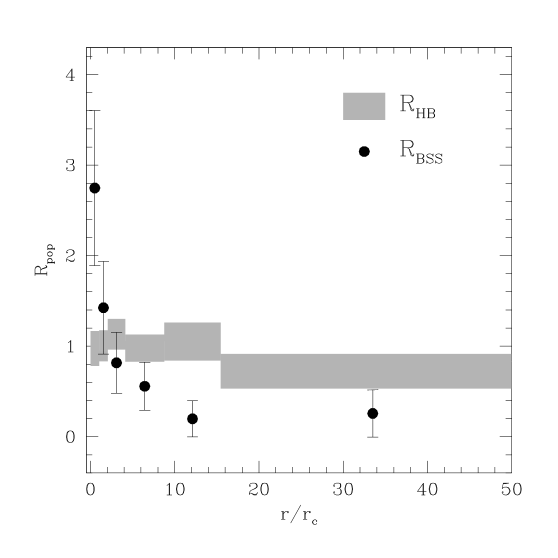
For a more quantitative analysis, the surveyed area has been divided into 6 concentric annuli, the first roughly corresponding to the core radius (), and the others chosen in order to sample approximately the same fraction of the cluster luminosity out to the tidal radius (). The luminosity in each annulus has been calculated by integrating the surface density profile shown in Figure 4. The number of BSS and HB stars ( and , respectively), as well as the fraction of sampled luminosity () measured in each annulus are listed in Table 2 and have been used to compute the population ratio and the specific frequencies (see Ferraro et al., 2003):
| (1) |
with pop = BSS, HB.
The resulting radial trend of over the surveyed area is essentially constant, with a value close to unity (see Figure 9). This is just what expected on the basis of the stellar evolution theory, which predicts that the fraction of stars in any post-main sequence evolutionary stage is strictly proportional to the fraction of the sampled luminosity (Renzini & Fusi Pecci, 1988). In contrast the BSS show a completely different radial distribution: as shown in Figure 9, the specific frequency is highly peaked at the cluster center decreases to a minimum at and remains approximately constant outwards. The same behavior is clearly visible also in Figure 10, where the population ratio is plotted as a function of .
3.4 Dynamical simulations
Following the same approach as Mapelli et al. (2004, 2006) and Lanzoni et al. (2007), we have used a Monte-Carlo simulation code (originally developed by Sigurdsson & Phinney, 1995) in order to reproduce the observed radial distribution and to derive some clues about the BSS formation mechanisms. Such a code follows the dynamical evolution of BSS within a background cluster, taking into account the effects of both dynamical friction and distant encounters. Since stellar collisions are most probable in the central high-density regions of the clusters, in the simulations we define COL-BSS those objects with initial positions . Since primordial binaries most likely evolve in isolation if they orbit in the cluster outskirts, we identify as MT-BSS those BSS having . Within these defintions, in any given run we assume that a certain fraction of the simulated BSS is made of COL-BSS and the remaining fraction of MT-BSS. The initial positions of the two types of BSS are randomly generated within the appropriate radial range ( for COL-BSS, and for the others) following a flat distribution, according to the fact that the number of stars in a King model scales as . Their initial velocities are randomly extracted from the cluster velocity distribution illustrated in Sigurdsson & Phinney (1995), and an additional natal kick is assigned to COL-BSS to account for the recoil induced by the three-body encounters that trigger the merger and produce the BSS (see, e.g., Sigurdsson, Davies & Bolte, 1994; Davies, Benz & Hills, 1994). Each BSS has characteristic mass and maximum lifetime . We follow their dynamical evolution in the (fixed) gravitational potential for a time (), where each is a randomly chosen fraction of . At the end of the simulation we register the final positions of BSS, and we compare their radial distribution with the observed one. The percentage of COL- and MT-BSS is changed and the procedure repeated until a reasonable agreement between the simulated and the observed distributions is reached.
For a more detailed discussion of the procedure and the ranges of values appropriate for the input parameters we refer to Mapelli et al. (2006). Here we only list the assumptions made in the present study:
-
–
the background cluster has been approximated with a multi-mass King model, determined as the best fit to the observed profile444By adopting the same mass groups as those of Mapelli et al. (2006), the resulting value of the King dimensionless central potential is . The cluster central velocity dispersion is set to (Dubath, Meylan & Mayor, 1997), and, assuming as the average mass of the cluster stars, the central stellar density is (Pryor & Meylan, 1993);
-
–
BSS masses have been fixed to (see Section 3.2) and characteristic lifetimes ranging between 1.5 and 4 Gyr have been considered;
-
–
COL-BSS have been distributed with initial positions and have been given a natal kick velocity of ;
-
–
initial positions ranging between and have been considered for MT-BSS in different runs;
-
–
in each simulation we have followed the evolution of BSS.
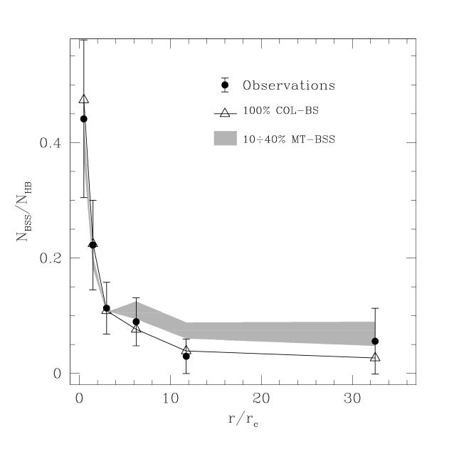
The simulated radial distribution that best reproduces the observed one (with a reduced ) is shown in Figure 10 and is obtained by assuming that the totality of BSS is made of COL-BSS. In the best-fit case the BSS characteristic lifetime is Gyr, but a variation between 1 and 4 Gyr of this parameter still leads to a very good agreement (–0.3) with the observations. For the sake of comparison, in Figure 10 we also show the results of the simulations obtained by assuming a percentage of MT-BSS ranging from 10% to 40% (see lower and upper boundaries of the gray region, respectively)555Note that a population of 40% MT-BSS was needed in order to reproduce the bimodal distribution observed in M 3, 47 Tuc and NGC 6752 (Mapelli et al., 2006), and 10% was found to be the appropriate percentage of MT-BSS in the case of M 5 (Lanzoni et al., 2007).. As can be seen, while a population of 10% MT-BSS is still marginally consistent with the observations, larger percentages systematically overestimate the BSS population at . Increasing the BSS mass up to does not change this conclusion.
By assuming 12 Gyr for the age of NGC 1904, we have used the simulations and the dynamical friction timescale (from, e.g., Mapelli et al., 2006) for stars to estimate the radius of avoidance of the cluster, i.e., the radius within which all these stars are expected to have already sunk to the cluster core because of mass segregation processes. We find that (i.e., ), which corresponds to a significant fraction of the entire cluster extension. This evidence is consistent with the fact that the simulated MT-BSS appear to be a negligible fraction of the overall BSS population.
4 DISCUSSION
We have studied the brightest portion () of the BSS population in NGC 1904. We have found a total of 39 objects, with a high degree of segregation in the cluster center. Approximately 38% of the entire BSS population is found within the cluster core, while only of HB stars are counted in the same region. This indicates a significant overabundance of BSS in the center, as also confirmed by the fact that the BSS specific frequency within is roughly 3 times larger than expected for a normal (non-segregated) population on the basis of the sampled light (see Figure 9). The peak value is in good agreement with what is found in the case of M 3, 47 Tuc, NGC 6752 and M 5 (see Ferraro et al., 2004; Sabbi et al., 2004; Lanzoni et al., 2007). Unlike these clusters, no significant upturn of the distribution at large radii has been detected in NGC 1904.
We emphasize that the absence of an external upturn in the BSS radial distribution is not an effect of low statistics. In the case of NGC 6752, where a similar amount of BSS (34) has been detected, the BSS radial distribution is clearly bimodal (Sabbi et al., 2004). This can be seen also in Figure 11, where the two distributions are directly compared. They nicely agree within , but the fraction of BSS in NGC 6752 rises again at larger distances from the center, despite the smaller number of BSS observed in this cluster compared to NGC 1904.
Extensive dynamical simulations have been used to derive some hints about the BSS formation mechanisms. Even if admittedly crude, this approach has been successfully used to demonstrate that the external rising branch of the BSS radial distribution observed in M 3, 47 Tuc, NGC 6752 and M 5 cannot be due to COL-BSS originated in the core and then kicked out in the outer regions: hence, a significant fraction (20-40%) of the overall population is required to be made of MT-BSS in these clusters (Mapelli et al., 2006; Lanzoni et al., 2007). By using the same simulations to interpret the (flat) BSS radial distribution of NGC 1904, we found that only a negligible percentage (0–10%) of MT-BSS is needed. However, we emphasize that if a rising peripheral BSS frequency is absent (as in the case of NGC 1904) our simple approach cannot distinguish between BSS created by MT (and then segregated into the cluster core by the dynamical friction) and COL-BSS created by collisions inside the core.
On the other hand, the negligible fraction of peripheral MT-BSS found in NGC 1904 is in agreement with the quite large value of the radius of avoidance estimated for this cluster (), which indicates that all the heavy stars (binaries) within this radial distance have had enough time to sink to the core and are therefore not expected in the cluster outskirts. Such a radial distance corresponds to , i.e., it represents a significant fraction of the cluster extension (only 1% of the cluster light is contained between and ), and hence only a small fraction of the massive objects are expected to be unaffected by the dynamical friction). In all the other studied cases, is significantly smaller: (Mapelli et al., 2006; Lanzoni et al., 2007). In turn, this suggests that at least a fraction of the BSS population that we now observe in the cluster center are primordial binaries which have sunk to the core because of the dynamical friction process, and mixed with those that formed through stellar collisions.
Only systematic surveys of physical and chemical properties for a large number of BSS in different environments (see examples in De Marco et al., 2005; Ferraro et al., 2006a) can definitively identify the formation processes of these stars.
References
- Bailyn & Pinsonneault (1995) Bailyn, C. D., & Pinsonneault, M. H. 1995, ApJ, 439, 705
- Bailyn (1995) Bailyn, C. D. 1995, ARA&A, 33, 133
- Beccari et al. (2006) Beccari, G., Ferraro, F. R., Lanzoni, B., & Bellazzini, M. 2006, ApJ, 652, L121
- Buonanno et al. (1983) Buonanno, R., Buscema, G., Corsi, C. E., Ferraro, I., & Iannicola, G. 1983, A&A, 126, 278
- Buonanno & Iannicola (1989) Buonanno, R., Iannicola, G. 1989, PASP, 101, 294
- Cariulo, Degl’Innocenti & Castellani (2003) Cariulo, P., Degl’Innocenti, S. & Castellani, V.,2003, A&A, 412, 1121
- (7) Carney, B. W., Latham, D. W., & Laird, J. B., 2005, AJ, 129, 466
- Davies, Benz & Hills (1994) Davies, M. B., Benz, W., & Hills, J. G. 1994, ApJ, 424, 870
- De Marco et al. (2005) De Marco, O., Shara, M. M., Zurek, D., Ouellette, J. A., Lanz, T., Saffer, R. A., & Sepinsky, J.F. 2005, ApJ, 632, 894
- Djorgovski (1993) Djorgovski, S. 1993, ASPC, 50, 373
- Dorman, O’Connell & Rood (1995) Dorman, B., O’Connell, R. W., & Rood, R. T. 1995, ApJ442, 105
- Dubath, Meylan & Mayor (1997) Dubath P., Meylan G., & Mayor M., 1997, A&A, 324, 505
- Ferraro et al. (1992) Ferraro, F. R., Clementini, G., Fusi Pecci, F., Sortino, R., Buonanno, R. 1992, MNRAS256, 391
- Ferraro et al. (1997) Ferraro, F. R., Paltrinieri, B., Fusi Pecci, F., Cacciari, C., Dorman, B., Rood, R. T., Buonanno, R., Corsi, C. E., Burgarella, D., & Laget, M., 1997, A&A, 324, 915
- Ferraro et al. (1999a) Ferraro, F. R., Paltrinieri, B., Rood, R. T., Dorman, B. 1999a, ApJ 522, 983
- Ferraro et al. (1999b) Ferraro F. R., Messineo M., Fusi Pecci F., De Palo M. A., Straniero O., Chieffi A., Limongi M. 1999b, AJ, 118, 1738
- Ferraro et al. (2001) Ferraro, F. R., D’Amico, N., Possenti, A., Mignani, R. P., & Paltrinieri, B. 2001, ApJ, 561, 337
- Ferraro et al. (2003) Ferraro, F. R., Sills, A., Rood, R. T., Paltrinieri, B., & Buonanno, R. 2003, ApJ, 588, 464
- Ferraro et al. (2004) Ferraro, F. R., Beccari, G., Rood, R. T., Bellazzini, M., Sills, A., & Sabbi, E. 2004, ApJ, 603, 127
- Ferraro (2006) Ferraro, F. R., 2006, in Resolved Stellar Populations, ASP Conference Series, 2005, D. Valls-Gabaud & M. Chaves Eds., astro-ph/0601217
- Ferraro et al. (2006a) Ferraro, F. R., et al. 2006a, ApJ, 647, L53
- Ferraro et al. (2006b) Ferraro, F. R., Sollima, A., Rood, R. T., Origlia, L., Pancino, E., & Bellazzini, M. 2006b, ApJ, 638, 433
- Harris (1996) Harris, W.E. 1996, AJ, 112, 1487
- Holtzman et al. (1995) Holtzman, J. A., Burrows, C. J., Casertano, S., Hester, J. J., Trauger, J. T., Watson, A. M., & Worthey, G. 1995, PASP, 107, 1065
- Kravtsov et al. (1997) Kravtsov, V., Ipatov, A., Samus, N., Smirnov, O., Alcaino, G., Liller, W., Alvarado, F. 1997, A&A, 125, 1
- Lanzoni et al. (2007) Lanzoni, B., Dalessandro, E., Ferraro, F. R., Mancini, C., Beccari, G., Rood, R. T., Mapelli, M., Sigurdsson, S. 2007, ApJin press (astro-ph/07040139)
- Leigh, Sills & Knigge (2007) Leigh, N., Sills, A., Knigge, C. 2007, ApJ in press (astro-ph/0702349)
- Mapelli et al. (2004) Mapelli, M., Sigurdsson, S., Colpi, M., Ferraro, F. R., Possenti, A., Rood, R. T., Sills, A., & Beccari, G. 2004, ApJ, 605, L29
- Mapelli et al. (2006) Mapelli, M., Sigurdsson, S., Ferraro, F. R., Colpi, M., Possenti, A., & Lanzoni, B. 2006, MNRAS, 373, 361
- Mateo et al. (1990) Mateo, M., Harris, H. C., Nemec, J., Olszewski, E. W., 1990, AJ, 100, 469
- McLaughlin & van der Marel (2005) McLaughlin, D. E., & van der Marel, R. P. 2005, ApJS, 161, 304
- Montegriffo et al. (1995) Montegriffo, P., Ferraro, F. R., Fusi Pecci, F., & Origlia, L. 1995, MNRAS, 276, 739
- Pritchet & Glaspey (1991) Pritchet, C. J., & Glaspey, J. W. 1991, ApJ, 373, 105
- Pryor & Meylan (1993) Pryor C., & Meylan G., 1993, Structure and Dynamics of Globular Clusters. Proceedings of a Workshop held in Berkeley, California, July 15-17, 1992, to Honor the 65th Birthday of Ivan King. Editors, S.G. Djorgovski and G. Meylan; Publisher, Astronomical Society of the Pacific, Vol. 50, 357
- Renzini & Fusi Pecci (1988) Renzini, A., & Fusi Pecci, F. 1988, ARA&A, 26, 199
- Sabbi et al. (2004) Sabbi, E., Ferraro, F. R., Sills, A., Rood, R. T., 2004, ApJ 617, 1296
- Shara, Saffer & Livio (1997) Shara, M. M., Saffer, R. A., & Livio, M. 1997, ApJ, 489, L59
- Sigurdsson, Davies & Bolte (1994) Sigurdsson, S., Davies, M. B., & Bolte, M. 1994, ApJ, 431, L115
- Sigurdsson & Phinney (1995) Sigurdsson S., Phinney, E. S., 1995, ApJS, 99, 609
- Stetson (1987) Stetson, P. B. 1987, PASP, 99, 191
- Stetson (2000) Stetson, P. B. 2000, PASP, 112, 925, (for the photometric standards list see http://cadcwww.hia.nrc.ca/standards/ )
- Tian et al. (2006) Tian, B., Deng, L., Han, Z., Zhang, X. B. 2006, A&A 455, 247
- Trager, Djorgovski & King (1993) Trager, S. C., Djorgovski, S.,& King, I. R. 1993, ASPC, 50, 347
- Warren, Sandquist & Bolte (2006) Warren, S. R., Sandquist, E. L., & Bolte, M., 2006, ApJ 648, 1026
- Zaggia, Piotto & Capaccioli (1997) Zaggia, S. R., Piotto, G., & Capaccioli, M., 1997, A&A, 327, 1004


| Name | RA | DEC | U | B | V | I | |
|---|---|---|---|---|---|---|---|
| [degree] | [degree] | ||||||
| BSS-1 | 81.048797100 | -24.526391100 | 19.11 | 18.64 | 18.66 | 18.45 | - |
| BSS-2 | 81.047782800 | -24.526527400 | 18.65 | 18.12 | 18.21 | 17.94 | - |
| BSS-3 | 81.047540400 | -24.526005300 | 18.85 | 18.34 | 18.38 | 18.22 | - |
| BSS-4 | 81.048954000 | -24.525188200 | 17.94 | 17.75 | 17.87 | 17.78 | - |
| BSS-5 | 81.047199200 | -24.525797600 | 17.58 | 17.47 | 17.40 | 17.35 | - |
| BSS-6 | 81.045528300 | -24.525876800 | 18.64 | 18.24 | 18.28 | 18.12 | - |
| BSS-7 | 81.044296100 | -24.526362200 | 19.13 | 18.77 | 18.76 | 18.55 | - |
| BSS-8 | 81.048506700 | -24.524266800 | 19.18 | 18.55 | 18.64 | 18.39 | - |
| BSS-9 | 81.041556100 | -24.526972400 | 19.35 | 18.65 | 18.86 | 18.49 | - |
| BSS-10 | 81.045827300 | -24.525062700 | 18.06 | 17.35 | 17.17 | 16.96 | - |
| BSS-11 | 81.045467700 | -24.525147900 | 17.84 | 17.44 | 17.56 | 17.41 | - |
| BSS-12 | 81.047088300 | -24.524375900 | 18.80 | 18.20 | 18.01 | 17.80 | - |
| BSS-13 | 81.046548400 | -24.524483700 | 19.43 | 18.77 | 18.67 | 18.38 | - |
| BSS-14 | 81.045121300 | -24.524748300 | 19.28 | 18.33 | 18.65 | 18.21 | - |
| BSS-15 | 81.045883300 | -24.524278600 | 18.97 | 18.42 | 18.30 | 18.13 | - |
| BSS-16 | 81.046164500 | -24.522567300 | 18.41 | 17.72 | 17.63 | 17.42 | - |
| BSS-17 | 81.044313700 | -24.523304200 | 18.66 | 18.46 | 18.44 | 18.27 | - |
| BSS-18 | 81.047157500 | -24.521982700 | 18.49 | 18.45 | 18.41 | 18.32 | - |
| BSS-19 | 81.043418100 | -24.523247200 | 17.88 | 18.16 | 17.68 | 17.55 | - |
| BSS-20 | 81.046665900 | -24.520192000 | 19.49 | 18.71 | 18.92 | 18.60 | - |
| BSS-21 | 81.044991400 | -24.520127500 | 18.93 | 18.45 | 18.44 | 18.21 | - |
| BSS-22 | 81.046157800 | -24.519245100 | 19.49 | 18.92 | 19.06 | 18.74 | - |
| BSS-23 | 81.049326100 | -24.521621900 | 18.08 | - | 18.01 | 17.99 | - |
| BSS-24 | 81.049155900 | -24.520629500 | 18.41 | - | 17.98 | 17.87 | - |
| BSS-25 | 81.047244500 | -24.517052600 | 19.41 | 18.97 | 19.11 | 18.82 | - |
| BSS-26 | 81.051592200 | -24.523146600 | 18.67 | - | 18.33 | 18.21 | - |
| BSS-27 | 81.050476100 | -24.517107000 | 19.01 | 18.65 | 18.54 | 18.39 | - |
| BSS-28 | 81.060767000 | -24.520983900 | 18.92 | - | 18.59 | 18.45 | - |
| BSS-29 | 81.068117100 | -24.517558600 | 19.39 | - | 18.91 | 18.60 | - |
| BSS-30 | 81.043233100 | -24.533852000 | 17.34 | - | 16.75 | 16.65 | - |
| BSS-31 | 81.044917900 | -24.540315000 | 18.34 | - | 17.48 | 17.22 | - |
| BSS-32 | 81.038520800 | -24.540891600 | 17.77 | 17.46 | 17.30 | 17.20 | - |
| BSS-33 | 81.045196533 | -24.515874863 | - | 17.91 | - | 17.84 | - |
| BSS-34 | 81.032196045 | -24.512256622 | - | 18.75 | - | 18.41 | - |
| BSS-35 | 81.037574768 | -24.525493622 | - | 18.87 | - | 18.58 | - |
| BSS-36 | 81.041069031 | -24.518457413 | - | 18.80 | - | 18.64 | - |
| BSS-37 | 81.045227051 | -24.517648697 | - | 18.86 | - | 18.68 | - |
| BSS-38 | 81.056510925 | -24.449676514 | 19.04† | 18.78 | 18.56 | 18.35 | 18.08 |
| BSS-39 | 81.058883667 | -24.555763245 | 19.39† | 19.14 | 19.05 | 18.73 | 18.34 |
Note. — † Note that, while the header of the column referes to HST-F218W magnitudes, those of BSS-38 and -39 have been obtained with the NUV channel of GALEX and transformed to the scale as described in Section 2.2.
| 0 | 10 | 15 | 34 | 0.14 |
| 10 | 20 | 10 | 45 | 0.18 |
| 20 | 40 | 7 | 62 | 0.22 |
| 40 | 85 | 5 | 56 | 0.23 |
| 85 | 150 | 1 | 34 | 0.13 |
| 150 | 500 | 1 | 18 | 0.10 |