Velocity oscillations in actin-based motility

Abstract

We present a simple and generic theoretical description of actin-based motility, where polymerization of filaments maintains propulsion. The dynamics is driven by polymerization kinetics at the filaments’ free ends, crosslinking of the actin network, attachment and detachment of filaments to the obstacle interfaces and entropic forces. We show that spontaneous oscillations in the velocity emerge in a broad range of parameter values, and compare our findings with experiments.

Force generation by semiflexible polymers is versatilely used for cell motility. The leading edge of lamellipodia of crawling cells Bray-2001 is pushed forward by a polymerizing actin network and bacteria move inside cells by riding on a comet tail of growing actin filaments Plastino-Sykes-2005 ; Cossart2005 . In vivo systems are complemented by in vitro assays using plastic beads and lipid vesicles Loisel-Carlier-1999 ; Marcy-Prost-2004 ; Parekh-Theriot-2005 . The defining feature of semiflexible polymers is the order of magnitude of their bending energy which is in the range of $k_{\text{B}}T$. They undergo thermal shape fluctuations and the force exerted by the filaments against an obstacle arises from elastic and entropic contributions mogilner-oster:96a ; gholami-wilhelm-frey:2006 .

Mathematical models have quantified the force generated by actin filaments growing against obstacles Hill-1981 ; mogilner-oster:96a ; gholami-wilhelm-frey:2006 . The resisting force depends on the obstacle which is pushed. In case of pathogens, it has a small component from viscous drag of the moving obstacle but consists mainly of the force exerted by actin filaments bound to the surface of the bacteria and pulling it backwards Cameron-Theriot-2001 ; Kuo-McGrath-2000 . The tethered ratchet model mogilner-oster-2003 is a mathematical formulation of these experimental findings in terms of the dynamics of the number of attached and detached polymers. The starting point of our approach will be the dynamics of the distributions of the free length of both polymer populations.

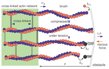
Figure 1: (color online) Schematic representation of an ensemble of actin filaments oriented at $\vartheta=0$ with respect to the normal $\hat{n}$ of an obstacle interface, which may either be a cell membrane or a bacterium. While attached filaments are under tension and pull the interface back, detached filaments are compressed, elongate by polymerization with rate $k_{\text{on}}$ and push the interface forward. All filaments in the brush are firmly anchored in a cross-linked network, whose front advances with velocity $v_{g}$ reducing the free length $l$ of the filaments. Attached filaments detach with stress dependent rate $k_{d}$ and detached filaments attach with constant rate $k_{a}$. $v_{o}$ is the interface velocity in the extracellular medium, and $x$ is the distance between the front of the network and the interface.

Actin polymerization in living cells and extracts is controlled by a complex molecular network Cossart2005 . Nucleation of new filaments, capping of existing ones, exchange of ADP for ATP on actin monomers, buffering of monomers etc. all contribute to that control and have been modeled Carlsson2003 ; mogilner-oster-2003 ; Othmer . Our goal is not to model the full complexity of that biochemical network. Rather we focus on the core process of force generation and force balance ensuing from the interplay between bound pulling filaments and polymerizing pushing filaments, the transition between these two groups and the motion of the whole force generating configuration. This is motivated by recent observations of complex dynamics in simple reconstituted systems: the velocity of beads or pathogens propelled by actin polymerization may oscillate Cossart97 ; Prost2000 ; Prost2005 . Our goal is to describe the dynamics of such biochemically simpler systems and find a robust microscopic description for oscillation mechanisms, which may then be controlled by higher order processes. Such a study is meant to complement investigations based on a continuum approach Prost2000 ; Prost2005 .

We consider a fixed number $N$ of actin filaments Brieher2004 firmly anchored into a rigid cross-linked network, which advances with velocity $v_{g}$; for an illustration see Fig. 1. Filaments of variable length $l$ are either attached to the obstacle interface via a protein complex or detached from it, with time-dependent number distributions denoted by $N_{a}(l,t)$ and $N_{d}(l,t)$, respectively. In the detached state, filaments polymerize at a velocity $v_{p}(l,x)$, which depends on both the polymer length $l$ and the distance $x$ between rigid support and obstacle. Transitions between the two filament populations occur with a constant attachment rate $k_{a}$ and a stress-dependent detachment rate $k_{d}$ Evans-Ritchie-1999 . This results in the evolution equations

$$\frac{\partial}{\partial t}N_{d}-\frac{\partial}{\partial l}\left[\frac{l}{x}v_{g}(l)-v_{p}\right]N_{d} =-k_{a}~{}N_{d}+k_{d}~{}N_{a}\,,$$ (1a)

$$\frac{\partial}{\partial t}N_{a}-\frac{\partial}{\partial l}\left[\frac{l}{x}v_{g}(l)~{}~{}~{}~{}~{}~{}\right]N_{a} =~{}~{}k_{a}~{}N_{d}-k_{d}~{}N_{a}\,.$$ (1b)

The right hand side of Eq. 1 describes attachment and detachment process. The second term on the left hand side accounts for the gain and loss of attached and detached polymers due to the dynamics of the polymer mesh, growing with velocity $v_{g}$, and the polymerization kinetics of the filaments in the brush. The correction factor $l/x$ in front of $v_{g}$ is due to the fact that for bent polymers the rigid network swallows by this amount more in contour length than for straight filaments. This factor is equal to $1$ for $l\leq x$.

Processes contributing to the growth of the rigid polymer mesh are entanglement and crosslinking of filaments in the brush. Both imply a vanishing $v_{g}$ for $l\to 0$, since short polymers do not entangle and crosslinking proteins are unlikley to bind to them. At the same time $v_{g}$ can not grow without bound but must saturate at some value $v_{g}^{\text{max}}$ due to rate limitations for crosslinker binding. This suggests to take the following sigmoidal form

$$v_{g}(l)=v_{g}^{\text{max}}\tanh(l/\bar{l})\,,$$ (2)

with a characteristic length scale $\bar{l}$.

The polymerization rate is proportional to the probability of a gap of sufficient size $d$ ($\approx 2.7$ nm) between the polymer tip and the obstacle for insertion of an actin monomer mogilner-oster:96a . This implies an exponential dependence of $v_{p}$ on the force $F_{\text{d}}$ by which the polymer pushes against the obstacle,

$$v_{p}(l,x)=v_{p}^{\text{max}}\exp\left[-d\cdot F_{\text{d}}(l,x)/k_{\text{B}}T\right]\,.$$ (3)

Here, $v_{p}^{\text{max}}\approx 500$ nm s^-1 mogilner-oster:96a is the free polymerization velocity. For the entropic force $F_{\text{d}}$ we use the results obtained in Ref. gholami-wilhelm-frey:2006 for $D=2,\,3$ spatial dimensions, where we take the accepted value of $\ell_{\text{p}}\approx 15~{}\mu$m persistence_length for the persistence length of F-actin.

The dynamics of the distance $x$ between grafted end of the filament and the obstacle interface (see Fig. 1) is given by the difference of the average $v_{g}$ and the velocity of the obstacle

$$\partial_{t}x=-\frac{1}{N}\int_{0}^{\infty}dl~{}v_{g}(l)~{}\left[N_{a}(l,t)+N_{d}(l,t)\right]$$ (4)

$$+\frac{1}{\zeta}\int_{0}^{\infty}dl~{}\left[N_{a}(l,t)~{}F_{a}(l,x)+N_{d}(l,t)~{}F_{\text{d}}(l,x)\right]\,,$$

where $\zeta$ is an effective friction coefficient of the obstacle. The force $F_{a}(l,x)$ acting on the obstacle interface results from the compliance of the filaments attached to it by some linker protein complex, which we model as springs with spring constant $k_{l}$ and zero equilibrium length. This complex has a nonlinear force-extension relation which we approximate by a piece-wise linear function; for details see the supplementary material. Let $R_{\parallel}\approx l[1-l(D-1)/4\ell_{\text{p}}]$ be the equilibrium length of the filament. Then, the elastic response of filaments experiencing small compressional forces ($x\leq R_{\parallel}$) is approximated by a spring constant $k_{\parallel}=12k_{\text{B}}T~{}\ell_{\text{p}}^{2}/(D-1)l^{4}$ kroy-frey:96 . For small pulling forces ($x\geq R_{\parallel}$), the linker-filament complex acts like a spring with an effective constant $k_{\text{eff}}=k_{l}k_{\parallel}/(k_{l}+k_{\parallel})$. In the strong force regime, the force-extension relation of the filament is highly nonlinear and diverges close to full stretching Marko-Siggia-95 . Therefore, only the linker will stretch out. The complete force-extension relation is captured by

$$F_{a}=\begin{cases}-k_{\parallel}(x-R_{\parallel})\,,&\text{$x\leq R_{\parallel}$ },\\ -k_{\text{eff}}(x-R_{\parallel})\,,&\text{$R_{\parallel}<x<l$ },\\ -k_{l}(x-l)-k_{\text{eff}}(l-R_{\parallel})\,,&\text{$x\geq l$ .}\end{cases}$$ (5)

Finally, we specify the force-dependence of the detachment rate by

$$k_{d}=k_{d}^{0}~{}\exp\left[-d\cdot F_{a}(l,x)/k_{\text{B}}T\right]\,.$$ (6)

Here, $k_{d}^{0}\approx 0.5~{}\text{s}^{-1}$ mogilner-oster-2003 is the detachment rate in the absence of forces and we have followed Ref. Evans-Ritchie-1999 .

Eq. 1a has a singularity at $v_{p}(l_{s})=v_{g}(l_{s})l_{s}/x$ since the coefficient of the derivative of $N_{d}$ with respect to $l$ is zero at $l_{s}$. To illustrate the key physical features at that singularity, we start with the simple equation $\partial_{t}N_{d}-\partial_{l}[v_{g}(l)l/x-v_{p}(l,x)]N_{d}=0$ with $x$ kept constant. Then those parts of the distribution of $N_{d}$ with $l<l_{s}$ will grow and catch up with $l_{s}$ since $v_{g}(l)l/x-v_{p}(l,x)$ is positive there, while the parts with $l>l_{s}$ will shorten towards $l_{s}$. As a consequence the whole distribution will become concentrated at $l_{s}$. To quantify this heuristic argument we expand $v_{g}(l)l/x-v_{p}(l,x)$ up to linear order around $l_{s}$ like $v_{1}(l-l_{s})$ and use the method of characteristics to solve the equation. Starting initially with a Gaussian distribution we obtain $N_{d}(l,t)=c(t)\exp[-(l-\bar{l}(t))^{2}/w(t)^{2}]$ with $c(t)=c_{0}\exp(v_{1}t)$, $\bar{l}(t)=l_{s}+(\bar{l}_{0}-l_{s})\exp(-v_{1}t)$ and $w(t)=w_{0}\exp(-v_{1}t)$. This shows that $N_{d}$ evolves to a monodisperse distribution which is localized around $l_{s}$. Its width decreases exponentially with time while its height grows exponentially. The time scale for this contraction is given by $[\partial_{l}(v_{g}l/x-v_{p})]^{-1}$.

Since the same kind of singularity also occurs in the full set of dynamic equations, Eqs. 1, we may readily infer that $N_{a}$ and $N_{d}$ evolve into delta-functions with that dynamics. This is well supported by simulations, and allows us to continue with the ansatz

$$N_{d}(l,t)=n_{d}(t)~{}\delta(l-l_{d}(t))\,,$$ (7a)

$$N_{a}(l,t)=n_{a}(t)~{}\delta(l-l_{a}(t))\,.$$ (7b)

It defines the dynamic variables $n_{d}(t)$, $l_{d}(t)$, $n_{a}(t)$ and $l_{a}(t)$. Upon inserting Eqs. 7 into Eqs. 1 and Eq. 4, we obtain the following set of ordinary differential equations

$$\partial_{t}l_{d}(t) =~{}v_{p}(l_{d},x)-\frac{l_{d}}{x}v_{g}(l_{d})+k_{d}\frac{n_{a}}{n_{d}}(l_{a}-l_{d})\,,$$ (8a)

$$\partial_{t}l_{a}(t) =-\frac{l_{a}}{x}v_{g}(l_{a})+k_{a}\frac{n_{d}}{n_{a}}(l_{d}-l_{a})\,,$$ (8b)

$$\partial_{t}n_{a}(t) =-k_{d}(l_{a},x)~{}n_{a}(t)+k_{a}~{}n_{d}(t)\,,$$ (8c)

$$\partial_{t}x(t) =\frac{1}{\zeta}\left[n_{a}(t)~{}F_{\text{a}}(l_{a},x)+n_{d}(t)~{}F_{\text{d}}(l_{d},x)\right]$$

$$-\frac{1}{N}[v_{g}(l_{a})~{}n_{a}(t)+v_{g}(l_{d})~{}n_{d}(t)]\,,$$ (8d)

where $n_{d}(t)=N-n_{a}(t)$ since we keep the total number of filaments fixed.

The values of many parameters in the dynamics can be estimated using known properties of actin filaments. We choose the linker spring constant $k_{l}\approx 1$ pN nm^-1 mogilner-oster-2003 and assume $N=200$ mogilner-oster-2003 filaments to be crowded behind the obstacle. A realistic value of the drag coefficient $\zeta$ is $10^{-3}~{}$pN s nm^-1 but results did not change qualitatively for a range from $10^{-5}~{}$pN s nm^-1 to $1~{}$pN s nm^-1.

We have numerically solved Eqs. 8 in both $D=2$ and $D=3$ dimensions, and found the dynamic regimes shown in Fig. 2: stationary states and oscillations. The existence of an oscillatory regime is very robust against changes of parameters within reasonable limits including the spatial dimension. We checked robustness against changes in the parameter values for the number of polymers $N$, $\bar{l}$ (see Eq. 2), $k_{l}$, $v_{p}^{\text{max}}$ and $k_{d}^{0}$, in addition to the examples shown in Fig. 2. In general, we find that oscillations occur for $v_{g}^{\text{max}}\lesssim 500$ nm s^-1 and within a range of values for $k_{a}$. Note that the oscillatory region in parameter space depends on the orientation $\vartheta$ of filaments with respect to the obstacle surface, i.e. oscillating and non-oscillating sub-populations of filaments may coexist in the same network.

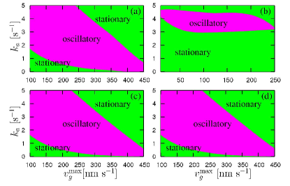
Figure 2: (color online) Phase diagram of Eqs. 8a - 8d outlining stationary and oscillatory regimes with $\zeta=10^{-3}$ pN s nm^-1 for (a-c) and (a) $D=2$, $\vartheta=0$ , (b) $D=2$, $\vartheta=\pi/4$, (c) $D=3$, $\vartheta=0$ and (d) $D=3$, $\vartheta=0$, $\zeta=10^{-5}$ pN s nm^-1. $\bar{l}$=100 nm, all other parameter values are specified in the text.

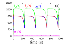
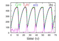
Figure 3: (color online) $x$ , $l_{a}$ , $l_{d}$ (in nm) and $n_{a}$ as a function of time, as obtained from a numerical solutions of Eqs. 8a - 8d with $v_{g}^{\text{max}}=300~{}\text{nm}~{}\text{s}^{-1}$ and (a) $k_{a}=0.143~{}\text{s}^{-1}$ (b) $k_{a}=3.49~{}\text{s}^{-1}$. $D=3$, $\bar{l}$=100 nm in both panels.

Oscillations appear with finite amplitude and period at the lower boundary of the oscillatory region; compare the example shown in Fig. 3a. The stationary state changes stability slightly inside the oscillatory regime and oscillations set in with a finite period. That is compatible with oscillations appearing by a saddle node bifurcation of limit cycles. The upper boundary of the oscillatory region is determined by a Hopf bifurcation. An example of an oscillation close to that bifurcation is shown in Fig. 3b. More details on the phase diagram will be published elsewhere Gholami-Falcke-Frey .

We start with the description of oscillations in the phase with $v_{g}>v_{p}$, i.e., decreasing lengths $x$, $l_{a}$ and $l_{d}$; see Fig. 3. Then the magnitude of pulling and pushing forces increases due to their length-dependence. When the pushing force becomes too strong, an avalanche-like detachment of attached filaments is triggered and the obstacle jerks forward; compare the steep rise in $l_{d}$, $l_{a}$ and $x$ shown in Fig. 3. That causes a just as sudden drop of the pushing force. With low pushing force now, polymerization accelerates and increases the length of detached filaments. The restoring force of attached filaments is weak in this phase due to their small number. Hence, despite of not so strong pushing forces, the obstacle moves forward. In the meantime, some detached filaments attach to the surface such that the average length and number of attached filaments increases as well. When the detached filaments are long enough to notice the presence of the obstacle interface, they start to buckle. This, in turn, increases the pushing force and slows down the polymerization velocity. Therefore, the graft velocity now exceeds the polymerization velocity and the average lengths of attached and detached filaments start to decrease again and the cycle starts anew. The period of oscillations is dependent on the parameter values. It reduces from $240$ s in Fig. 3a to $13$ s in Fig. 3b as $k_{a}$ increases from $0.143~{}\text{s}^{-1}$ to $3.49~{}\text{s}^{-1}$ at $v_{g}^{\text{max}}=300~{}\text{nm}~{}\text{s}^{-1}$.

The oscillations in $x$ correspond to the saltatory motion of the obstacle in the lab frame and the oscillations of its velocity since $v_{g}$ stays essentially constant. An illustration is shown in Fig. 4 for a given set of parameters which leads to oscillations with periods of the order of $100~{}\text{s}$ and velocity of the order of $0.7~{}\mu\text{m}~{}\text{s}^{-1}$. This is in good agreement with the results of experiments on oscillatory Listeria propulsion Cossart97 . The period of velocity oscillations with beads propelled by actin polymerization differs from those of Listeria by one order of magnitude ($8-15$ min Prost2005 ). Periods of that length can be obtained within our model upon using values for $k_{a}$ close to the lower boundary of the oscillatory regime.

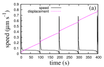
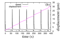
Figure 4: (color online) Velocity and displacement of the obstacle as a function of time with (a) $k_{a}=0.9~{}\text{s}^{-1}$, (b) $k_{a}=1~{}\text{s}^{-1}$. $v_{p}^{\text{max}}=750~{}\text{nm}~{}\text{s}^{-1}$, $v_{g}^{\text{max}}=75~{}\text{nm}~{}\text{s}^{-1}$, $k_{d}^{0}=0.1~{}\text{s}^{-1}$, $\bar{l}$=100 nm $\zeta=10^{-3}$ pN s nm^-1 and $D=3$ in both panels.

We have also studied the system when the network is oriented at an angle $\vartheta=\pi/4$. In this case, the spring constant of the attached filaments parallel to $\hat{n}$ for $D=2$ reads $k_{\parallel}^{-1}(\vartheta)=4\ell_{\text{p}}^{2}[\frac{\epsilon}{2}+\mbox{e}^{-\epsilon/2}-1+\cos 2\vartheta(\frac{1}{4}+\frac{1}{12}\mbox{e}^{-2\epsilon}-\frac{1}{3}\mbox{e}^{-\epsilon/2})-\cos^{2}\vartheta(\mbox{e}^{-\epsilon/2}-1)^{2}]/k_{\text{B}}T$, where $\epsilon=l/l_{p}$ and $R_{\parallel}(\vartheta)=l(1-l/4\ell_{\text{p}})\cos\vartheta$  kroy-frey:96 . For the pushing force of a filament grafted at $\vartheta=\pi/4$, we use the results of the factorization approximation given in Ref. gholami-wilhelm-frey:2006 , which is well valid for a stiff filament like actin. A numerical solution of Eqs. 8a-8d results in the phase diagram shown in Fig. 2(b) with the adapted forms of $F_{\text{d}}$ and $F_{\text{a}}$. The main effect is that one needs higher values for the attachment rates and lower values for $v_{g}$ to obtain oscillations.

In summary, we have presented a simple and generic theoretical description of oscillations arising from the interplay of polymerization driven pushing forces and pulling forces due to binding of actin filaments to the obstacle. The physical mechanism for such oscillations relies on the load-dependence of the detachment rate and the polymerization velocity, mechanical restoring forces and eventually also on the cross-linkage and/or entanglement of the filament network. The oscillations are very robust with respect to changes in various parameters, i.e. are generic in this model. Therefore, complex biochemical regulatory systems supplementing the core process described here may rather stabilize motion and suppress oscillations than generate them.

Oscillations of the velocity were observed during propulsion of pathogens by actin polymerization. There, the core mechanism described here is embedded into a more complex control of polymerization, which e.g. also comprises nucleation of new filaments and capping of existing ones. Hence, the study presented here can not be expected to fully capture all features of such processes. Our results still agree well with respect to velocity spike amplitudes and periods in Listeria experiments reported in Refs. Cossart97 ; Prost2000 . The velocity in between spikes appears to be smaller in experiments than in our simulations. This may be accounted for in our model by including capping of filaments upon dissociation from the obstacle. Periods may also become longer when capping and nucleation were included since it would take longer to restore the pushing force after the avalanche like rupture of attached filaments. Altogether, qualitative and quantitative comparison with experiments suggests that our model may be a promising candidate for a robust mechanism of velocity oscillations in actin-based bacteria propulsion.

We thank R. Straube and V. Casagrande for inspiring discussions. E.F. acknowledges financial support of the German Excellence Initiative via the program ”Nanosystems Initiative Munich (NIM)”. A.G. acknowledges financial support of the IRTG ”Genomics and Systems Biology of Molecular Networks” of the German Research Foundation.

References

- (1) D. Bray, Cell Movements, 2nd ed, Garland, New York.
- (2) J. Plastino and C. Sykes, Curr. Opin. Cell Biol, 17, 62 (2005).
- (3) E. Gouin, M.D. Welch, P. Cossart, Curr. Opin. Microbiol, 8, 35 (2005).
- (4) T.P. Loisel, R. Boujemaa, D. Pantaloni, M.F. Carlier, Nature, 401, 613 (1999).
- (5) Y. Marcy, J. Prost, M.F. Carlier, C. Sykes, Proc. Natl. Acad. Sci. USA 101, 5992 (2004).
- (6) S.H. Parekh, O. Chaudhuri, J.A. Theriot, D.A. Fletcher, Nat. Cell. Biol. 7, 1219 (2005).
- (7) A. Mogilner and G. Oster, Biophy. J. 71, 3030 (1996).
- (8) A. Gholami, J. Wilhelm, E. Frey, Phys. Rev. E. 74 , 41803 (2006).
- (9) T.L. Hill, Proc. Natl. Acad. Sci. USA, 78, 5613 (1981).
- (10) L.A. Cameron et al., Curr. Biol. 11, 130, (2001).
- (11) S.C. Kuo and J.L. McGrath, Nature, 407, 1026 (2000).
- (12) A. Mogilner and G. Oster, Biophy. J. 84, 1591 (2003).
- (13) A.E. Carlsson, Biophys. J. 84, 2907 (2003).
- (14) M.E. Gracheva and H.G. Othmer, Bull. Math. Biol. 66, 167 (2004).
- (15) A. Gholami, M. Falcke, E. Frey (unpublished).
- (16) I. Lasa et al., EMBO J. 16, 1531 (1997).
- (17) F. Gerbal et al., Biophys J. 79, 2259 (2000).
- (18) A. Bernheim-Groswasser, J. Prost, C. Sykes, Biophys J. 89, 1411 (2005).
- (19) A constant number is assumed to simplify matters. It has been shown, however, that a variable number of filaments is not required for propulsion; see e.g. W.M. Brieher, M. Coughlin and T.J. Mitchison, J. Cell Biol. 165 233 (2004)
- (20) E. Evans and K. Ritchie, Biophys. J. 76, 2439 (1999).
- (21) A. Ott et al., Phys. Rev. E 48, R1642 (1993) ; L. LeGoff et al., Phys. Rev. Lett. 89, 258101 (2002).
- (22) K. Kroy and E. Frey, Phys. Rev. Lett. 77, 306 (1996).
- (23) J.F. Marko and E.D. Siggia, Macromol., 28, 8759 (1995).