Instabilities in the time-dependent neutrino disc in Gamma-Ray Bursts

Abstract

We investigate the properties and evolution of accretion tori formed after the coalescence of two compact objects. At these extreme densities and temperatures, the accreting torus is cooled mainly by neutrino emission produced primarily by electron and positron capture on nucleons ($\beta$ reactions). We solve for the disc structure and its time evolution by introducing a detailed treatment of the equation of state which includes photodisintegration of helium, the condition of $\beta$-equilibrium, and neutrino opacities. We self-consistently calculate the chemical equilibrium in the gas consisting of helium, free protons, neutrons and electron-positron pairs and compute the chemical potentials of the species, as well as the electron fraction throughout the disc. We find that, for sufficiently large accretion rates ($\dot{M}\gtrsim 10M_{\odot}$/s), the inner regions of the disk become opaque and develop a viscous and thermal instability. The identification of this instability might be relevant for GRB observations.

1 Introduction

Gamma-Ray Bursts are commonly thought to be produced in relativistic ejecta that dissipate energy by internal shocks however alternative ideas based on the Poynting flux dominated jets are also being proposed (for a review see e.g. Piran 2005; Meszaros 2006; Zhang 2007).

The enormous power released during the gamma-ray burst explosion indicates that a relativistic phenomenon must be involved in creating GRBs (Narayan et al. 1992). The merger of two neutron stars or of a neutron star and a black hole (e.g. NS-NS or NS-BH) has been invoked e.g. by Paczyński (1986); Eichler et al. (1989); Paczyński (1991); Narayan, Paczyński & Piran (1992), as well as the collapse of a massive star, the so called “collapsar” scenario (e.g., Woosley 1993 and Paczyński 1998). In both cases a dense, hot accretion disk is likely to form around a newly born black hole (Witt et al. 1994). In the collapsar scenario, the collapsing envelope of the star accretes onto the newly formed black hole, while a transient debris disk is formed when the NS-NS or NS-BH binary merges (see e.g. Ruffert et al. 1997 for numerical simulations).

The durations of GRBs, which range from milliseconds to over a thousand of seconds, are distributed in two distinct peaks defining two main GRB classes: short ($\leq 2$ sec) and long ($\gtrsim 2$ sec) bursts (Kouvelietou et al. 1993). For some long bursts, signatures of an accompanying supernova explosion have been detected in the afterglow spectra (Stanek et al. 2003; Hjorth et al. 2003), which strongly favors the “collapsar” interpretation for their origin. Furthermore, the GRB positions inferred from the afterglow observations are consistent with the GRBs being associated with the star forming regions in their host galaxies. For short bursts, several pieces of evidence from the analysis of the Swift satellite and follow-up observations (Gehrels et al. 2005; Fox et al. 2005; Villasenor et al. 2005) argue in favor of a binary merger model (Hjorth et al. 2005; Berger et al. 2005).

In the merger scenario, the duration of the burst is comparable to the viscous timescale of the accretion disc whereas in the collapsar scenario, the external reservoir of stellar matter can feed the accretion torus for a much longer timescale. In general, accretion discs powering GRBs are expected to have typical densities of the order of $10^{10-12}$ g cm^-3 and temperatures of $10^{11}$ K within $10-20$ Schwarzschild radii ($R_{\rm S}=2GM/c^{2}$). Thus, accretion proceeds with rates of a fraction to several solar masses per second. In this “hyper-accreting” regime, photons become trapped and are not efficient at cooling the disc. Neutrinos, however, are produced by weak interactions in the dense and hot plasma, releasing the gravitational energy of the accretion flow. These discs go under the name of “neutrino-dominated accretion flows”, or NDAFs.

Over the last several years a number of studies have investigated the structure of these discs (Popham, Woosley & Fryer 1999; Narayan, Piran & Kumar 2001; Kohri & Mineshige 2002; Di Matteo, Perna & Narayan 2002; Surman & McLaughlin 2004; Kohri, Narayan & Piran 2005; Chen & Beloborodov 2006; Gu, Liu & Lu 2006; Liu, Gu & Lu 2007). These models have employed the customary approximation of one-dimensional hydrodynamics (Shakura & Sunyaev 1973), where the effects of MHD viscous stresses are described by the dimensionless parameter $\alpha$, but have been limited to the steady-state approximation of constant $\dot{M}$. Such an assumption is a good approximation when considering the collapsar scenario, where the burst duration is much longer than the viscous time, due to the continuous replenishing of the disc by the collapsing star envelope. However, even in this scenario, recent observations suggest that that engines are “long-lived” (past the torus feeding phase), requiring a time-dependent computation. In the merger scenario, on the other hand, a time-dependent calculation is necessary even for modeling the prompt phase of the burst, since the duration is set by the viscous timescale of the disc.

Recently, a fully time-dependent calculation of the structure of such accretion discs has been presented by Janiuk et al. (2004). The model was suitable for the torus being a results of either the gravitational collapse of a massive stellar core or the compact binary merger. However the structure and evolution of the disk (like in many of the early calculations) was calculated under a number of simplifying assumptions for the composition and the equation of state of the accreting matter. In this paper we improve upon our earlier results in several ways. Besides the requirement of time-dependent calculations, the high density and temperature regime in which the accreting gas lies, implies that both multi-dimensional numerical and semi-analytic calculations for such flows need to include the detailed microphysics. This includes photodisintegration of nuclei, the establishment of statistical equilibrium, neutronization, and the effects of neutrino opacities in the inner regions. Here, we introduce a detailed treatment of the equation of state, and calculate self-consistently the chemical equilibrium in the gas that consists of helium, free protons, neutrons and electron-positron pairs. We compute the chemical potentials of the species, as well as the electron fraction throughout the disk using the assumption of the equilibrium between the beta processes. Our EOS equations include, self-consistently, the contribution of the neutrino trapping to the beta equilibrium. Another important addition compared to our previous work (Janiuk et al. 2004) is the inclusion of photodisintegration of helium. The presence of this term can affect the energy balance in the inner, opaque (to neutrinos as well as photons) region of the flow and, as it will be shown, it eventually produces a thermal and viscous instability in those regions. This is especially relevant since the GRB phenomenology requires a variable energy output.

Other time-dependent disc studies of binary mergers or collapsars have been performed in 2D using hydrodynamical simulations (e.g. MacFadyen & Woosley 1999; Ruffert & Janka 1999; Lee et al. 2002; Rosswog et al. 2004; Lee, Ramirez-Ruiz & Page 2005) and, most recently, in 3-D simulations (Setiawan et al. 2005). Also, MHD simulations of the GRB central engine have been performed, showing that the magnetic field possibly plays an important role in the generation of a GRB jet (Proga et al. 2003; Fujimoto et al. 2006). The advantage of our calculations is that, whilst including all the relevant physics to calculate the equation of state, the structure and stability of the accretion disc, we are able to study a much larger range of parameter space and allow our calculations to evolve beyond what can be reached in higher dimensional calculation and comparable to at least the short-burst durations.

The paper is organized as follows. In Section 2 we describe the basic assumptions of the model and the method used in the initial stationary and subsequent time-dependent numerical simulations. In Section 3 we discuss the structure of the hyperaccreting disc for various values of the initial accretion rate, and study the time evolution of its density and temperature, as well as the resulting neutrino lightcurve. We also discuss the physical origin of the instabilities in the disc, and we compare our model and results with the recent 2D and 3D simulations. We summarize our results in Section 4.

2 Neutrino-cooled accretion disks

In this Section, we describe how we improve upon our previous time-dependent calculation (Janiuk et al. 2004) by computing self-consistently the equation of state of the extremely dense matter by solving the balance of the $\beta$ reaction rates. This allows us to determine the chemical potentials of electrons, protons and neutrons, as well as the electron fraction, in the initial disc configuration and throughout its evolution.

2.1 Initial disc configuration: 1-D Hydrodynamics

We start by considering a steady-state model of an accretion disc around a Schwarzschild black hole - formed as a remnant structure either after a compact binary merger, or in a collapsar after the birth of a black hole (for a recent calculation in Kerr spacetime see Chen & Beloborodov 2006). Throughout our calculations we use the vertically integrated equations and hence derive a vertically averaged disc structure. We write the surface density of the disk as $\Sigma=H\rho$, where $\rho$ is the density and where the disk half thickness (or disk height) is given by $H=c_{s}/\Omega_{K}$. Here the sound speed is defined by $c_{s}=\sqrt{P/\rho}$ and $\Omega_{\rm K}=\sqrt{GM/r^{3}}$ is the Keplerian angular velocity with $P$ the total pressure. We note that, at very high accretion rates, the disc becomes moderately geometrically thick ($H\sim 0.5r$) in regions where neutrino cooling becomes inefficient and advection dominates. Our ’slim disk’ approximation neglects terms $\sim(H/r)^{2}$ and assumes that the fluid is in Keplerian rotation. For the disc viscous stress we use the standard $\alpha$ viscosity prescription of Shakura & Sunyaev (1973) where the stress tensor is proportional to the pressure:

$$\tau_{r\varphi}=-\alpha P.$$ (1)

We adopt a value of $\alpha=0.1$

We set the inner radius of the disc at 3 $R_{\rm S}$, while the outer radius is at 50 $R_{\rm S}$. The initial mass of such a disc is about $0.35M_{\odot}$ for an accretion rate $\dot{M}=1~{}M_{\odot}$/s. Throughout the calculations we adopt a black hole mass of $M=3M_{\odot}$.

2.2 The equation of state

We assume that the torus consists of helium, electron-positron pairs, free neutrons and protons. The total pressure is contributed by all particle species in the disc, and the fraction of each species is determined by self-consistently solving the balance of the beta reaction rates. In the equation of state we take into account the pressure due to the free nuclei and pairs, helium, radiation and the trapped neutrinos:

$$P=P_{\rm nucl}+P_{\rm He}+P_{\rm rad}+P_{\nu}\;.$$ (2)

The component $P_{\rm nucl}$ includes free neutrons, protons, and the electron-positron pair gas in beta equilibrium:

$$P_{\rm nucl}=P_{\rm e-}+P_{\rm e+}+P_{\rm n}+P_{\rm p}$$ (3)

with

$$P_{\rm i}={2\sqrt{2}\over 3\pi^{2}}{(m_{i}c^{2})^{4}\over(\hbar c)^{3}}\beta_{i}^{5/2}\left[F_{3/2}(\eta_{\rm i},\beta_{\rm i})+{1\over 2}\beta_{\rm i}F_{5/2}(\eta_{\rm i},\beta_{\rm i})\right]\;,$$ (4)

where $F_{\rm k}$ are the Fermi-Dirac integrals of the order $k$, and $\eta_{\rm e}$, $\eta_{\rm p}$ and $\eta_{\rm n}$ are the reduced chemical potentials of electrons, protons and neutrons in units of $kT$, respectively (where $\eta_{i}=\mu_{i}/kT$, also known as the degeneracy parameter, where $\mu_{i}$ the standard chemical potential) calculated from the chemical equilibrium condition (§ 2.3). The reduced chemical potential of positrons is $\eta_{\rm e+}=-\eta_{\rm e}-2/\beta_{\rm e}$ and the relativity parameters of the species $i$ are defined as $\beta_{\rm i}=kT/m_{\rm i}c^{2}$.

Under the physical conditions in the torus, helium is generally non-relativistic and non-degenerate; therefore, its pressure is given by:

$$P_{\rm He}=n_{\rm He}kT,$$ (5)

where $n_{\rm He}$ is the number density of helium. This is defined as:

$$n_{\rm He}={1\over 4}n_{b}(1-X_{\rm nuc})\;,$$ (6)

and the fraction of free nucleons is given by

$$X_{\rm nuc}=295.5\rho_{10}^{-3/4}T_{11}^{9/8}\exp(-0.8209/T_{11}),$$ (7)

with $T_{11}$ the temperature in unit of 10¹¹ K (e.g. Qian & Woosley 1996; Popham et al. 1999).

The radiation pressure is given by:

$$P_{\rm rad}={1\over 3}{\pi^{2}\over 15}{(kT)^{4}\over(\hbar c)^{3}}.$$ (8)

When neutrinos become trapped in the disc, the neutrino pressure is non-zero. Following the treatment of photon transport under the two-stream approximation (Popham & Narayan 1995; Di Matteo et al. 2002), we have

$$P_{\nu} = {7\over 8}{\pi^{2}\over 15}{(kT)^{4}\over 3(\hbar c)^{3}}\sum_{i=e,\mu,\tau}{{1\over 2}(\tau_{a,\nu_{i}}+\tau_{s})+{1\over\sqrt{3}}\over{1\over 2}(\tau_{a,\nu_{i}}+\tau_{s})+{1\over\sqrt{3}}+{1\over 3\tau_{a,\nu_{i}}}}$$ (9)

$$\equiv {7\over 8}{\pi^{2}\over 15}{(kT)^{4}\over 3(\hbar c)^{3}}b,$$

where $\tau_{\rm s}$ is the scattering optical depth due to the neutrino scattering on free neutrons and protons and $\tau_{\rm a,\nu_{e}}$ and $\tau_{\rm a,\nu_{\mu}}$ are the absorptive optical depths for electron and muon neutrinos, respectively (see§2.3). The contribution from tau neutrinos is the same as that from muon neutrinos. These optical depths and neutrino absorption processes (which are the reverse of the emission processes) are discussed in more detail in the Appendix.

In the disc we have to consider both the neutrino transparent and opaque regions, as well as the transition between the two. In the transparent case, the neutrinos are not thermalized and the chemical potential of neutrinos is negligible. On the other hand, when neutrinos are totally trapped, the chemical equilibrium condition yields: $\mu_{\rm e}+\mu_{\rm p}=\mu_{\rm n}+\mu_{\nu}$. The chemical potential of neutrinos is a parameter depending on how much neutrinos and anti-neutrinos are trapped, and assuming that the number densities of the trapped neutrinos and anti-neutrinos are the same, $\mu_{\nu}$ can be set to zero. In order to determine the distribution function of the partially trapped neutrinos, in principle one should solve the Boltzmann equation. To simplify this problem, we use here a ”gray body” model, and we introduce a blocking factor $b=\sum_{i=e,\mu,\tau}b_{i}$ to describe the extent to which neutrinos are trapped (see e.g. Sawyer 2003). In terms of this factor, we write the distribution function of neutrinos as

$$\widetilde{f}_{\nu_{i}}(p)=\frac{b_{i}}{\exp(pc/kT)+1}=b_{i}f_{\nu_{i}},\,\,\,(0\leq b_{i}\leq 1).$$ (10)

This simplified assumption is consistent with the two-stream approximation which we adopt here (Eq. 9).

2.3 Composition and chemical equilibrium

The equilibrium state of the gas in the accreting torus is completely determined by the chemical potentials of neutrons, protons and electrons ($\eta_{n},\eta_{p},\eta_{e}$), and the trapping factor of neutrinos ($b$) which is related to the optical depths of neutrinos (cf. Eq. 9). For a given baryon number density, $n_{\rm b}$, temperature $T$, and a value for accretion rate $\dot{M}$ and viscous constant $\alpha$, the chemical potentials, or equivalently the ratio of free protons $x=n_{p}/n_{b}$, are determined from the condition of equilibrium between the transition reactions from neutrons to protons and from protons to neutrons. These reactions are:

$$p+e^{-}\to n+\nu_{\rm e}$$ (11)

$$p+\bar{\nu}_{\rm e}\to n+e^{+}$$ (12)

$$p+e^{-}+\bar{\nu}_{e}\to n$$ (13)

$$n+e^{+}\to p+\bar{\nu}_{\rm e}$$ (14)

$$n\to p+e^{-}+\bar{\nu}_{\rm e}$$ (15)

$$n+\nu_{\rm e}\to p+e^{-}$$ (16)

Therefore we have to calculate the ratio of protons that will satisfy the balance:

$$n_{\rm p}(\Gamma_{p+e^{-}\to n+\nu_{\rm e}}+\Gamma_{p+\bar{\nu}_{\rm e}\to n+e^{+}}+\Gamma_{p+e^{-}+\bar{\nu}_{\rm e}\to n})$$

$$=n_{\rm n}(\Gamma_{n+e^{+}\to p+\bar{\nu}_{\rm e}}+\Gamma_{n\to p+e^{-}+\nu_{\rm e}}+\Gamma_{n+\nu_{\rm e}\to p+e^{-}})\;.$$ (17)

The reaction rates are the sum of forward and backward rates and are given in the Appendix (see also Kohri, Narayan and Piran 2005).

These are supplemented by two additional conditions: the conservation of the baryon number, $n_{n}+n_{p}=n_{b}\times X_{\rm nuc}$, and charge neutrality (Yuan 2005):

$$n_{\rm e}=n_{e^{-}}-n_{e^{+}}=n_{\rm p}+n_{\rm e}^{0}\;,$$ (18)

which says that the net number of electrons is equal to the number of free protons plus the number of protons in helium:

$$n_{\rm e}^{0}=2n_{\rm He}=(1-X_{\rm nuc}){n_{\rm b}\over 2}.$$ (19)

The number density of fermions under arbitrary degeneracy is determined by the following equations:

$$n_{\rm i}={\sqrt{2}\over\pi^{2}}\left({m_{i}c^{2}\over\hbar c}\right)^{3}\beta_{\rm i}^{3/2}\left[F_{1/2}(\eta_{\rm i},\beta_{\rm i})+\beta_{\rm i}F_{3/2}(\eta_{\rm i},\beta_{\rm i})\right].$$ (20)

Finally, the electron fraction is defined as:

$$Y_{\rm e}={n_{\rm e^{-}}-n_{\rm e^{+}}\over n_{\rm b}}$$ (21)

(Note that this is different from $Y_{\rm e}=1/(1+n_{\rm n}/n_{\rm p})$, which is only valid for free n-p-e gas.)

2.4 Neutrino cooling

The processes that are responsible for the neutrino emission in the disc are electron-positron pair annihilation ($e^{-}+e^{+}\to\nu_{\rm i}+\bar{\nu}_{\rm i}$), bremsstrahlung ($n+n\to n+n+\nu_{\rm i}+\bar{\nu}_{\rm i}$), plasmon decay ($\tilde{\gamma}\to\nu_{\rm e}+\bar{\nu}_{\rm e}$) and URCA process (reactions 11, 14 and 15). The first two processes produce neutrinos of all flavors, while the other produce only electron neutrinos and anti-neutrinos.

The cooling rate due to pair annihilation is expressed as:

$$q_{\rm e^{+}e^{-}}=q_{\nu_{\rm e}}+q_{\nu_{\mu}}+q_{\nu_{\tau}}$$ (22)

where the cooling rates for all three neutrino flavors are calculated by means of Fermi-Dirac integrals and are given in the Appendix.

The cooling rate due to nucleon-nucleon bremsstrahlung (in erg/cm³/s) is given by:

$$q_{\rm brems}=3.35\times 10^{27}\rho_{10}^{2}T_{11}^{5.5}\;,$$ (23)

where $\rho_{10}$ is the baryon density in units of 10¹⁰ g/cm³ and $T_{11}$ is temperature in units of 10¹¹ K.

The cooling rate due to the plasmon decay (in erg/cm³/s) is:

$$q_{\rm plasmon}=1.5\times 10^{32}T_{11}^{9}\gamma_{p}^{6}e^{-\gamma_{p}}(1+\gamma_{p})\left(2+{\gamma_{p}^{2}\over 1+\gamma_{p}}\right)\;,$$ (24)

where $\gamma_{p}=5.565\times 10^{-2}\sqrt{(\pi^{2}+3(\mu_{e}/kT)^{2})/3}$.

The cooling rate due to the URCA reactions is given by the three emissivities:

$$q_{\rm urca}=q_{p+e^{-}\to n+\nu_{\rm e}}+q_{\rm n+e^{+}\to p+\bar{\nu}_{\rm e}}+q_{n\to p+e^{-}+\bar{\nu}_{\rm e}}\;.$$ (25)

The emissivities are given in the Appendix.

Note that the blocking factor of the trapping neutrinos is used only for the emissivities of the URCA reactions. For simplicity, we neglect the blocking effects of neutrinos when calculating the emissivities for the electron-positron pair annihilation. Two reasons make this approximation reasonable: the emissivities for the electron-positron pair annihilation is much smaller than those of the URCA reactions, and the electron-positron pair annihilation does not change the electron fraction which sensitively affects the EOS.

Each of the above neutrino emission process has a reverse process, which leads to neutrino absorption. These are given by Equations 12, 13 and 16. Therefore we introduce the absorptive optical depths for neutrinos given by:

$$\tau_{\rm a,\nu_{i}}={H\over 4{7\over 8}\sigma T^{4}}q_{\rm a,\nu_{i}}$$ (26)

where absorption of the electron neutrinos is determined by:

$$q_{\rm a,\nu_{e}}=q_{\nu_{e}}^{\rm pair}+q_{\rm urca}+q_{\rm plasm}+{1\over 3}q_{\rm brems}$$ (27)

and for the muon neutrinos:

$$q_{\rm a,\nu_{\mu}}=q_{\nu_{\mu}}^{\rm pair}+{1\over 3}q_{\rm brems}\;.$$ (28)

In addition, the free escape of neutrinos from the disc is limited by scattering. The scattering optical depth is given by:

$$\tau_{\rm s} = \tau_{\rm s,p}+\tau_{\rm s,n}$$

$$= 24.28\times 10^{-5}\left[\left({kT\over m_{\rm e}c^{2}}\right)^{2}H\left(C_{\rm s,p}n_{\rm p}+C_{\rm s,n}n_{\rm n}\right)\right]$$

where $C_{\rm s,p}=(4(C_{V}-1)^{2}+5\alpha^{2})/24$, $C_{\rm s,n}=(1+5\alpha^{2})/24$, $C_{\rm V}=1/2+2\sin^{2}\theta_{\rm C}$, with $\alpha=1.25$ and $\sin^{2}\theta_{\rm C}=0.23$.

The neutrino cooling rate is then given by

$$Q^{-}_{\nu}={{7\over 8}\sigma T^{4}\over{3\over 4}}\sum_{i=e,\mu}{1\over{\tau_{\rm a,\nu_{i}}+\tau_{\rm s}\over 2}+{1\over\sqrt{3}}+{1\over 3\tau_{\rm a,\nu_{i}}}}\;.$$ (30)

2.5 Energy and momentum Conservation

The hydrodynamic equations we solve to calculate the disc structure are the standard mass, energy and momentum conservation.

Making use of the standard disk equations, the vertically integrated viscous heating rate (per unit area) over a half thickness $H$ is given by:

$$F_{\rm tot}={3GM\dot{M}\over 8\pi r^{3}}f(r)$$ (31)

where the Newtonian boundary condition is assumed: $f(r)=1-\sqrt{r_{min}/r}$. Note that in the time-dependent calculations, instead of Eq. 31, we will solve the viscous diffusion equation (Eq. 44).

Using mass and momentum conservation $\dot{M}=4\pi\rho RHv_{r}\approx 6\pi\nu\rho H$ where $v_{r}\approx(3\nu)/(2r)$ and $\nu=(2P\alpha)/(3\rho\Omega)$ is the kinematic viscosity. The viscous heating rate can be written in terms of $\alpha$,

$$Q^{+}_{\rm visc}={3\over 2}\alpha\Omega HP.$$ (32)

Cooling in the disc is due to advection, radiation and neutrino emission. The advective cooling in a stationary disc is determined approximately as:

$$Q^{-}_{\rm adv}=\Sigma v_{r}T{dS\over dr}=q_{\rm adv}{\alpha PHT\over\Omega\rho r^{2}}S\;,$$ (33)

where $q_{\rm adv}\propto d\ln S/d\ln r\propto(d\ln T/d\ln r-(\Gamma_{3}-1)d\ln\rho/d\ln r)\approx const$ and we adopt the value of 1.0. The entropy density $S$ is the sum of four components:

$$S=S_{\rm nucl}+S_{\rm He}+S_{\rm rad}+S_{\nu}\;.$$ (34)

The entropy density of the gas of free protons, neutrons and electron-positron pairs is given by:

$$S_{\rm nucl}=S_{\rm e^{-}}+S_{\rm e^{+}}+S_{\rm p}+S_{\rm n}$$ (35)

where

$$\frac{S_{\rm i}}{k}={1\over kT}(\epsilon_{i}+P_{\rm i})-n_{\rm i}\eta_{\rm i}$$ (36)

and

$$\epsilon_{i}={2\sqrt{2}\over 3\pi^{2}}{(m_{\rm i}c^{2})^{4}\over(\hbar c)^{3}}\beta_{\rm i}^{5/2}\left[F_{3/2}(\eta_{\rm i},\beta_{\rm i})+\beta_{\rm i}F_{5/2}(\eta_{\rm i},\beta_{\rm i})\right]$$ (37)

is the energy density of electrons, positrons, protons or neutrons, $P_{\rm i}$ is their pressure, given by Equation 4, $n_{\rm i}$ are the number densities and $\eta_{\rm i}$ are the chemical potentials.

The entropy density of helium is given by:

$$S_{\rm He}=n_{\rm He}\left[{5\over 2}+{3\over 2}\log(m_{\rm He}{kT\over m_{\rm e}c^{2}}{1\over 2\pi}-\log n_{\rm He})\right]\;,$$ (38)

for $n_{\rm He}>0$.

The entropy density of radiation is

$$S_{\rm rad}=4{P_{\rm rad}\over kT}\;,$$ (39)

while for neutrinos we have

$$S_{\nu}=4{P_{\nu}\over kT}.$$ (40)

In the initial disc configuration we assume that $q_{\rm adv}$ is approximately constant and of order of unity, but in the subsequent time-dependent evolution the advection term is calculated with the appropriate radial derivatives.

For the case of photon and electron-positron pairs in the plasma the radiative cooling is equal to:

$$Q^{-}_{\rm rad}={3P_{\rm rad}c\over 4\tau}={11\sigma T^{4}\over 4\kappa\Sigma}$$ (41)

where we adopt the Rosseland-mean opacity $\kappa=0.4+0.64\times 10^{23}\rho T^{-3}$  [cm²g^-1].

An important term in the cooling and heating balance in the disc is due to photodisintegration of $\alpha$ particles, with rate:

$$Q_{\rm photo}=q_{\rm photo}H$$ (42)

where

$$q_{\rm photo}=6.28\times 10^{28}\rho_{10}v_{r}{dX_{\rm nuc}\over dr}$$ (43)

and $X_{\rm nuc}$ is given by Equation 7. Finally, in order to calculate the initial stationary configuration, we solve the energy balance: $F_{\rm tot}=Q^{+}_{\rm visc}=Q^{-}_{\rm adv}+Q^{-}_{\rm rad}+Q^{-}_{\nu}+Q_{\rm photo}$.

2.6 Time evolution

After solving for the initial disc configuration, we allow the density and temperature to vary with time. We solve the time-dependent equations of mass and angular momentum conservation in the disc:

$${\partial\Sigma\over\partial t}={1\over r}{\partial\over\partial r}\left[3r^{1/2}{\partial\over\partial r}(r^{1/2}\nu\Sigma)\right]$$ (44)

and the energy equation:

$${\partial T\over\partial t}+v_{\rm r}{\partial T\over\partial r}={T\over\Sigma}{4-3\chi\over 12-9\chi}\left({\partial\Sigma\over\partial t}+v_{\rm r}{\partial\Sigma\over\partial r}\right)$$ (45)

$$+{T\over PH}{1\over 12-9\chi}(Q^{+}-Q^{-}).$$

where $\chi=(P-P_{\rm rad})/P$. The cooling term $Q^{-}$ consists of radiative and neutrino cooling, given by Equations (41) and (30). Advection is included in the energy equation via the radial derivatives. The cooling term due to photodisintegration of helium now must be proportional to the full time derivative of $X_{\rm nuc}$ (cf. Eq. 43) :

$$Q_{\rm photo}\propto v_{\rm r}{\partial X_{nuc}\over\partial r}+{\partial X_{\rm nuc}\over\partial t}.$$ (46)

2.7 Numerical method

The initial configuration of the disc is calculated by means of the Newton-Raphson method, iterated with the hydrostatic equilibrium condition. We interpolate over the matrix of pre-calculated results for the equation of state (pressure and entropy) and neutrino cooling rate ( the number of points is 1024x1024). The Fermi-Dirac integrals are calculated using the mixture of Gauss-Legendre and Gauss-Laguerre quadratures (Aparicio 1998).

Having determined the initial radial profiles of density and temperature, as well as the other quantities at time $t=0$, we start the time evolution of the disc. We solve the set of Equations (44), (2.6) and (46) using the convenient change of variables $y=2r^{1/2}$ and $\Xi=y\Sigma$, at fixed radial grid, equally spaced in $y$ (see Janiuk et al. 2002 and references therein). The number of radial zones is set to 200, which we found to be an adequate resolution. After determining the solutions for the first 100 time steps by the fourth-order Runge-Kutta method, we use the Adams-Moulton predictor-corrector method with an adaptive time step. The code used an explicit communication model that is implemented with the standardized MPI communication interface and can be run on multiprocessor machines.

We choose the no-torque inner boundary condition, $\Sigma_{\rm in}=T_{\rm in}=0$ (see Abramowicz & Kato 1989). The outer boundary of the disc is done by adding an extra “dead-zone” to the computational domain, which accounts for the disk expansion and conservation of angular momentum.

3 Results

We first analyze the pressure, entropy and neutrino cooling rate distributions for a given temperature and baryon density in the gas. Then, we show the disc structure for a converged static disc model and finally we show examples of time evolution of the neutrino luminosity, density, temperature and electron fraction for given sets of parameters.

3.1 EOS solutions for a given temperature and density

In Figure 1 and 2 we plot the results of the numerically calculated equation of state for the hot and dense matter. The plots show the dependence of the electron fraction, pressure, entropy and neutrino cooling rate on temperature and density, respectively.

In the upper panels, we show the neutrino cooling rate. At low temperatures, below $T=m_{\rm e}c^{2}\sim 5\times 10^{9}K$, there are almost no positrons and free nucleons. Therefore the neutrino emission processes switch off, and the cooling of the gas is either due to advection, or, when the matter becomes transparent to photons, radiative cooling overtakes. For larger temperatures, the neutrino emission rate increases up to the temperature of about $\sim 5\times 10^{11}$ K. For very high temperatures, the optical depths for neutrinos increase very rapidly ($\tau\propto T^{5}$, see Eq. (7) in Di Matteo et al. 2002). Therefore the neutrino cooling rate decreases at high temperatures (Eq. 30). On the other hand, for a given temperature (e.g. $T\sim 10^{11}$ K), the neutrino cooling rate does not sensitively depend on density. It varies by one order of magnitude in the range of $10^{8}\leq\rho\leq 10^{14}$ g/cm³, where the optical depth is $\tau\sim 100$.

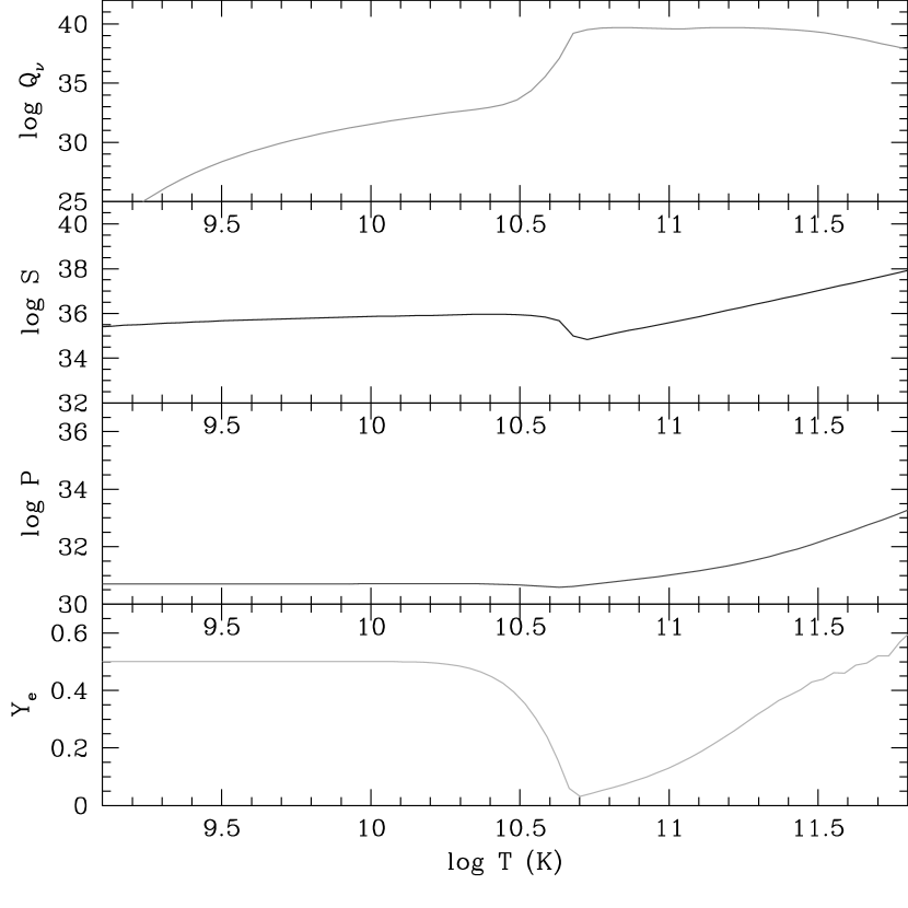
Figure 1: The dependence of the electron fraction (bottom), pressure (middle bottom), entropy (middle upper) neutrino cooling rate (upper panel) on temperature, for the constant density $\rho=10^{12}$ g/cm³. The accretion rate is $\dot{M}=1~{}M_{\odot}$/s. The pressure and neutrino cooling are in cgs units and the entropy is in units of $k_{\rm B}$ cm^-3.

The middle panels of Figures 1 and 2, show the entropy and pressure as a function of temperature and density. At low temperatures, the entropy of gas is not important. The highly degenerate electrons do not give contribution to the entropy, while they are a dominant term in the pressure, which is therefore independent of temperature up to $T\sim 5\times 10^{10}$ K. When the temperature increases, helium becomes disintegrated into free nucleons at energy comparable to the binding energy of helium, and after that the radiation (including photons and electron-positron pairs) contributes mainly to the total entropy and pressure. Therefore, both these quantities rise with temperature. At high densities, the entropy is dominated by neutrons.

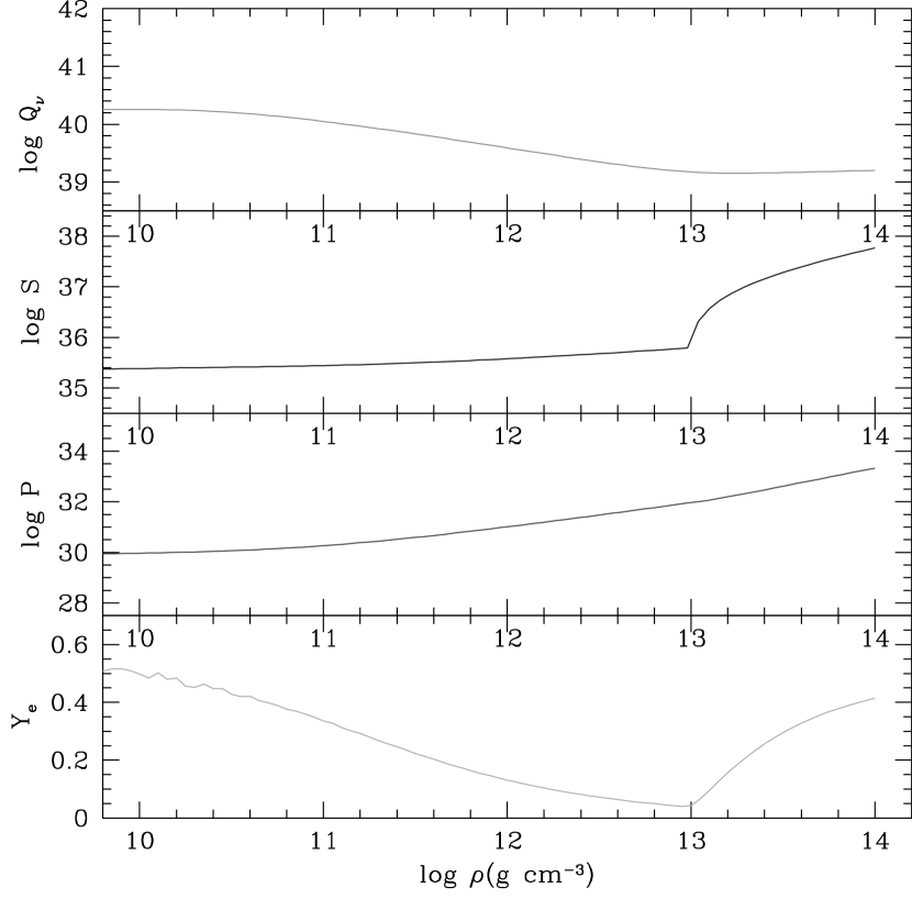
Figure 2: The dependence of the electron fraction (bottom), pressure (middle bottom), entropy (middle upper) and neutrino cooling rate (upper panel) on density, for the constant temperature $T=10^{11}$ K. The accretion rate is $\dot{M}=1~{}M_{\odot}$/s. The pressure and neutrino cooling are in cgs units and the entropy is in units of $k_{\rm B}cm^{-3}$.

Finally, the electron fraction is shown in the bottom panel of Figures 1 and 2. At low temperatures, the electron fraction is equal to 0.5, it then decreases sharply as the helium nuclei become disintegrated. As the temperature further increases, positrons appear as the electrons become non-degenerate. The positron capture again increases the electron fraction (see Fig.1).

The electron fraction changes significantly as a function of density for $T>10^{10}K$ (in Fig.2, $T=10^{11}K$). At low densities, the torus consists of free neutrons and protons and $Y_{\rm e}$ is close to 0.5 (see also Eq. 7). As density increases, $Y_{\rm e}$ decreases to satisfy the beta-equilibrium among the free n-p-e gas. Above some density (when the temperature is high enough, e.g. for Fig. 2, $\rho_{\rm He}\approx 10^{13}$g cm^-3) helium starts forming. Therefore $Y_{\rm e}$ has a kink and stars rising steeply, asymptotically approaching 0.5 as the torus consists of plenty of ionized helium and some electrons to keep charge neutrality.

3.2 The steady-state disc structure

In Figures 3 and 4 we show the profiles of density and temperature in the stationary accretion disk model for three accretion rates: $1~{}M_{\odot}$/s, $10~{}M_{\odot}$/s and $12~{}M_{\odot}$/s. In general, the temperature and density profiles both increase inward. However, for $\dot{M}=12M_{\odot}$/s, a distinct branch of solutions is reached, which appears different than the so-called “NDAF” branch (see Kohri & Mineshige 2002). The density and temperature profiles for this high accretion rate differ also from what was found in previous work (Di Matteo et al. 2002; Janiuk et al. 2004). Due to a more detailed equation of state, in which we allow for a partial degeneracy of nucleons and electrons as well as neutrino trapping, our solutions reach densities as high as $10^{12}$ g/cm³ in the innermost radii of the disc. The temperature in this inner disc part is in the range $4\times 10^{10}-1.25\times 10^{11}$ K, depending on the accretion rate. For the hottest disk model, a local peak in the density forms around $7-8R_{\rm S}$, while below that radius the density decreases. Between $\sim$ 3.5 and 7 $R_{\rm S}$, the plasma becomes much hotter and less dense than outside of this region. This means that the macroscopic state of the system is different here due to an abrupt change in the heat capacity. In order to check what is the reason for this transition, we investigate the pressure distribution in the disk.

Figure 3: The baryon density as a function of the disc radius, calculated in the stationary solution. The accretion rate is $\dot{M}=1~{}M_{\odot}$/s (solid line), $\dot{M}=10~{}M_{\odot}$/s (long dashed line) and $\dot{M}=12~{}M_{\odot}$/s (short dashed line) .

Figure 4: The temperature as a function of the disc radius, calculated in the stationary solution. The accretion rate is $\dot{M}=1~{}M_{\odot}$/s (solid line), $\dot{M}=10~{}M_{\odot}$/s (long dashed line) and $\dot{M}=12~{}M_{\odot}$/s (short dashed line) .

The profile of the pressure is shown in Fig. 5. The dominant term in the total pressure is due to the nucleons, while the radiation pressure (including electron-positron pairs) is always several orders of magnitude smaller. The neutrino pressure is large in the inner disc, once it gets optically thick to neutrinos (i.e. for $\dot{M}\geq 10M_{\odot}$/s). A significant contribution to the pressure is due to helium at densities high enough for helium to form, albeit at temperatures low enough such that its nuclei are not fully disintegrated. For the largest accretion rate shown, in the region of the temperature excess and inverse density gradient ($3.5-7R_{\rm S}$), the total pressure distribution flattens. The helium pressure is now vanishingly small due to the complete photodisintegration, and the nuclear pressure is slightly decreased due to the composition change: smaller number density of neutrons and larger number density of protons. The substantial contribution to the pressure is now given by the neutrinos (large optical depths; see below) and radiation pressure (increased number of electron-positron pairs). From the comparison of Figures 3, 4 and the bottom panel of Figure 5, it can be seen that the total pressure becomes locally correlated with temperature and anticorrelated with density, thus consituting an unstable phase.

Figure 5: The pressure components as a function of the disc radius, calculated in the stationary solution for the three accretion rate values: $\dot{M}=1~{}M_{\odot}$/s (upper panel), $\dot{M}=10~{}M_{\odot}$/s (middle panel) and $\dot{M}=12~{}M_{\odot}$/s (bottom panel) . The total pressure is marked by the solid line, and its components are: nuclear (gas) pressure (long dashed line), radiation pressure (short dashed line), helium pressure (dotted line) and neutrino pressure (dot-dashed line).

Figure 6: The neutrino optical depths due to scattering ($\tau_{\rm s}$, solid line) and absorption ($\tau_{\rm a,e}$ for electron neutrinos, long dashed line, and $\tau_{a,\mu}$ for muon neutrinos, short dashed line) as a function of radius for $\dot{M}=1M_{\odot}/s$ (upper panel), $\dot{M}=10M_{\odot}/s$ (middle panel) and for $\dot{M}=12M_{\odot}/s$ (bottom panel). The sum of the three quantities is the total optical depth ($\tau_{\rm tot}$, dotted line).

In Figure 6 we show the neutrino optical depths due to scattering and absorption. The total optical depth in the outer disc is typically dominated by scattering processes, while in the inner disc absorption processes take over for very high accretion rates. For $\dot{M}=1M_{\odot}$/s only the very inner disk radii have optical depth close to 1. For $\dot{M}=12M_{\odot}$/s, in the radial strip of $\sim 3.5-7R_{\rm S}$ the disk is optically thick with absorptive optical depth for electron neutrinos exceeding the scattering term and reaching values of the order of 100.

3.2.1 Composition and Chemical potentials

In Figure 7 we show the distribution of the reduced chemical potentials of protons, electrons and neutrons throughout the disc. Reduced electron chemical potentials much larger than unity (indicating strong electron degeneracy) are found in the inner disc parts for $\dot{M}=10M_{\odot}$/s and $\dot{M}=12M_{\odot}$/s, whereas for 1 $M_{\odot}$/s electrons are only slightly degenerate. For the highest accretion rate, the maximum degeneracies correspond to the radius of the local peak in the density (cf. Fig. 3) and the excess of helium number density (cf. Fig. 8). Below this radius, the species become non-degenerate again, contributing to the increase of the electron fraction (cf. Fig. 9).

Figure 7: The chemical potentials of neutrons ($\eta_{\rm n}$, solid line), electrons ($\eta_{\rm e}$, dashed line) and protons ($\eta_{\rm p}$, dotted line) as a function of the disc radius, calculated in the stationary solution. The accretion rate is $\dot{M}=1~{}M_{\odot}$/s (triangles), $\dot{M}=10~{}M_{\odot}$/s (squares) and $\dot{M}=12~{}M_{\odot}$/s (circles).

In Figure 8 we plot the mass fraction of free nucleons as a function of radius for $\dot{M}=12M_{\odot}$/s, 10 and $1M_{\odot}$/s. As the Figure shows, in the outer regions, $X_{\rm nuc}$ increases as the radius decreases, while the temperature and density increase (Fig. 3 and Fig. 4). Consistent with the behavior of $Y_{\rm e}$ (Fig.2), $X_{\rm nuc}$ subsequently turns around (decreases) at radii where the density is high enough for significant helium formation. This trend is reversed sharply for highest accretion rates, when the temperature in the disk is high enough (Fig.4) for helium to be fully dissociated. In consequence, the number density of alpha particles increases at $\sim 7-12R_{\rm S}$ and sharply decreases at lower radii. A similar, but far less pronounced fluctuation in $X_{\rm nuc}$ is seen at smaller radii for the case of $\dot{M}=10M_{\odot}$/s. For smallest accretion rate, $1M_{\odot}$/s, there is no helium throughout the disk.

Figure 8: The mass fraction of free nucleons as a function of radius for $\dot{M}=1M_{\odot}/s$ (solid line), $\dot{M}=10M_{\odot}/s$ (long dashed line) and $\dot{M}=12~{}M_{\odot}$/s (short dashed line).

Figure 9: The electron fraction as a function of the disc radius, calculated in the stationary solution. The accretion rate is $\dot{M}=1~{}M_{\odot}$/s (solid line), $\dot{M}=10~{}M_{\odot}$/s (long dashed line) and $\dot{M}=12~{}M_{\odot}$/s (short dashed line).

In Figure 9 we show the radial distribution of the electron fraction throughout the disc for 1, 10 and 12 $M_{\odot}$/s. For the case of 1 $M_{\odot}$/s (solid line), the electron fraction decreases inward in the disc as the electrons are captured by protons (in neutronization reactions). Once the electrons become non-degenerate, positrons appear, and the positron capture by neutrons again increases the electron fraction. For the hotter plasma (accretion rate of $10~{}M_{\odot}$/s, dashed line), consistently with the behavior discussed for $X_{\rm nuc}$, helium nuclei form as the density becomes high enough below $\sim 20R_{\rm S}$ and $Y_{\rm e}$ increases. For the accretion rate of $12~{}M_{\odot}$/s there is the sharp decrease in $Y_{\rm e}$, at $\sim 7-8R_{\rm S}$, due to the sudden dissociation of helium. As helium is fully photo-dissociated, there is an almost equal number of neutrons and protons due to the balance of the electron and positron capture. This implies an electron fraction of 0.5. At the innermost radius, the temperature and density drop due to the boundary condition, which affects the behaviour of both $Y_{\rm e}$ and $X_{\rm nuc}$.

3.2.2 Cooling and heating rates

In Figure 10 we plot the rates of viscous heating, advection and cooling due to neutrino emission and photo-dissociation in the stationary disc. The accretion rates are $\dot{M}=1~{}M_{\odot}$/s (upper panel), $\dot{M}=10~{}M_{\odot}$/s (middle panel), and $\dot{M}=12~{}M_{\odot}$/s (lower panel). For the highest accretion rates, in the innermost disc the neutrino cooling rate decreases substantially with respect to the cooling by photodissociacion. This is because the neutrinos are trapped in the disc due to a large opacity The smaller the accretion rate, the less important is the neutrino trapping effect. This implies that for an accretion rate of $\leq 10~{}M_{\odot}$/s neutrinos can escape from the innermost disc.

The advective term is a couple orders of magnitude smaller than the other terms. The photodissociacion term is negligible for an accretion rate of $1~{}M_{\odot}$/s, since there is no helium in the whole disc, and $Q_{\rm photo}$ is equal to zero by definition. For an accretion rate of $10~{}M_{\odot}$/s there is very little helium down to about 15-20 $R_{\rm S}$, and therefore $Q_{\rm photo}$ is much smaller than other terms. For the accretion rate of $12~{}M_{\odot}$/s , down to $6-10R_{\rm S}$ in the region of the disc of high density and maximum degeneracy, helium nuclei form. The nucleosynthesis of alpha particles leads to the plasma heating instead of cooling, and therefore the relevant term in the energy balance has a negative value. Outward, above $\sim 10R_{\rm S}$, there is some fraction of helium which can be photo-dissociated, so the cooling term due to this reaction is also important in the total energy balance. In the inner region helium is fully dissociated and $Q_{\rm photo}$ is equal to zero, increasing again only near the inner boundary due to the local density increase and decrease of temperature.

Figure 10: The heating and cooling rates due to photodissociation and neutrino emission (solid lines) as a function of radius for $\dot{M}=1M_{\odot}/s$ (upper panel), $\dot{M}=10M_{\odot}/s$ (middle panel) and for $\dot{M}=12M_{\odot}/s$ (bottom panel). The other terms are: cooling rate due to advection (long dashed line) and viscous heating rate (short dashed line).

3.3 Stability analysis: instabilities at high-$\dot{M}$

The disc is thermally unstable if $d\log Q^{+}/d\log T>d\log Q^{-}/d\log T$. Then any small increase (decrease) in temperature leads to a heating rate which is more (less) than the cooling rate, and as a consequence a further increase (decrease) of the temperature. The viscous instability, which appears when ${\partial\dot{M}\over\partial\Sigma}_{|Q^{+}=Q^{-}}<0$, manifests itself in a faster (slower) evolution of an underdense (overdense) region. The instabilities can be conveniently located in the surface density - temperature diagrams, in which the branch of thermal equilibrium solutions with a negative slope is not only unstable to the perturbations in the surface density, but it is also thermally unstable.

In Figure 11 we show such stability curves for several radii in the disc. The criterion for a viscously stable disc is generally satisfied throughout the whole disc for $\dot{M}\leq 10M_{\odot}/s$. However, for larger accretion rates, there are unstable branches at the smallest radii. For $\dot{M}=10M_{\odot}$/s, the disc becomes unstable below 5 $R_{\rm S}$, while for $\dot{M}=12M_{\odot}$/s the instability strip is up to $\sim 7R_{\rm S}$. Here helium is almost completely photodisintegrated while the electrons and protons become non-degenerate again. For this high accretion rate, the electron fraction rises inward in the disc. Under these conditions, the energy balance is affected leading to the thermal and viscous instability, as demonstrated by the stability curves. This instability will be discussed in more detail in Section 4.1.

Figure 11: The stability curves on the accretion rate vs. surface density plane, for several chosen radii in the disc: $3.39R_{\rm S}$ (solid line), $3.81R_{\rm S}$ (dotted line), $4.25R_{\rm S}$ (short dashed line), $5.19R_{\rm S}$ (long dashed line) and $8.60R_{\rm S}$ (dot-dashed line).

3.4 Time dependent solutions

In this Section, we discuss how the temperature, density, electron fraction and disk luminosity evolve with time. In Figures 12 and 13 we show the time evolution of density and temperature, when the initial accretion rate is 1 $M_{\odot}$/s. These quantities exponentially decrease with time:

$$\rho=\rho_{0}(r)\exp(-at)\;,$$ (47)

and

$$T=T_{0}(r)\exp(-bt)\;$$ (48)

where $a\approx 1.9$ and $b\approx 0.085$. The normalization of these relations depends on the radius, and for example for $r=6R_{\rm S}$ it is $\rho_{0}=2.2\times 10^{11}$ and $T_{0}=3.5\times 10^{10}$. The exponential behaviour arises from the nature of energy equation (45).

Figure 12: The density as a function of time, for several chosen disc radii: 4.01, 6.04, 10.13, 20.7, 35.02, and 45.19 $R_{\rm S}$. The initial accretion rate is $\dot{M}=1~{}M_{\odot}$/s.

Figure 13: The temperature as a function of time, for several chosen disc radii: 4.01, 6.04, 10.13, 20.7, 35.02, and 45.19 $R_{\rm S}$. The initial accretion rate is $\dot{M}=1~{}M_{\odot}$/s.

In Figure 14 we show the electron fraction as a function of time for several exemplary radial locations in the disc, for the disc evolving from a starting accretion rate of $1M_{\odot}/s$. The fraction $Y_{\rm e}$ is smaller in the inner disc radii, while outward, the electron fraction is over half an order of magnitude higher. Altogether, during the evolution of the system, the electron fraction constantly increases with time throughout the disc.

Figure 14: The electron fraction as a function of time, for several chosen disc radii: 4.01, 6.04, 10.13, 20.7, 35.02, and 45.19 $R_{\rm S}$. The initial accretion rate is $\dot{M}=1~{}M_{\odot}$/s.

The time-dependent neutrino luminosity of the disc is given by:

$$L_{\nu}(t)=\int_{R_{\rm min}}^{R_{\rm max}}Q^{-}_{\nu}(t)2\pi rdr$$ (49)

where $Q^{-}_{\nu}$ is given by Equation (30).

Figure 15: The neutrino lightcurve, integrated over the disc surface. The initial accretion rate is $\dot{M}=1~{}M_{\odot}$/s.

In Figure 15 we show an example of such a lightcurve, for our standard model parameters ($M=3M_{\odot}$, $\alpha=0.1$), and $R_{\rm max}=50R_{\rm S}$. The starting accretion rate was $\dot{M}_{\rm start}=1~{}M_{\odot}$/s. At this accretion rate neutrinos can already escape from the accretion disc at the beginning of the evolution. For higher initial accretion rates, e.g $10-12M_{\odot}/s$, neutrinos are trapped in the innermost disc, and, as a consequence, the neutrino luminosity is lower at the initial stages of disc evolution until the accretion rate drops to about $\sim 1M_{\odot}/s$. This result is qualitatively similar, albeit it differs quantitatively, from what was obtained in Di Matteo et al. (2002) and Janiuk et al. (2004): in those calculations neutrino trapping was far more substantial even for a ’moderate’ accretion rate of $\dot{M}\gtrsim 1M_{\odot}$/s. The difference arises from the fact that here we calculate the neutrino opacities using the $\beta$ reaction efficiencies, self-consistently with the equation of state.

For an accretion rate of $1M_{\odot}$/s, the solution does not reach the viscously unstable branch. Initially, the disc contains almost no alpha particles (cf. Fig. 8), which appear later on during the evolution and cooling of the plasma. The dynamical balance between the photodisintegration of helium and nucleosynthesis leads to an additional non-zero cooling/heating term in the energy equation and to only small amplitude flickering at the early stages of time-evolution.

The situation is much more dramatic when the starting accretion rate is $12M_{\odot}$/s. In this case a large disc strip is viscously and thermally unstable and the most violent instability takes place around and below $7-12R_{\rm S}$.

Figure 16: The local accretion rate, as a function of time, for several chosen radial locations in the disc: 6.86, 7.73 and 12.85 $R_{\rm S}$. The starting accretion rate is $\dot{M}=12~{}M_{\odot}$/s.

In Figure 16 we show the behavior of the local accretion rate in the unstable disc, at several chosen locations within the instability strip. Near $\sim 12R_{\rm S}$, the accretion rate varies due to the large and rapidly changing photodisintegration term (locally, it can become larger than the neutrino cooling rate).

This radius corresponds to the largest local value of the density of helium (cf. Figure 8 showing its starting model distribution), which is then being photodissociated. The photodissociacion process is the cause of the local rapid accretion rate changes. Then, inside from this highly variable strip, the accretion rate grows too fast to preserve the disc structure. This kind of behaviour occurs in the locally hotter and less dense region visible in the starting configuration e.g. in Figures 3 and 4, between 3.5 and 7 $R_{\rm S}$. In this region the helium is already totally photodissociated. Due to the growing accretion rate all the material is rapidly accreted onto the black hole and the innermost strip of the disc empties.

After the inner strip is destroyed, the outer parts can still accrete onto the center. As they approach the black hole, their temperature and density grow and the above situation can repeat several times, until the whole disc is completely broken into rings and destroyed. These later injections of energy, with timescales dictated by the viscous timescale of each ring, can produce energy flares following the main GRB activity. Our results therefore provide another physical mechanism for the flare model recently proposed by Perna et al. (2006).

Figure 17: The neutrino luminosity, as a function of time The starting accretion rate is $\dot{M}=12~{}M_{\odot}$/s.

In Figure 17 we show the neutrino lightcurve of the unstable disc. The instabilities due to photodisintegration are reflected in oscillations of variable amplitude and millisecond timescale. This is of a particular interest if the neutrino annihilation provides the energy input for GRBs, however it should be pointed out that the oscillations appearing in the presented lightcurve have a much smaller amplitude than the observed gamma ray variability.

4 Discussion

4.1 The unstable neutrino-opaque disc

Figure 18: The total pressure, as a function of time, for the chosen radial locations in the disc: 7.73 and 6.86 $R_{\rm S}$. The starting accretion rate is $\dot{M}=12~{}M_{\odot}$/s.

In our calculations we have shown that, for large accretion rates, the accreting torus becomes viscously and thermally unstable. We now discuss the physical origin of the instability.

The unstable branch appears both in the steady-state solutions and in the subsequent time-dependent evolutions. In the steady-state case, for a chosen value of a constant accretion rate, this can be seen for instance by plotting the radial profiles of density and temperature (cf. Figs. 3 and 4, where the distinct branch is found for the innermost radii), as well as by looking at the stability curves for a range of accretion rates at a chosen disc radius (cf. Fig. 11, where the unstable inner disc radii exhibit a negative slope in the curve). In the time-dependent simulations, the unstable behavior is manifested by the highly variable accretion rate in certain strips of the disk and by the subsequent breaking of the disk inside from these variable strips (cf. Fig. 16). The instability arises from the fact that the accretion rate rises locally too fast to prevent the disc strip from emptying, as the material is supplied from outer strips at much slower rate than it is accreted inwards. The disc evolves unstably on a viscous timescale, $\tau_{\rm visc}=1/(\alpha\Omega)\times(r/H)^{2}$; for the radii shown in Figure 16, it is $\tau_{\rm visc}\approx 0.05$ s (note that the disc is rather thick, $r/H\sim 2.5$, and therefore the viscous and thermal timescales are close to each other). Theoretically, in order to find again a stable solution, the disc would have to increase the local accretion rate up to about several tens of $M_{\odot}$/s within one viscous timescale. However, this may not be possible if there is not enough material in the system to support much higher accretion rates during such violent oscillations. Therefore the system is unable to be stabilized and gets broken after a fraction of $\tau_{\rm visc}$ . In addition, the dynamical instability is the source of the flickering of the local accretion rate at the edge of the unstable strip.

Let us now discuss in more detail the physical reason driving this instability. In the inner part of the disc (below $r\sim 10R_{\rm S}$ for $\dot{M}=12M_{\odot}$/s) there are two important processes, both of which are incorporated in our equation of state: photodisintegration of helium and neutrino trapping. As it was already mentioned in Sec. 3.2.1 and can be seen from Fig. 8, below $\sim 7-8R_{\rm S}$ helium in this disc is completely photodisintegrated. This part of the disc is also opaque to neutrinos, as we show in Fig. 6.

These two mechanisms competitively influence the electron fraction in the disc (cf. Sec. 3.2, Fig. 6 and Fig. 9). Well outside the unstable strip, above $\sim 20R_{\rm S}$, the electron fraction smoothly decreases inwards as positrons appear because of the neutronization process. Then the scattering optical depth for neutrinos becomes $\tau_{\rm s}>1$, and the electron fraction increases again. After photodisintegration, the electron fraction decreases significantly from almost 0.3 to much less than 0.1 due to electron capture. But again, when the disc becomes optically thick to absorption of electron neutrinos, the electron fraction gets higher and approaches almost 0.5.

The total pressure of sub-nuclear matter (cf. Fig 5) is mainly contributed by electrons, and therefore it is influenced by the changes in the electron fraction. In the narrow range of radii ($6.8<r/R_{\rm S}<7.8$), the pressure decreases due to photodisintegration. The sudden decrease of the pressure might drive the dynamical instability. (This picture is somewhat similar to that of the iron core collapse in the core collapse supernova explosions: electron capture consumes most of the electrons and makes the EOS softer, consequently, it triggers the collapse of the iron core.) However, the transition from neutrino transparent to opaque disc, and the increase of the electron fraction due to the beta equilibrium (see also Yuan & Heyl 2005), are the reason for a steeper increase of the total pressure of the system.

The same effect can also be observed in the time-dependent plot (Fig. 18), in which we show the pressure changes in the characteristic radii of the unstable part of the disc (cf. Fig. 16). The pressure decreases with time up to a radius $R=6.8R_{\rm S}$, since the temperature and density gradually drop, as well as the neutrino opacities, so the electron fraction gets smaller. Then, in a strip between $\sim$ 6.8 and 12 $R_{\rm S}$, the pressure rises with time: in fact, when $\alpha$ particles appear, the electron fraction rises and matter locally piles up, thus increasing the pressure.

At the border of these radii the disc breaks up, when the thermal-viscous instability induces an avalanche-like increase of the local accretion rate below $\sim 8R_{\rm S}$. This happens because the increase in the pressure causes an excess in the local energy dissipation rate and the disc heats up, while at adjacent radii the pressure decreases and heating is insufficient. The system tries to compensate these temperature gradients by decreasing/ increasing the temperature in the outer/inner radius, respectively. But since in the unstable mode of the thermal balance this causes a further increase/decrease of density, the pressure drops further and the disc heats up in the outer radius, while cools down in the inner one. As long as it cannot find any stable track of evolution, the emptying of the inner strip continues and finally the whole material is accreted towards the black hole or blown out.

The radial extent of the unstable part depends on the initial accretion rate and in our model for $\dot{M}=12M_{\odot}$/s it is up to $\sim 8R_{\rm S}$, for $\dot{M}=10M_{\odot}$/s it is up to $\sim 5R_{\rm S}$, while for $\dot{M}=1M_{\odot}$/s it is below $\sim 3.5R_{\rm S}$. In the latter case, since the inner radius is located at $\sim 3R_{\rm S}$, the instability hardly affects the disc. The extension of the instability strip depends also on the mass of the accreting compact object, and since for lower mass black holes the accretion disc is generally denser, it reaches a density $\sim 10^{12}$ g/cm³ around $\sim 15R_{\rm S}$.

Above 25-30 $R_{\rm S}$, where the plasma is already optically thin and the evolution is stable, both the pressure and the accretion rate smoothly drop with time. The dominant source of cooling of the disc in this region is the neutrino emission (advective cooling decreases as the disc transits from neutrino opaque to transparent). The photodisintegration term (if non-zero), is usually by 1-2 orders of magnitudes smaller than neutrino cooling, and in the inner disc, up to about 6.8 $R_{\rm S}$, there are no helium nuclei and the photodisintegration term is negligible, while at 7.5 $R_{\rm S}$ it has a value of about $Q_{\rm photo}\sim 10^{38}$ erg/s/cm² with rapid fluctuations. These fluctuations induce the local accretion rate flickering (cf. Fig. 16), on a timescale and amplitude much smaller than for the viscous instability.

4.2 Comparison with previous work

The neutrino dominated accretion flow has already been studied in a number of papers, including both 1-D models and multi-D simulations. The steady-state 1-D models (e.g Popham et al. 1999; Kohri & Mineshige 2002) assumed the disk optically thin to neutrinos, and neglected photodisintegration cooling. Di Matteo et al. (2002) took these two effects into account, and showed that the trapped neutrinos dominate the pressure in the inner region of the hyperaccreting disc, however their equation of state did not include the numerical calculation of chemical equilibrium and did not incorporate the opacities directly in the EOS iterations (see also the time-dependent model of Janiuk et al. 2004). Kohri, Narayan & Piran (2005) considered the neutrino opaque disk and the equilibrium between neutrons and protons and calculated the number densities of species by numerically integrating their distribution functions. However, these authors calculated the gas pressure from the ideal gas approximation, and neglected the contribution of helium to the pressure. In all of these papers the disc occurred to be stable against any kind of instability.

On the other hand, in their recent work, Chen & Beloborodov (2006) find that the outskirts of the disk are gravitationally unstable. The approach used by these authors provides a detailed treatment of the microphysics which is very similar to ours; however, some differences between our work and theirs must be crucial to the development of viscous and thermal instabilities. One difference deals with the approximation made for the treatment of transition region between the neutrino-opaque and the transparent matter. In our work, we adopted a gray body model, i.e., we introduced the $b$ factor to describe the distribution function (c.f. Eq. 10). This assumption is consistent with the two fluids approximation we have made, which has recently been studied numerically by Sawyer (2003), and shown to be appropriate for the conditions of these disks. On the other hand, Chen & Beloborodov (2006) smoothly connect the optically thin and thick regimes by means of interpolation. A further difference lies in the description of the mass fraction of free nucleons. In this work we use an expression for $X_{\rm nuc}$ developed by Qian et al (1996), while in Chen & Beloborodov (2006) $X_{\rm nuc}$ is a function of $Y_{\rm e}$, which couples the nucleosynthesis to the electron fraction.

In our calculations we reach the range of densities and temperatures where the nucleons start to become partially degenerate. This is accompanied by the neutrinos being more and more trapped in the gas and helium being destroyed by photodissociation. As a result of these calculations, we found an additional, unstable branch of solutions for the disc thermal balance.

This supports the recent results of 2-D simulations by Lee, Ramirez-Ruiz & Page (2005), who found the disc opaque to neutrinos to be thermally unstable. Their simulations showed that large circulations develop in the accretion flow. Setiawan, Ruffert and Janka (2005) found small fluctuations of the accretion rate and neutrino luminosity on the dynamical timescale, after the 10-20 msec of relaxation period (note, that in our calculations we start from the steady-state disc model at a given accretion rate, thus having no need for a relaxation to the quasi-steady configuration). The equation of state used in their work (see also Janka et al. 1999) is based on the work of Lattimer & Swesty (1991). Given the electron fraction, this EOS assumes the condition of nuclear statistical equilibrium without neutrino trapping, but the evolution of the electron fraction is affected by the asymmetric neutrino emission from the hot and dense matter, which is called ‘neutrino leakage scheme’. The neutrino leakage scheme focuses on the effects of the neutrino trapping on the net neutrino emissivities, not on the nuclear statistical equilibrium. The equation of state used in the work of Rosswog et al. (2004) is temperature and composition dependent, based on the relativistic mean field theory (Shen et al. 1998a,b), and the neutrino cooling is accounted for by the multiflavor scheme (Rosswog & Liebendoerfer 2003).

In our work, we use an equation of state based on the $\beta$ equilibrium, including the contribution from the trapped neutrino, and neutrino trapping effects are accounted for by the appropriate opacities. It should be emphasized that most previous multi-D simulations neglected the effects of neutrino trapping on the $\beta$ equilibrium, as well as the contribution of the trapped neutrinos to the thermodynamical properties of the dense matter. Another difference between our treatment of the EOS and the previous numerical simulations is that we include the cooling of the photodisintegration of helium. Even though the original EOS of Lattimer & Swesty (1991) can provide detailed information about the composition of the dense matter, this information was not considered in order to keep the table of the EOS as small as possible (see e.g. Ruffert et al. 1996) just for numerical reasons. In this way, the disintegration cooling had not been investigated without the information on the composition. Our results indicate that photodisintegration significantly affects the energy balance.

4.3 Limitations of our model

We find the thermal-viscous instability to be an intrinsic property of the disc for extremely large torus densities (about 10¹²g cm^-3) and high accretion rates ($\dot{M}\geq 10M_{\odot}/s$). This is seen both in the steady-state results (radial profiles of density and temperature) and in the subsequent time evolution.

Thermal and viscous instabilities have been studied in the case of standard accretion discs around compact objects (Lightman & Eardley 1974; Pringle 1977; Shakura & Sunyaev 1976). Two main physical processes that lead to disc instabilities were invoked to explain the time-dependent behavior of various objects: partial ionization of hydrogen in the discs of Dwarf Novae (e.g. Meyer & Meyer-Hofmeister 1981; Smak 1984) and domination of radiation pressure in the X-ray transients (e.g Taam & Lin 1984). Such instabilities do not have to lead to a total disc breakdown, but rather to a limit-cycle behavior, if only an additional (i.e. upper) stable branch of solutions can be found. This might be a hot state with a temperature above $10^{4}$ K, or a slim disc, dominated by advection (Abramowicz et al. 1988). In our 1-D calculation the disc in the GRB central engine is not stabilized but rather breaks down into rings, as no stable solutions are reached (possibly, for even higher accretion rates again a stable part near the black hole could be formed - but these extremely high accretion rates would not be produced by any compact merger scenario). Therefore, instead of a limit-cycle activity, what we find here are several dramatic accretion episodes on the viscous timescale. The remaining parts of the torus will subsequently accrete and, while approaching the central black hole, will get hotter and denser, breaking at $\sim 7R_{\rm S}$.

Of course, it would be interesting to study whether such a violent instability would occur also in the 2D or 3D simulations. This is indeed likely to be the case, since as the multi-dimensional simulations of accretion discs show, the instabilities derived first in 1D are still present in the hydrodynamical simulations of flows with non-Keplerian velocity fields (e.g. Agol et al. 2001; Turner 2004; Ohsuga 2006). Possibly, the instability region would be located at other (larger) radii if the calculations included the vertical structure of the disc: this is dependent on temperature and density, which above the meridional plane may be larger than the mean value considered in the vertically averaged model.

We need to note that our 1D calculations do not take into account the possible effects of non-radial velocity components in the fluid. For example, the inverse composition gradient that leads to the disk instability, might be stabilized by rotation (e.g. Begelman & Meier 1982; Quataert & Gruzinov 2000). In the 2-D simulation of Lee et al (2005) the neutrino opaque disk exhibits circulations in the r-z direction. Such meridional circulations are known to be present in the Keplerian accretion disks (e.g. Siemiginowska 1988), however it is unclear if they could always provide a stabilizing mechanism for the thermal-viscous instability. Possibly, if the nonradial motions of the flow provided a stronger stabilizing effect, the disk would exhibit oscillations in the viscous timescale, without breaking, similarly to the outbursts of Dwarf Nova disks.

The assumption of the $\beta$ equilibrium (justified, as the mixture of protons, electrons, neutrons and positrons is able to achieve the equilibrium conditions) might also have an effect on this result, as the equilibrium conditions reduce the heating and entropy in the gas. In fact, the $\beta$ equilibrium condition which is satisfied in the innermost part of a hyperaccreting disc that is optically thick to neutrinos, is $\mu_{\rm n}=\mu_{\rm p}+\mu_{\rm e}$. Once the disc becomes transparent in its outer part, this condition is no longer valid. Analytically, it has been derived by Yuan (2005) that the condition for $\beta$ equilibrium in this case is $\mu_{\rm n}=\mu_{\rm p}+2\mu_{\rm e}$.

4.4 Observational consequences

Our findings might be relevant for interpreting some recent observations. The flickering due to the photodisintegration of alpha particles may lead to a variable energy output on small (millisecond) timescales. The consequence of this may be variability in the gamma ray luminosity, although the changes in the local accretion rate may be spread by viscous effects (in the lightcurve $L_{\nu}(t)$ integrated over the whole surface of the disc, the millisecond variability is somewhat smeared, and the amplitudes are not very large). Therefore the mass accreted by the black hole may not be varying substantially, while some irregularity in the overall outflow could help produce internal shocks.

The thermal-viscous instability, if accompanied by the disc breaking, may lead to the several episodic accretion events and several re-brightenings of the central engine on longer timescales, possibly detected in the later stages of the evolution. A similar kind of a long-term activity is possible also if the disk was not completely broken, but exhibited some large accretion rate fluctuations on the viscous timescale.

Appendix A Appendix

The neutrino absorption and production rates in the beta processes for all participating particles at arbitrary degeneracy have been obtained in the previous works (Reddy, Prakash & Lattimer 1998; Yuan 2005). In the subnuclear dense matter with high temperatures, the nucleons are generally nondegenerate, therefore, the transition reaction rates from neutrons to protons and from protons to neutrons can be simplified as follows:

$$\Gamma_{p+e^{-}\rightarrow n+\nu_{e}} = \frac{1}{2\pi^{3}}|M|^{2}\int_{Q}^{\infty}dE_{e}E_{e}p_{e}(E_{e}-Q)^{2}f_{e}(1-b_{e}f_{\nu_{e}}),$$ (A1)

$$\Gamma_{p+e^{-}\leftarrow n+\nu_{e}} = \frac{1}{2\pi^{3}}|M|^{2}\int_{Q}^{\infty}dE_{e}E_{e}p_{e}(E_{e}-Q)^{2}(1-f_{e})b_{e}f_{\nu_{e}},$$ (A2)

$$\Gamma_{n+e^{+}\rightarrow p+\bar{\nu}_{e}} = \frac{1}{2\pi^{3}}|M|^{2}\int_{m_{e}}^{\infty}dE_{e}E_{e}p_{e}(E_{e}+Q)^{2}f_{e^{+}}(1-b_{e}f_{\bar{\nu}_{e}}),$$ (A3)

$$\Gamma_{n+e^{+}\leftarrow p+\bar{\nu}_{e}} = \frac{1}{2\pi^{3}}|M|^{2}\int_{m_{e}}^{\infty}dE_{e}E_{e}p_{e}(E_{e}+Q)^{2}(1-f_{e^{+}})b_{e}f_{\bar{\nu}_{e}},$$ (A4)

$$\Gamma_{n\rightarrow p+e^{-}+\bar{\nu}_{e}} = \frac{1}{2\pi^{3}}|M|^{2}\int_{m_{e}}^{Q}dE_{e}E_{e}p_{e}(Q-E_{e})^{2}(1-f_{e})(1-b_{e}f_{\bar{\nu}_{e}}),$$ (A5)

$$\Gamma_{n\leftarrow p+e^{-}+\bar{\nu}_{e}} = \frac{1}{2\pi^{3}}|M|^{2}\int_{m_{e}}^{Q}dE_{e}E_{e}p_{e}(Q-E_{e})^{2}f_{e}b_{e}f_{\bar{\nu}_{e}}.$$ (A6)

Here $Q=(m_{n}-m_{p})c^{2}$, $|M|^{2}$ is the averaged transition rate which depends on the initial and final states of all participating particles, for nonrelativistic noninteracting nucleons, $|M|^{2}=G_{\rm F}^{2}\cos^{2}\theta_{\rm C}(1+3g_{\rm A}^{2})$, here $G_{\rm F}\simeq 1.436\times 10^{-49}~{}{\rm erg}~{}{\rm cm}^{3}$ is the Fermi weak interaction constant, $\theta_{\rm C}$ $(\sin\theta_{\rm C}=0.231)$ is the Cabibbo angle, and $g_{\rm A}=1.26$ is the axial-vector coupling constant. $f_{e,\nu_{e}}$ are the distribution functions for electrons and neutrinos, respectively. The “chemical potential” of neutrinos is generally assumed to be zero. The factor $b_{e}$ reflects the percentage of the partially trapped neutrinos. When neutrinos completely trapped, $b_{e}=1$.

The corresponding neutrino emissivities for the URCA reactions are given by:

$$q_{p+e^{-}\to n+\nu_{e}} = \frac{1}{2\pi^{3}}|M|^{2}\int_{Q}^{\infty}dE_{e}E_{e}p_{e}(E_{e}-Q)^{3}f_{e}(1-b_{e}f_{\nu_{e}}),$$ (A7)

$$q_{n+e^{+}\to p+\bar{\nu}_{e}} = \frac{1}{2\pi^{3}}|M|^{2}\int_{m_{e}}^{\infty}dE_{e}E_{e}p_{e}(E_{e}+Q)^{3}f_{e^{+}}(1-b_{e}f_{\bar{\nu}_{e}}),$$ (A8)

$$q_{n\to p+e^{-}+\bar{\nu}_{e}} = \frac{1}{2\pi^{3}}|M|^{2}\int_{m_{e}}^{Q}dE_{e}E_{e}p_{e}(Q-E_{e})^{3}(1-f_{e})(1-b_{e}f_{\bar{\nu}_{e}}).$$ (A9)

The emissivities due to the electron-positron pair annihilation, following the notation of Yakovlev et al (2001), is written as:

$$q_{e^{-}+e^{+}\to\nu_{i}+\bar{\nu}_{i}} = {Q_{c}\over 36\pi}\,\left\{C_{+\nu_{i}}^{2}\left[8(\Phi_{1}U_{2}+\Phi_{2}U_{1})-2(\Phi_{-1}U_{2}+\Phi_{2}U_{-1})+7(\Phi_{0}U_{1}+\Phi_{1}U_{0})\right.\right.$$ (A10)

$$+\;\left.\left.5(\Phi_{0}U_{-1}+\Phi_{-1}U_{0})\right]+9C_{-\nu_{i}}^{2}\left[\Phi_{0}(U_{1}+U_{-1})+(\Phi_{-1}+\Phi_{1})U_{0}\right]\right\},$$

where

$$Q_{c}={G_{\rm F}^{2}\over\hbar}\,\left(m_{e}c\over\hbar\right)^{9}=1.023\times 10^{23}\;\;{\rm erg\;cm^{-3}\;s^{-1}},$$ (A11)

$C_{+\nu_{i}}=C_{V_{i}}^{2}+C_{A_{i}}^{2}$ and $C_{-\nu_{i}}=C_{V_{i}}^{2}-C_{A_{i}}^{2}$, here $C_{V_{i}}$ and $C_{A_{i}}$ are the vector and axial-vector constants for neutrinos ($C_{Ve}=2\sin^{2}\theta_{\rm C}+0.5$, $C_{Ae}=0.5$, $C_{V\mu}=C_{V\tau}=2\sin^{2}\theta_{\rm C}-0.5$ and $C_{A\mu}=C_{A\tau}=-0.5$). The dimensionless functions $U_{k}$ and $\Phi_{k}$ ($k$= $-1$, 0, 1, 2) in the above equation can be expressed in terms of the Fermi-Dirac functions:

$$U_{-1} = \frac{\sqrt{2}}{\pi^{2}}\beta^{3/2}F_{1/2}(\eta_{e},\beta_{e})$$ (A12)

$$U_{0} = \frac{\sqrt{2}}{\pi^{2}}\beta^{3/2}[F_{1/2}(\eta_{e},\beta_{e})+\beta_{e}F_{3/2}(\eta_{e},\beta_{e})]$$ (A13)

$$U_{1} = \frac{\sqrt{2}}{\pi^{2}}\beta^{3/2}[F_{1/2}(\eta_{e},\beta_{e})+2\beta_{e}F_{3/2}(\eta_{e},\beta_{e})+\beta_{e}^{2}F_{5/2}(\eta_{e},\beta_{e})]$$ (A14)

$$U_{2} = \frac{\sqrt{2}}{\pi^{2}}\beta^{3/2}[F_{1/2}(\eta_{e},\beta_{e})+3\beta_{e}F_{3/2}(\eta_{e},\beta_{e})+3\beta_{e}^{2}F_{5/2}(\eta_{e},\beta_{e})+\beta_{e}^{3}F_{7/2}(\eta_{e},\beta_{e})].$$ (A15)

Replacing $\eta_{e}$ with $\eta_{e^{+}}$ in $U_{k}$, we get the corresponding expressions for $\Phi_{k}$.

References

- (1) Aparicio J., 1998, ApJS, 117, 627
- (2) Abramowicz M.A., Czerny, B., Lasota J.P., Szuszkiewicz E., 1988, ApJ, 332, 646
- (3) Abramowicz M.A., Kato S., 1989, ApJ, 336, 304
- (4) Agol E., Krolik J., Turner N.J., Stone J.M., 2001, ApJ, 558, 543
- (5) Begelman M.C., Meier D.L., 1982, ApJ, 253, 873
- (6) Berger E., et al., 2005, submitted to Nature (astro-ph/0508115)
- (7) Chen, W.-X. & Beloborodov, A. preprint astro-ph/0607145
- (8) Di Matteo T., Perna R., Narayan R., 2002, ApJ, 579, 706
- (9) Eichler D., Livio M., Piran T., Schramm D. N., 1989, Nature, 340, 126
- (10) Falcone, A. et al. 2006, ApJ, 641, 1010
- (11) Fox D.B., et al., 2005, Nature, 437, 845
- (12) Fujimoto S., Kotake K., Yamada S., Hashimoto M., Sato K., 2006, ApJ, 644, 1040
- (13) Gehrels N., et al., 2005, Nature, 437, 851
- Gu et al. (2006) Gu, W.-M., Liu, T., & Lu, J.-F. 2006, ApJ, 643, L87
- (15) Hjorth, J. et al. 2003, Nature, 423, 847
- (16) Hjorth J., et al., 2005, Nature, 437, 859
- (17) Janiuk A., Perna R., Di Matteo T., Czerny, B. 2004, MNRAS, 355, 950
- (18) Janka H.-T., Eberl T., Ruffert M., Fryer C. L. 1999, ApJ, 527L, 39
- (19) Kohri K., Mineshige S., 2002, ApJ, 577, 311
- (20) Kohri K., Narayan R., Piran T., 2005, ApJ, 629, 341
- (21) Lattimer J.M., Swesty F.D., 1991, NuPhA, 535, 331
- (22) Lee W.H., Ramirez-Ruiz E., 2002, ApJ, 577, 893
- (23) Lee W.H., Ramirez-Ruiz E., Page D., 2005, ApJ, 632, 421
- (24) Lightman A.P., Eardley D.M., 1974, ApJL, 187, L1
- Liu et al. (2007) Liu, T., Gu, W.-M., Xue, L., & Lu, J.-F. 2007, ArXiv Astrophysics e-prints, arXiv:astro-ph/0702186
- (26) MacFadyen A. I., Woosley S. E. 1999, ApJ, 524, 262
- (27) Meszaros P., 2006, Rept.Prog.Phys., 69, 2259
- (28) Meyer F., Meyer-Hofmeister E., 1981, A&A, 104, L10
- (29) Narayan R., Paczynski B., Piran T., 1992, ApJ, 395, L83
- (30) Narayan R., Piran T., Kumar P., 2001, ApJ, 557, 949
- (31) Ohsuga K., 2006, ApJ, 640, 923
- (32) Qian Y.Z., Woosley S.E., 1996, ApJ, 471, 331
- (33) Quataert E., Gruzinov A., 2000, ApJ, 539, 809
- (34) Paczynski B., 1986, ApJ, 308, L43
- (35) Paczynski B., 1991, AcA, 41, 257
- (36) Paczynski B., 1998, ApJ, 494, L45
- (37) Perna R., Armitage P., Zhang B. 2006, ApJ, 636L, 29
- (38) Piran T., 2005, Rev.Mod.Phys., 76, 1143
- (39) Popham R., Narayan R., 1995, ApJ, 442, 337
- (40) Popham R., Woosley S.E., Fryer C., 1999, ApJ, 518, 356
- (41) Pringle J.E., 1977, MNRAS, 177, 65
- (42) Proga D., MacFadyen A.I., Armitage P.J., Begelmann M.C., 2003, ApJ, 599, L5
- (43) Reddy S., Prakash M., Lattimer J.M., 1998, Phys. Rev. D58, 300
- (44) Rosswog S., Liebendoerfer M. 2003, MNRAS, 342, 673
- (45) Rosswog S., Speith, R., Wynn G. A. 2004, MNRAS, 351, 1121
- (46) Rosswog S. 2005, ApJ, 634, 1202
- (47) Ruffert M., Janka H.-T., 1999, A&A, 344, 573
- (48) Ruffert M., Janka H.-T., 2001, A&A, 380, 544
- (49) Ruffert M., Janka H.-T., Schaefer G., 1996, A&A, 311, 532
- (50) Sawyer, R.F. 2003, Physical Review D, vol. 68,Issue 6, id. 06300
- (51) Setiawan S., Ruffert M., Janka H.-Th. 2004, MNRAS, 352, 753
- (52) Setiawan S., Ruffert M., Janka H.-Th. 2005, A&A, in press (astro-ph/0509300)
- (53) Shakura N.I, Sunyaev R., 1976, MNRAS, 175, 613
- (54) Shen H., Toki H., Oyamatsu K., Sumiyoshi K., 1998a, PThPh, 100, 1013
- (55) Shen H., Toki H., Oyamatsu K., Sumiyoshi K., 1998b, NuPhA, 637, 435
- (56) Surman R., McLaughlin G.C., 2004, ApJ, 603, 611
- (57) Smak J., 1984, AcA, 34, 161
- (58) Taam R.E., Lin D.N.C., 1984, ApJ, 287, 761
- (59) Siemiginowska A., 1988, AcA, 38, 21
- (60) Stanek K. Z., et al., 2003, ApJ, 591, L17
- (61) Szuszkiewicz E., 1990, MNRAS, 244, 377
- (62) Turner N.J., 2004, ApJ, 605, L45
- (63) Villasenor J.S., et al., 2005, Nature, 437, 855
- (64) Watarai K., Mineshige S., 2001, PASJ, 53, 915
- (65) Witt H. J., Jaroszynski M., Haensel P., Paczynski B., Wambsganss J., 1994, ApJ, 422, 219
- (66) Yakovlev D.G., Kaminker A.D., Gnedin O.Y., Haensel P., 2001, Phys. Rep., 354, 1
- (67) Yuan Y., 2005, Phys. Rev. D, 72, 013007
- (68) Yuan Y., Heyl J.S., 2005, MNRAS, 360, 1493
- (69) Zhang B., 2007, astro-ph/0701520