Multi-Higgs U(1) Lattice Gauge Theory in Three Dimensions

Abstract

We study the three-dimensional compact U(1) lattice gauge theory with $N$ Higgs fields numerically. This model is relevant to multi-component superconductors, antiferromagnetic spin systems in easy plane, inflational cosmology, etc. For $N=2$, the system has a second-order phase transition line $\tilde{c}_{1}(c_{2})$ in the $c_{2}$(gauge coupling)$-c_{1}$(Higgs coupling) plane, which separates the confinement phase and the Higgs phase. For $N=3$, the critical line is separated into two parts; one for $c_{2}\lesssim 2.25$ with first-order transitions, and the other for $c_{2}\gtrsim 2.25$ with second-order transitions.

There are many interesting physical systems involving multi-component ($N$-component) matter fields. Sometimes they are associated with exact or approximate symmetries like “flavor” symmetry. In some cases, the large-$N$ analysislargen is applicable and it gives us useful information. But the properties of the large-$N$ systems may differ from those at medium values of $N$ that one actually wants to know. Study of the $N$-dependence of various systems is certainly interesting but not examined well.

Among these “flavor” physics, the effect of matter fields upon gauge dynamics is of quite general interest in quantum chromodynamics, strongly correlated electron systems, quantum spins, etc.gauge In this letter, we shall study the three-dimensional (3D) U(1) gauge theory with multi-component Higgs fields $\phi_{a}(x)\equiv|\phi_{a}(x)|\exp(i\varphi_{a}(x))\ (a=1,\cdots,N)$. This model is of general interest, and knowledge of its phase structure, order of its phase transitions, etc. may be useful to get better understanding of various physical systems. These systems include the following:

$N$-component superconductor: Babaevbabaev argued that under a high pressure and at low temperatures hydrogen gas may become a liquid and exhibits a transition from a superfluid to a superconductor. There are two order parameters; $\phi_{e}$ for electron pairs and $\phi_{p}$ for proton pairs. They may be treated as two complex Higgs fields ($N=2$). In the superconducting phase, both $\phi_{e}$ and $\phi_{p}$ develop an off-diagonal long-range order, while in the superfluid phase, only the neutral order survives; $\lim_{|x|\rightarrow\infty}\langle\phi_{e}(x)\phi_{p}(0)\rangle\neq 0$.

$p$-wave superconductivity of cold Fermi gas: Each fermion pair in a $p$-wave superconductor has angular momentum $J=1$ and the order parameter has three components, $J_{z}=-1,0,1$. They are regarded as three Higgs fields ($N=3$). As the strength of attractive force between fermions is increased, a crossover from a superconductor of the BCS type to the type of Bose-Einstein condensation is expected to take placeohashi .

Phase transition of 2D antiferromagnetic(AF) spin models: In the $s=1/2$ AF spin models, a phase transition occurs from the Neel state to the valence-bond solid state as parameters are varied. Senthil et al.senthil argued that the effective theory describing this transition take a form of U(1) gauge theory of spinon ($CP^{1}$) field $z_{a}(x)\ (|z_{1}|^{2}+|z_{2}|^{2}=1)$. In the easy-plane limit ($S_{z}=0$), $|z_{1}|^{2}=|z_{2}|^{2}=1/2$ and so they are expressed by two Higgs fields as $z_{a}=\exp(i\varphi_{a})/\sqrt{2}$ ($N=2$)cpn-1 .

Effects of doped fermionic holes (holons) to this AF spins are also studied extensively. The effective theory obtained by integrating out holon variables may be a U(1) gauge theory with $N=2$ Higgs fields (with nonlocal gauge interactions). Kaul et al.kaul predicts that such a system exhibits a second-order transition, while numerical simulations of Kuklov et al.kuklov exhibit a weak first-order transition. This point should be clarified in future study.

Inflational cosmology: In the inflational cosmologyguth , a set of Higgs fields is introduced to describe a phase transition and inflation in early universe. Plural Higgs fields are necessary in a realistic modelallahverdi .

The following simple consideration “predicts” the phase structure of the system. Among $N$ phases $\varphi_{a}(x)$ of the Higgs fields, the sum $\tilde{\varphi}_{+}\equiv\sum_{a}\varphi_{a}$ couples to the gauge field and describes charged excitations, whereas the remaining $N-1$ independent linear combinations $\tilde{\varphi}_{i}(i=1,\cdots,N-1)$ describe neutral excitations. The latter $N-1$ modes may be regarded as a set of $N-1$ $XY$ spin models. As the $N=1$ compact U(1) Higgs model stays always in the confinement phasejanke , we expect $N-1$ second-order transitions of the type of the $XY$ model.

Smiseth et al.smiseth studied the noncompact U(1) Higgs models. A duality transformation maps the charged sector into the inverted $XY$ spin model. Thus they predicted that the system exhibits a single inverted $XY$ transition and $N-1$ $XY$ transitions. Their numerical study confirmed this prediction for $N=2$.

For $N=2$, Kragset et al.kragset studied the effect of Berry’s phase term in the $N=2$ compact Higgs model. They reported that Berry’s phase term suppresses monopoles (instantons) and changes the second-order phase transitions to first-order ones.

In this letter, we shall study the multi-Higgs models by Monte Carlo simulations. We consider the simplest form, i.e., the 3D compact lattice gauge theory without Berry’s phase; the Higgs fields $\phi_{xa}$ are treated in the London limit, $|\phi_{xa}|=1$. The action $S$ consists of the Higgs coupling with its coefficient $c_{1a}\;(a=1,\dots,N)$ and the plaquette term with its coefficient $c_{2}$,

$$S = {1\over 2}\sum_{x,\mu}\sum_{a=1}^{N}\Big{(}c_{1a}\phi^{\dagger}_{x+\mu,a}U_{x\mu}\phi_{xa}+\mbox{H.c.}\Big{)}$$ (1)

$$+{c_{2}\over 2}\sum_{x,\mu<\nu}(U^{\dagger}_{x\nu}U^{\dagger}_{x+\nu,\mu}U_{x+\mu,\nu}U_{x\mu}+\mbox{H.c}),$$

where $U_{x\mu}[=\exp(i\theta_{x\mu})]$ is the compact U(1) gauge field, $\mu,\nu(=1,2,3)$ are direction indices (we use them also as the unit vectors).

We first study the $N=2$ case with symmetric couplings $c_{11}=c_{12}\equiv c_{1}$. We measured the internal energy $E\equiv-\langle S\rangle/L^{3}$ and the specific heat $C\equiv\langle(S-\langle S\rangle)^{2}\rangle/L^{3}$ in order to obtain the phase diagram and determine the order of phase transitions, where $L^{3}$ is the size of the cubic lattice with the periodic boundary condition.

In Fig.1(a), we show $C$ at $c_{2}=0.4$ as a function of $c_{1}$. The peak of $C$ develops as the system size is increased. The results indicate that a second-order phase transition occurs at $c_{1}\simeq 0.91$. By applying the finite-size-scaling (FSS) hypothesis to $C$ in the form of $C(c_{1},L)=L^{\sigma/\nu}\eta(L^{1/\nu}\epsilon)$, where $\epsilon=(c_{1}-c_{1\infty})/c_{1\infty}$ and $c_{1\infty}$ is the critical coupling at $L\rightarrow\infty$, we obtained $\nu=0.67,\;\sigma=0.16$, and $c_{1\infty}=0.909$. In Fig.1(b) we plot $\eta(x)$, which supports the FSS.

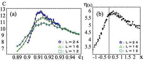
Figure 1: (a) System-size dependence of specific heat $C$ for $N=2$ at $c_{2}=0.4$. (b) Scaling function $\eta(x)$ for Fig.1(a).

The above results for $N=2$ are consistent with the “prediction” given above. The sum $\tilde{\varphi}_{x+}\equiv\varphi_{x1}+\varphi_{x2}$ couples with the compact gauge field and generates no phase transitionjanke , while the difference $\tilde{\varphi}_{x-}\equiv\varphi_{x1}-\varphi_{x2}$ behaves like the angle variable in the 3D $XY$ model. The 3D $XY$ model has a second-order phase transition with the critical exponent $\nu=0.666...$XY . Our value of $\nu$ obtained above is very close to this value. However, it should be remarked that the simple separation of variables in terms of $\tilde{\varphi}_{\pm}$ is not perfect due to the higher-order terms in the compact gauge theory. Nonetheless, our numerical studies strongly suggests that the phase transition for $N=2$ belongs to the universality class of the 3D $XY$ model.

It is instructive to see the behavior of the instanton density $\rho$. We employ the definition of $\rho$ in the 3D U(1) compact lattice gauge theory given by DeGrand and Toussaintinstanton . $\rho$ in Fig.2 decreases very rapidly near the phase transition point. This indicates that a “crossover” from dense to dilute instanton “phases” occurs simultaneously with the phase transition. In other words, the observed phase transition can be interpreted as a confinement(small $c_{1}$)-Higgs(large $c_{1}$) phase transition.

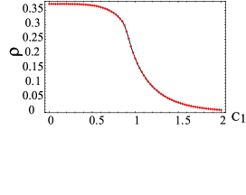
Figure 2: Instanton density $\rho$ for $N=2$ at $c_{2}=0.4$ as a function of $c_{1}$.

In Fig.3, we present the phase diagram for $N=2$ in the $c_{2}$-$c_{1}$ plane. There exists a second-order phase transition line separating the confinement and the Higgs phases. There also exists a crossover line similar to that in the 3D $N=1$ U(1) Higgs modeljanke .

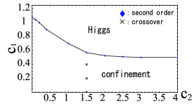
Figure 3: Phase diagram for $N=2$. There are two phases, confinement and Higgs, separated by second-order phase transition line. There also exists a crossover line in the confinement phase separating dense and dilute instanton-density regions.

Let us turn to the $N=3$ case. Among many possibilities of three $c_{1a}$’s, we first consider the symmetric case $c_{11}=c_{12}=c_{13}\equiv c_{1}$. One may expect that there are two ($N-1=2$) second-order transitions that may coincide at a certain critical point. Studying the $N=3$ case is interesting from a general viewpoint of the critical phenomena, i.e., whether coincidence of multiple phase transitions changes the order of the transition. We studied various points in the $c_{2}-c_{1}$ plane and found that the order of transition changes as $c_{2}$ varies. In Fig.4, we show $E$ and $\rho$ along $c_{2}=1.5$ as a function of $c_{1}$. Both quantities show hysteresis loops, which are signals of a first-order phase transition. In Fig.5, we present $C$ at $c_{2}=3.0$. The peak of $C$ at around $c_{1}\sim 0.48$ develops as $L$ is increased, whereas $E$ shows no discontinuity and hysteresis. Therefore, we conclude that the phase transition at $(c_{2},c_{1})\sim(3.0,0.48)$ is second order. In Fig.6(a), we present the phase diagram of the symmetric case for $N=3$, where the order of transition between the confinement and Higgs phases changes from first (smaller $c_{2}$) to second order (larger $c_{2}$). In Fig.6(b) we present $C$ along $c_{1}=0.2$, which shows a smooth nondeveloping peak. $\rho$ decreases smoothly around this peak. These results indicate crossovers at $c_{2}\simeq 1.5$.

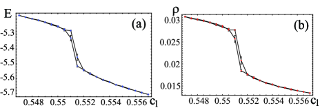
Figure 4: (a) Internal energy $E$ and (b) instanton density $\rho$ for $N=3$ at $c_{2}=1.5$ and $L=16$. Both exhibit hysteresis loops indicating a first-order phase transition at $c_{1}\simeq 0.551$.

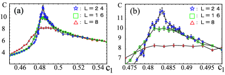
Figure 5: (a) Specific heat for $N=3$ at $c_{2}=3.0$. (b) Close-up view near the peak. The peak develops as $L$ increases.

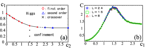
Figure 6: (a) Phase diagram for the $N=3$ symmetric case. The phase transitions are first order in the region $c_{2}\lesssim 2.25$, whereas they are second order in the region $c_{2}\gtrsim 2.25$. There exists a tricritical point at around $(c_{2},c_{1})\sim(2.25,0.5)$. Crosses near $c_{2}=1.5$ line show crossovers. (b) Specific heat for $N=3$ at $c_{1}=0.2$. It has a system-size independent smooth peak at which a crossover takes place.

Then it becomes interesting to consider asymmetric cases, e.g., $c_{11}\neq c_{12}=c_{13}$. This case is closely related to a doped AF magnet. $\phi_{2}$ and $\phi_{3}$ correspond there to the $CP^{1}$ spinon field in the deep easy-plane limit, whereas $\phi_{1}$ corresponds to doped holes. This case is also relevant to cosmology because the order of Higgs phase transition in the early universe is important in the inflational cosmology. Furthermore, one may naively expect that once a phase transition to the Higgs phase occurs at certain temperature $T$, no further phase transitions take place at lower $T$’s even if the gauge field couples with other Higgs bosons. However, our investigation below will show that this is not the case.

Let us consider the case $c_{12}=c_{13}=2c_{11}$, which we call the $c_{1}=(1,2,2)$ model, and focus on the case $c_{2}=1.0$. As shown in Fig.7(a), $C$ exhibits two peaks at $c_{11}\sim 0.35$ and $0.52$. Figs.7(b),(c) present the detailed behavior of $C$ near these peaks, which show that the both peaks develop as $L$ is increased. We conclude that both of these peaks show second-order transitions. This result is interpreted as the first-order phase transition in the symmetric $N=3$ model is decomposed into two second-order transitions in the $c_{1}=(1,2,2)$ model.

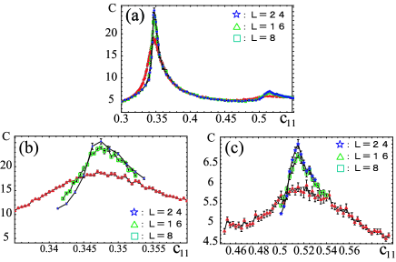
Figure 7: (a) Specific heat of the $c_{1}=(1,2,2)$ model ($N$=3) at $c_{2}=1.0$. (b,c) Close-up views of $C$ near (b) $c_{11}\sim 0.35$ and (c) $c_{11}\sim 0.52$.

Let us turn to the opposite case, $c_{12}=c_{13}=0.5c_{11}$, i.e., the $c_{1}=(2,1,1)$ model at $c_{2}=1.0$. One may expect that two second-order phase transitions appear as in the previous $c_{1}=(1,2,2)$ model. However, the result shown in Fig.8 indicates that there exists only one second-order phase transition near $c_{11}\sim 1.08$. The broad and smooth peak near $c_{11}\sim 0.85$ shows no $L$ dependence and we conclude that it is a crossover. This crossover is similar to that in the ordinary $N=1$ gauge-Higgs system as we shall see by the measurement of $\rho$ below.

The orders of these transitions are understood as follows: In the $c_{1}=(1,2,2)$ model, as we increase $c_{11}$, the two modes $\phi_{xa}(a=2,3)$ with larger $c_{1a}$ firstly become relevant and the model is effectively the symmetric $N=2$ model. The peak in Fig.7(b) is interpreted as the second-order peak of this model. For higher $c_{11}$’s, the gauge field is negligible due to small fluctuations, and the effective model is the $N=1$ $XY$ model of $\phi_{x1}$. It gives the second-order peak in Fig.7(c). Similarly, in the $c_{1}=(2,1,1)$ model, $\phi_{x1}$ firstly becomes relevant. The effective model is the $N=1$ model, which gives the broad peak in Fig.8 as the crossoverjanke . For higher $c_{11}$’s, the effective model is the $N=2$ symmetric model of $\phi_{x2},\phi_{x3}$ and $U_{x\mu}$, giving the sharp second-order peak in Fig.8.

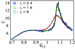
Figure 8: Specific heat of the $c_{1}=(2,1,1)$ model at $c_{2}=1.0$.

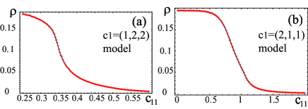
Figure 9: Instanton density $\rho$ at $c_{2}=1.0$ in the (a) $c_{1}=(1,2,2)$ model and (b) $c_{1}=(2,1,1)$ model.

In Fig.9, we present $\rho$ of the $c_{1}=(1,2,2)$ and $(2,1,1)$ models as a function of $c_{11}$. $\rho$ of the $c_{1}=(1,2,2)$ model decreases very rapidly at around $c_{11}\sim 0.35$, which is the phase transition point in lower $c_{11}$ region. On the other hand, at the higher phase transition point, $c_{11}\sim 0.52$, $\rho$ shows no significant changes. This observation indicates that the lower-$c_{11}$ phase transition is the confinement-Higgs transition, whereas the higher-$c_{11}$ transition is a charge-neutral $XY$-type phase transition.

On the other hand, $\rho$ of the $c_{1}=(2,1,1)$ model decreases rapidly at around $c_{11}\sim 0.85$, where $C$ exhibits a broad peak. This indicates that the crossover from the dense to dilute-instanton regions occurs there just like in the $N=1$ casejanke . No “anomalous” behavior of $\rho$ is observed at the critical point $c_{11}\sim 1.1$, and therefore the phase transition is that of the neutral mode.

We have also studied the symmetric case for $N=4,5$ at $c_{2}=0$. Both cases show clear signals of first-order transitions at $c_{1}\simeq 0.89(N=4),0.86(N=5)$. On the other hand, at $c_{2}=\infty$, the gauge dynamics is “frozen” to $U_{x\mu}=1$ up to gauge transformations, so there remain $N$-fold independent $XY$ spin models, which show a second-order transition at $c_{1}\simeq 0.46$. Thus we expect a tricritical point for general $N>2$ at some finite $c_{2}$ separating first-order and second-order transitions.

Let us summarize the results. For $N=2$ there is a critical line $\tilde{c}_{1}(c_{2})$ of second-order transitions in the $c_{2}-c_{1}$ plane, which distinguishes the Higgs phase ($c_{1}>\tilde{c}_{1}$) and the confinement phase ($c_{1}<\tilde{c}_{1}$). This result is consistent with Kragset et al.kragset . For $N=3$ there is a similar transition line, but the region $0<c_{2}<c_{2c}\simeq 2.25$ is of second-order transitions while the region $c_{2c}<c_{2}$ is of first-order transitions. To study the mechanism of generation of these first-order transitions, we studied the asymmetric cases and found two second-order transitions [in the $c_{1}=(1,2,2)$ model] or one crossover and one second-order phase transition [in the $c_{1}=(2,1,1)$ model]. The former case implies that two simultaneous second-order transitions strengthen the order to generate a first-order transition. Chernodub et al.chernodub reported a similar generation of an enhanced first-order transition in a related 3D Higgs model with singly and doubly charged scalar fields. We stress that the above change of the order is dynamical because (1) It depends on the value of $c_{2}$, (2) Related 3D models, the $CP^{N-1}$ and $N$-fold $CP^{1}$ gauge models, exhibit always second-order transitions (See the last reference of Ref.gauge ).

We thank Dr.K. Sakakibara for useful discussion.

References

- (1) See, e.g., S. Coleman, “Aspects of Symmetry” (Cambridge University Press 1985).
- (2) Y. Iwasaki, K. Kanaya, S. Sakai, and T. Yoshie, Phys. Rev. Lett.69, 21 (1992); G. Arakawa, I. Ichinose, T. Matsui, K. Sakakibara, Phys. Rev. Lett.94, 211601 (2005); S. Takashima, I. Ichinose, T. Matsui, Phys. Rev. B73, 075119 (2006).
- (3) E. Babaev, A. Sudbø, and N. W. Ashcroft, Nature 431, 666 (2004).
- (4) Y. Ohashi, Phys. Rev. Lett. 94, 050403 (2005).
- (5) T. Senthil, L. Balents, S. Sachdev, A. Vishwanath, and M. P. A. Fisher, Science 303, 1490 (2004); T. Senthil, A. Vishwanath, L. Balents, S. Sachdev, and M. P. A. Fisher, Phys. Rev. B70, 144407 (2004).
- (6) Similar limit may be taken to relate the superconductivity of ultracold fermionic atoms with spin to the U(1) gauge model with Higgs fields. J. Zhao, K. Ueda, and X. Wang, Phys. Rev. B74, 233102 (2006), considered the Hubbard model to describe the superconductivity of fermionic atoms, which has a -component order parameter. At large repulsion and at the filling factor , the model becomes the U(1) gauge model with spins. A variable is parametrized as with . In the symmetric limit, which is the easy-plane limit for , and becomes a Higgs field.
- (7) R. K. Kaul, A. Kolezhuk, M. Levin, S. Sachdev, and T. Senthil, arXiv:cond-mat/0611536.
- (8) A. B. Kukulov, N. V. Prokof’ev, B. V. Svistunov, and M. Troyer, Ann. Phys. 321, 1602 (2006).
- (9) A. H. Guth, Phys. Rev. D23,347 (1981).
- (10) R. Allahverdi, K. Enqvist, J. Carcia-Bellido, and A. Mazumdar, arXiv:hep-ph/0605035.
-
(11)
S. Wenzel, E. Bittner, W. Janke, A.M.J. Schakel, and
A. Schiller, Phys. Rev. Lett. 95, 051601(2005). - (12) J. Smiseth, E. Smørgrav, and A. Sudbø, Phys. Rev. Lett. 93, 077002 (2004).
- (13) S. Kragset, E. Smørgrav, J. Hove, F. S. Nogueira, and A. Sudbø, Phys. Rev. Lett. 97, 247201 (2006).
- (14) M. Campostrini, M. Hasenbusch, A. Pelissetto, P. Rossi, and E. Vicari, Phys. Rev. B63, 214503 (2001).
- (15) T. A. DeGrand and D. Toussaint, Phys. Rev. D22, 2478 (1980).
- (16) M. N. Chernodub, E.-M. Ilgenfritz, and A.Schller, Phys. Rev. B73, 100506 (2006).