Antenna Combining for the MIMO Downlink Channel

Abstract

A multiple antenna downlink channel where limited channel feedback is available to the transmitter is considered. In a vector downlink channel (single antenna at each receiver), the transmit antenna array can be used to transmit separate data streams to multiple receivers only if the transmitter has very accurate channel knowledge, i.e., if there is high-rate channel feedback from each receiver. In this work it is shown that channel feedback requirements can be significantly reduced if each receiver has a small number of antennas and appropriately combines its antenna outputs. A combining method that minimizes channel quantization error at each receiver, and thereby minimizes multi-user interference, is proposed and analyzed. This technique is shown to outperform traditional techniques such as maximum-ratio combining because minimization of interference power is more critical than maximization of signal power in the multiple antenna downlink. Analysis is provided to quantify the feedback savings, and the technique is seen to work well with user selection and is also robust to receiver estimation error.

I Introduction

Multi-user MIMO techniques such as zero-forcing beamforming allow for simultaneous transmission of multiple data streams even when each receiver (mobile) has only a single antenna, but very accurate channel state information (CSI) is generally required at the transmitter in order to utilize such techniques. In the practically motivated finite rate feedback model, each mobile feeds back a finite number of bits describing its channel realization at the beginning of each block or frame. In the vector downlink channel (multiple transmit antennas, single antenna at each receiver), the feedback bits are determined by quantizing the channel vector to one of $2^{B}$ quantization vectors. While a relatively small number of feedback bits suffice to obtain near-perfect CSIT performance in a point-to-point vector/MISO (multiple-input, single-output) channel [1], considerably more feedback is required in a vector downlink channel. If zero-forcing beamforming (ZFBF) is used, the feedback rate must be scaled with the number of transmit antennas as well as SNR in order to achieve rates close to perfect CSIT systems [2]. In such a system the transmitter emits multiple beams and uses its channel knowledge to select beamforming vectors such that nulls are created at certain users. Inaccurate CSI leads to inaccurate nulling and thus translates directly into multi-user interference and reduced SINR/throughput.

In this paper we consider the MIMO downlink channel, in which the transmitter and each mobile have multiple antennas ($M$ transmit antennas, $N$ antennas per mobile), in the same limited feedback setting. We propose a receive antenna combining technique, dubbed quantization-based combining (QBC), that converts the MIMO downlink into a vector downlink in such a way that the system is able to operate with reduced channel feedback. Each mobile linearly combines its $N$ antenna outputs and thereby creates a single antenna channel. The resulting vector channel is quantized and fed back, and transmission is then performed as in a normal vector downlink channel.

With QBC the combiner weights are chosen on the basis of both the channel and the vector quantization codebook to produce the effective single antenna channel that can be quantized most accurately. On the other hand, traditional combining techniques such as the maximum-ratio based technique that is optimal for point-to-point MIMO channels with limited channel feedback [3] or direct quantization of the maximum eigenmode are aimed towards maximization of received signal power but generally do not minimize channel quantization error. Since channel quantization error is so critical in the MIMO downlink channel, quantization-based combining leads to better performance by minimizing quantization error (i.e., interference power) possibly at the expense of channel (i.e., signal) power.

One way to view the advantage of QBC is through its reduced feedback requirements relative to the vector downlink channel. In [2] it is shown that scaling (per mobile) feedback as $B=\frac{M-1}{3}P_{dB}$, where $P$ represents the SNR, suffices to maintain a maximum gap of 3 dB (equivalent to 1 bps/Hz per mobile) between perfect CSIT and limited feedback performance in a vector downlink channel employing ZFBF. With QBC, our analysis shows that the same throughput (3 dB away from a vector downlink with perfect CSIT) can be achieved if feedback is scaled at the slower rate of $B\approx\frac{M-N}{3}P_{dB}$. In other words, QBC allows a MIMO downlink to mimic vector downlink performance with reduced channel feedback.

Alternatively, QBC can be thought of as an effective method to utilize multiple receive antennas in a downlink channel in the presence of limited channel feedback. Although it is possible to send multiple streams to each mobile if receive combining is not performed, this requires even more feedback from each mobile than a single-stream approach. In addition, QBC has the advantage that the transmitter need not be aware of the number of receive antennas being used.

The remainder of this paper is organized as follows: In Section II we introduce the system model and some preliminaries. In Section III we describe a simple antenna selection method that leads directly into Section IV where the much more powerful quantization-based combining technique is described in detail. In Section V we analyze the throughput and feedback requirements of QBC. In Section VI we compare QBC to alternative MIMO downlink techniques, and finally we conclude in Section VII.

II System Model and Preliminaries

We consider a $K$ mobile (receiver) downlink channel in which the transmitter (access point) has $M$ antennas, and each of the mobiles has $N$ antennas. The received signal at the $i$-th antenna is given by:

$$y_{i}={\mathbf{h}}_{i}^{H}{\mathbf{x}}+n_{i},~{}~{}~{}i=1,\ldots,NK$$ (1)

where ${\bf h}_{1},{\bf h}_{2},\ldots,{\bf h}_{KN}$ are the channel vectors (with ${\bf h}_{i}\in{\mathbb{C}}^{M\times 1}$) describing the $KN$ receive antennas, ${\bf x}\in{\mathbb{C}}^{M\times 1}$ is the transmitted vector, and ${\bf n}_{1},\ldots,{\mathbf{n}}_{NK}$ are independent complex Gaussian noise terms with unit variance. The $k$-th mobile has access to $y_{(k-1)N+1},\ldots,y_{Nk}$. The input must satisfy a power constraint of $P$, i.e. $E[||{\mathbf{x}}||^{2}]\leq P$. We use ${\bf H}_{k}$ to denote the concatenation of the $k$-th mobile’s channels, i.e. ${\bf H}_{k}=[{\bf h}_{(k-1)N+1}\cdots{\bf h}_{Nk}]$. We consider a block fading channel with iid Rayleigh fading from block to block, i.e., the channel coefficients are iid complex Gaussian with unit variance. Each of the mobiles is assumed to have perfect knowledge of its own channel ${\bf H}_{i}$, although we analyze the effect of relaxing this assumption in Section V-C. In this work we study only the ergodic capacity, or the long-term average throughput. Furthermore, we only consider systems for which $N<M$ because QBC is not very useful if $N\geq M$; this point is briefly discussed in Section IV.

II-A Finite Rate Feedback Model

In the finite rate feedback model, each mobile quantizes its channel to $B$ bits and feeds back the bits perfectly and instantaneously to the transmitter at the beginning of each block [3][4]. Vector quantization is performed using a codebook ${\mathcal{C}}$ of $2^{B}$ $M$-dimensional unit norm vectors ${\mathcal{C}}\triangleq\{\mathbf{w}_{1},\ldots,\mathbf{w}_{2^{B}}\}$, and each mobile quantizes its channel to the quantization vector that forms the minimum angle to it [3] [4]:

$$\hat{{\bf h}}_{k} = \textrm{arg}\min_{{\bf w}={\bf w}_{1},\ldots,{\bf w}_{2^{B}}}\sin^{2}\left(\angle({\bf h}_{k},{\bf w})\right).$$ (2)

For analytical tractability, we study systems using random vector quantization (RVQ) in which each of the $2^{B}$ quantization vectors is independently chosen from the isotropic distribution on the $M$-dimensional unit sphere and where each mobile uses an independently generated codebook [5]. We analyze performance averaged over random codebooks; similar to Shannon’s random coding argument, there always exists at least one quantization codebook that performs as well as the ensemble average.

II-B Zero-Forcing Beamforming

After receiving the quantization indices from each of the mobiles, the AP can use zero-forcing beamforming (ZFBF) to transmit data to up to $M$ users. For simplicity let us consider the $N=1$ scenario, where the channels are the vectors ${\bf h}_{1},\ldots,{\bf h}_{M}$. When ZFBF is used, the transmitted signal is defined as ${\bf x}=\sum_{k=1}^{M}x_{k}{\bf v}_{k}$, where each $x_{k}$ is a scalar (chosen complex Gaussian) intended for the $k$-th mobile, and ${\bf v}_{k}\in{\mathcal{C}}^{M}$ is the $k$-th mobile’s BF vector. If there are $M$ mobiles (randomly selected), the beamforming vectors ${\bf v}_{1},\ldots,{\bf v}_{M}$ are chosen as the normalized rows of the matrix $[\hat{{\bf h}}_{1}\cdots\hat{{\bf h}}_{M}]^{-1}$, i.e., they satisfy $||{\bf v}_{k}||=1$ for all $k$ and $\hat{{\bf h}}_{k}^{H}{\bf v}_{j}=0$ for all $j\neq k$. If all multi-user interference is treated as additional noise and equal power loading is used, the resulting SINR at the $k$-th receiver is given by:

$$SINR_{k}=\frac{\frac{P}{M}|{\bf h}_{k}^{H}{\bf v}_{k}|^{2}}{1+\sum_{j\neq k}\frac{P}{M}|{\bf h}_{k}^{H}{\bf v}_{j}|^{2}}.$$ (3)

The coefficient that determines the amount of interference received at mobile $k$ from the beam intended for mobile $j$, $|{\bf h}_{k}^{H}{\bf v}_{j}|^{2}$, is easily seen to be an increasing function of mobile $k$’s quantization error.

In the above expression we have assumed that $M$ mobiles are randomly selected for transmission and that equal power is allocated to each mobile. However, the throughput of zero-forcing based MIMO downlink channels can be significantly increased by transmitting to an intelligently selected subset of mobiles [6]. In order to maximize throughput, users with nearly orthogonal channels and with large channel magnitudes are selected, and waterfilling can be performed across the channels of the selected users. In [7] a low-complexity greedy algorithm that selects users and performs waterfilling is proposed. If this algorithm is used, a zero-forcing based system can come quite close to the true sum capacity of the MIMO downlink, even for a moderate number of users.

II-C MIMO Downlink with Single Antenna Mobiles

In [2] the vector downlink channel ($N=1$) is analyzed assuming that equal power ZFBF is performed without user selection on the basis of finite rate feedback (with RVQ). The basic result of [2] is that:

$$R_{FB}(P)\geq R_{CSIT}(P)-\log_{2}\left(1+P\cdot E\left[\sin^{2}\left(\angle(\hat{{\bf h}_{k}},{\bf h}_{k})\right)\right]\right)$$ (4)

where $R_{FB}(P)$ and $R_{CSIT}(P)$ are the ergodic per-user throughput with feedback and with perfect CSIT, respectively, and the quantity $E\left[\sin^{2}\left(\angle(\hat{{\bf h}_{k}},{\bf h}_{k})\right)\right]$ is the expected quantization error. The expected quantization error can be accurately upper bounded by $2^{-\frac{B}{M-1}}$ and therefore the throughput loss due to limited feedback is upper bounded by $\log_{2}\left(1+P\cdot 2^{-\frac{B}{M-1}}\right)$, which is an increasing function of the SNR $P$. If the number of feedback bits (per mobile) is scaled with $P$ according to:

$$B=(M-1)\log_{2}P\approx\frac{M-1}{3}P_{dB},$$

then the difference between $R_{FB}(P)$ and $R_{CSIT}(P)$ is upper bounded by $1$ bps/Hz at all SNR’s, or equivalently the power gap is at most 3 dB. As the remainder of the paper shows, quantization-based combining significantly reduces the quantization error (more precisely, it increases the exponential rate at which quantization error goes to zero as $B$ is increased) and therefore decreases the rate at which $B$ must be increased as a function of SNR.

III Antenna Selection for Reduced Quantization Error

In this section we describe a simple antenna selection method that reduces channel quantization error. Description of this technique is primarily included for expository reasons, because the simple concept of antenna selection naturally extends to the more complex (and powerful) QBC technique. In point-to-point MIMO, antenna selection corresponds to choosing the receive antenna with the largest channel gain, while in the MIMO downlink the receive antenna that can be vector quantized with minimal angular error is selected. Mobile 1, which has channel matrix ${\bf H}_{1}=[{\bf h}_{1}\cdots{\bf h}_{N}]$ and a single quantization codebook consisting of $2^{B}$ quantization vectors ${\bf w}_{1},\ldots,{\bf w}_{2^{B}}$, first individually quantizes each of its $N$ vector channels ${\bf h}_{1},\ldots,{\bf h}_{N}$

$$\hat{\bf g}_{i} = \textrm{arg}\min_{{\bf w}={\bf w}_{1},\ldots,{\bf w}_{2^{B}}}\sin^{2}\left(\angle({\bf h}_{i},{\bf w})\right)~{}~{}~{}~{}i=1,\ldots,N,$$ (5)

and then selects the antenna with the minimum quantization error:

$$j=\textrm{arg}\min_{i=1,\ldots,N}\sin^{2}\left(\angle({\bf h}_{i},\hat{{\bf g}_{i}})\right),$$ (6)

and feeds back the quantization index corresponding to $\hat{{\bf g}_{j}}$. The mobile uses only antenna $j$ for reception, and thus the system is effectively transformed into a vector downlink channel.

Due to the independence of the channel and quantization vectors, choosing the best of $N$ channel quantizations is statistically equivalent to quantizing a single vector channel using a codebook of size $N\cdot 2^{B}$. Therefore, antenna selection effectively increases the quantization codebook size from $2^{B}$ to $N\cdot 2^{B}$, and thus the system achieves the same throughput as a vector downlink with $B+\log_{2}N$ feedback bits. Although not negligible, this advantage is much smaller than that provided by quantization-based combining.

IV Quantization-Based Combining

In this section we describe the quantization-based combining (QBC) technique that reduces channel quantization error by appropriately combining receive antenna outputs. We consider a linear combiner at each mobile, which effectively converts each multiple antenna mobile into a single antenna receiver. The combiner structure for a 3 user channel with 3 transmit antennas ($M=3$) and 2 antennas per mobile ($N=2$) is shown in Fig. 1. Each mobile linearly combines its $N$ outputs, using appropriately chosen combiner weights, to produce a scalar output (denoted by $y^{\textrm{eff}}_{k}$). The effective channel describing the channel from the transmit antenna array to the effective output of the $k$-th mobile ($y^{\textrm{eff}}_{k}$) is simply a linear combination of the $N$ vectors describing the $N$ receive antennas. After choosing combining weights the mobile quantizes the effective channel vector and feeds back the appropriate quantization index. Only the effective channel output is used to receive data, and thus each mobile effectively has only one antenna.

The key to the technique is to choose combiner weights that produce an effective channel that can be quantized very accurately; such a choice must be made on the basis of both the channel vectors and the quantization codebook. This is quite different from maximum ratio combining, where the combiner weights and quantization vector are chosen such that received signal power is maximized but quantization error is generally not minimized. Note that antenna selection corresponds to choosing the effective channel from the $N$ columns of ${\bf H}_{k}$, while QBC allows for any linear combination of these $N$ column vectors.

Figure 1: Effective Channel for $M=K=3$, $N=2$ System

IV-A General Description

Let us consider the effective received signal at the first mobile for some choice of combiner weights, which we denote as $\boldsymbol{\gamma}_{1}=(\gamma_{1,1},\ldots,\gamma_{1,N})$. In order to maintain a noise variance of one, the combiner weights are constrained to have unit norm: $||\boldsymbol{\gamma}_{1}||=1$. The (scalar) combiner output, denoted $y^{\textrm{eff}}_{1}$, is:

$$y^{\textrm{eff}}_{1}=\sum_{i=1}^{N}\gamma_{1,i}^{H}({\bf h}_{i}^{H}{\bf x}+n_{i}) = \left(\sum_{i=1}^{N}\gamma_{1,i}^{H}{\bf h}_{i}^{H}\right){\bf x}+\sum_{i=1}^{N}\gamma_{1,i}^{H}n_{k}$$

$$= ({\bf h}^{\textrm{eff}}_{1})^{H}{\bf x}+n,$$

where $n=\sum_{i=1}^{N}\gamma_{1,i}^{H}n_{i}$ is unit variance complex Gaussian because $|\boldsymbol{\gamma}_{1}|=1$. The effective channel vector ${\bf h}^{\textrm{eff}}_{1}$ is simply a linear combination of the vectors ${\bf h}_{1},\ldots,{\bf h}_{N}$: ${\bf h}^{\textrm{eff}}_{1}=\sum_{i=1}^{N}\gamma_{1,i}{\bf h}_{i}={\bf H}_{1}{\boldsymbol{\gamma}}_{1}$. Since $\boldsymbol{\gamma}_{1}$ can be any unit norm vector, ${\bf h}^{\textrm{eff}}_{1}$ can be in any direction in the $N$-dimensional subspace spanned by ${\bf h}_{1},\ldots,{\bf h}_{N}$, i.e., in span$({\bf H}_{1})$.

Because quantization error is so critical to performance, the objective is to choose combiner weights that yield an effective channel that can be quantized with minimal error. The error corresponding to effective channel ${\bf h}^{\textrm{eff}}_{1}$ is

$$\min_{l=1,\ldots,2^{B}}\sin^{2}\left(\angle({\bf h}^{\textrm{eff}}_{1},{\bf w}_{l})\right).$$ (7)

Therefore, the optimal choice of the effective channel is the solution to:

$$\min_{{\bf h}^{\textrm{eff}}_{1}}~{}~{}\min_{l=1,\ldots,2^{B}}\sin^{2}\left(\angle({\bf h}^{\textrm{eff}}_{1},{\bf w}_{l})\right),$$ (8)

where ${\bf h}^{\textrm{eff}}_{1}$ is allowed to be in any direction in span$({\bf H}_{1})$. Once the optimal effective channel is determined, the combiner weights $\boldsymbol{\gamma}_{1}$ can be determined through a simple pseudo-inverse operation.

Since the expression for the optimum effective channel given in (8) consists of two minimizations, without loss of optimality the order of the minimization can be switched to give:

$$\min_{l=1,\ldots,2^{B}}~{}\min_{{\bf h}^{\textrm{eff}}_{1}}~{}~{}\sin^{2}\left(\angle({\bf h}^{\textrm{eff}}_{1},{\bf w}_{l})\right),$$ (9)

For each quantization vector ${\bf w}_{l}$, the inner minimization finds the effective channel vector in span$({\bf H}_{1})$ that forms the minimum angle with ${\bf w}_{l}$. By basic geometric principles, the minimizing ${\bf h}^{\textrm{eff}}_{1}$ is the projection of ${\bf w}_{l}$ on span$({\bf H}_{1})$. The solution to the inner minimization in (9) is therefore the sine squared of the angle between ${\bf w}_{l}$ and its projection on span$({\bf H}_{1})$, which is referred to as the angle between ${\bf w}_{l}$ and the subspace. As a result, the best quantization vector, i.e., the solution of (9), is the vector that forms the smallest angle between itself and span$({\bf H}_{1})$. The optimal effective channel is the (scaled) projection of this particular quantization vector onto span$({\bf H}_{1})$.

In order to perform quantization, the angle between each quantization vector and span$({\bf H}_{1})$ must be computed. If ${\bf q}_{1},\ldots,{\bf q}_{N}$ form an orthonormal basis for span$({\bf H}_{1})$ and ${\bf Q}_{1}\triangleq[{\bf q}_{1}\cdots{\bf q}_{N}]$, then $\sin^{2}(\angle({\bf w},\textrm{span}({\bf H}_{1})))=1-||{\bf Q}_{1}^{H}{\bf w}||^{2}$. Therefore, mobile 1’s quantized channel, denoted $\hat{{\bf h}_{1}}$, is:

$$\hat{{\bf h}}_{1}=\textrm{arg}\min_{{\bf w}={\bf w}_{1},\ldots,{\bf w}_{2^{B}}}|\angle({\bf w},\textrm{span}({\bf H}_{1}))| = \textrm{arg}\max_{{\bf w}={\bf w}_{1},\ldots,{\bf w}_{2^{B}}}||{\bf Q}_{1}^{H}{\bf w}||^{2}.$$ (10)

Once the quantization vector has been selected, it only remains to choose the combiner weights. The projection of $\hat{{\bf h}}_{1}$ on span$({\bf H}_{1})$, which is equal to ${\bf Q}_{1}{\bf Q}_{1}^{H}\hat{{\bf h}}_{1}$, is scaled by its norm to produce the unit norm vector ${\bf s}_{1}^{\textrm{proj}}$. The direction specified by ${\bf s}_{1}^{\textrm{proj}}$ has the minimum quantization error amongst all directions in span$({\bf H}_{1})$, and therefore the effective channel should be chosen in this direction. First we find the vector $\bf{u}_{1}\in\mathcal{C}^{N}$ such that ${\bf H}_{1}{\bf u}_{1}={\bf s}_{1}^{\textrm{proj}}$, and then scale to get ${\boldsymbol{\gamma}}_{1}$. Since ${\bf s}_{1}^{\textrm{proj}}$ is in span$({\bf H}_{1})$, ${\bf u}_{1}$ is uniquely determined by the pseudo-inverse of ${\bf H}_{1}$:

$${\bf u}_{1}=\left({\bf H}_{1}^{H}{\bf H}_{1}\right)^{-1}{\bf H}_{1}^{H}{\bf s}_{1}^{\textrm{proj}},$$ (11)

and the combiner weight vector ${\boldsymbol{\gamma}}_{1}$ is the normalized version of ${\bf u}_{1}$: $\boldsymbol{\gamma}=\frac{{\bf u}_{1}}{||{\bf u}_{1}||}$. The quantization procedure is illustrated for a $N=2$ channel in Fig. 2. In the figure the span of the two channel vectors is shown along with the quantization vector ${\bf h}_{1}$, its projection on the channel subspace, and the effective channel.

IV-B Algorithm Summary

We now summarize the quantization-based combining procedure performed at the $k$-th mobile:

1. Find an orthonormal basis, denoted ${\bf q}_{1},\ldots,{\bf q}_{N}$, for span(${\bf H}_{k}$) and define ${\bf Q}_{k}\triangleq[{\bf q}_{1}\cdots{\bf q}_{N}]$.

2. Find the quantization vector closest to the channel subspace:

   $$\hat{{\bf h}}_{k} = \textrm{arg}\max_{{\bf w}={\bf w}_{1},\ldots,{\bf w}_{2^{B}}}||{\bf Q}_{k}^{H}{\bf w}||^{2}.$$ (12)

3. Determine the direction of the effective channel by projecting $\hat{{\bf h}_{k}}$ onto span(${\bf H}_{k}$).

   $${\bf s}_{k}^{\textrm{proj}}=\frac{{\bf Q}_{k}{\bf Q}_{k}^{H}\hat{{\bf h}_{k}}}{||{\bf Q}_{k}{\bf Q}_{k}^{H}\hat{{\bf h}_{k}}||}.$$ (13)

4. Compute the combiner weight vector ${\boldsymbol{\gamma}}_{k}$:

   $${\boldsymbol{\gamma}}_{k}=\frac{\left({\bf H}_{k}^{H}{\bf H}_{k}\right)^{-1}{\bf H}_{k}^{H}{\bf s}_{1}^{\textrm{proj}}}{||\left({\bf H}_{k}^{H}{\bf H}_{k}\right)^{-1}{\bf H}_{k}^{H}{\bf s}_{1}^{\textrm{proj}}||}.$$ (14)

Each mobile performs these steps, feeds back the index of its quantized channel $\hat{{\bf h}_{k}}$, and then linearly combines its $N$ received signals using vector ${\boldsymbol{\gamma}}_{k}$ to produce its effective channel output $y^{\textrm{eff}}_{k}=({\bf h}^{\textrm{eff}}_{k})^{H}{\bf x}+n$ with ${\bf h}^{\textrm{eff}}_{k}={\bf H}_{k}{\boldsymbol{\gamma}}_{k}$. Note that the transmitter need not be aware of the number of receive antennas or of the details of this procedure because the downlink channel appears to be a single receive antenna channel from the transmitter’s perspective; this clearly eases the implementation burden of QBC.

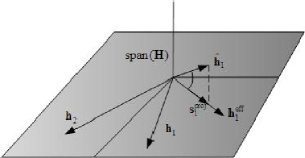
Figure 2: Quantization procedure for a two antenna mobile

V Throughput Analysis

Quantization-based combining converts the MIMO downlink channel into a vector downlink with channel vectors ${\bf h}^{\textrm{eff}}_{1},\ldots,{\bf h}^{\textrm{eff}}_{K}$ and channel quantizations $\hat{{\bf h}}_{i}\cdots\hat{{\bf h}}_{K}$. We first derive the statistics of the effective vector channel, then analyze throughput for ZFBF with equal power loading and no user selection, and finally quantify the effect of receiver estimation error.

V-A Channel Statistics

We first determine the distribution of the quantization error and the effective channel vectors with respect to both the random channels and random quantization codebooks.

Lemma 1

The quantization error $\sin^{2}(\angle(\hat{{\bf h}_{k}},{\bf h}^{\textrm{eff}}_{k}))$, is the minimum of $2^{B}$ independent beta $(M-N,N)$ random variables.

Proof:

If the columns of $M\times N$ matrix ${\bf Q}_{k}$ form an orthonormal basis for span$({\bf H}_{k})$, then $\cos^{2}\left(\angle({\bf w}_{l},\textrm{span}({\bf H}_{k})\right)=||{\bf Q}_{k}^{H}{\bf w}_{l}||^{2}$ for any quantization vector. Since the basis vectors and quantization vectors are isotropically chosen and are independent, this quantity is the squared norm of the projection of a random unit norm vector in ${\mathcal{C}}^{M}$ onto a random $N$-dimensional subspace, which is described by the beta distribution with parameters $N$ and $M-N$ [9]. By the properties of the beta distribution, $\sin^{2}\left(\angle({\bf w}_{l},\textrm{span}({\bf H}_{k})\right)=1-\cos^{2}\left(\angle({\bf w}_{l},\textrm{span}({\bf H}_{k})\right)$ is beta $(M-N,N)$. Finally, the independence of the quantization and channel vectors implies independence of the $2^{B}$ random variables. ∎

Lemma 2

The normalized effective channels $\frac{{\bf h}^{\textrm{eff}}_{1}}{||{\bf h}^{\textrm{eff}}_{1}||},\ldots,\frac{{\bf h}^{\textrm{eff}}_{K}}{||{\bf h}^{\textrm{eff}}_{K}||}$ are iid isotropic vectors in ${\mathcal{C}}^{M}$.

Proof:

From the earlier description of QBC, note that $\frac{{\bf h}^{\textrm{eff}}_{k}}{||{\bf h}^{\textrm{eff}}_{k}||}={\bf s}_{k}^{\textrm{proj}}$, which is the projection of the best quantization vector onto span$({\bf H}_{k})$. Since each quantization vector is chosen isotropically, its projection is isotropically distributed within the subspace. Furthermore, the best quantization vector is chosen based solely on the angle between the quantization vector and its projection. Thus ${\bf s}_{k}^{\textrm{proj}}$ is isotropically distributed in span$({\bf H}_{k})$. Since this subspace is also isotropically distributed, the vector ${\bf s}_{k}^{\textrm{proj}}$ is isotropically distributed in ${\mathcal{C}}^{M}$. Finally, the independence of the quantization and channel vectors from mobile to mobile implies independence of the effective channel directions. ∎

Lemma 3

The quantity $||{\bf h}^{\textrm{eff}}_{k}||^{2}$ is $\chi^{2}_{2(M-N+1)}$.

Proof:

Using the notation from Section IV-A, the norm of the effective channel is given by:

$$||{\bf h}^{\textrm{eff}}_{k}||^{2}=||{\bf H}_{k}{\boldsymbol{\gamma}}_{k}||^{2}=||{\bf H}_{k}\frac{{\bf u}_{k}}{||{\bf u}_{k}||}||^{2}=\frac{1}{||{\bf u}_{k}||^{2}}||{\bf H}_{k}{\bf u}_{k}||^{2}=\frac{||{\bf s}_{k}^{\textrm{proj}}||^{2}}{||{\bf u}_{k}||^{2}}=\frac{1}{||{\bf u}_{k}||^{2}},$$ (15)

where we have used the definitions ${\bf h}^{\textrm{eff}}_{k}={\bf H}_{k}{\boldsymbol{\gamma}}_{k}$ and ${\boldsymbol{\gamma}}_{k}=\frac{{\bf u}_{k}}{||{\bf u}_{k}||}$, and the fact that ${\bf u}_{k}$ satisfies ${\bf H}_{k}{\bf u}_{k}={\bf s}_{k}^{\textrm{proj}}$. Therefore, in order to characterize the norm of the effective channel it is sufficient to characterize $\frac{1}{||{\bf u}_{k}||^{2}}$. The $N$-dimensional vector ${\bf u}_{k}$ is the set of coefficients that allows ${\bf s}_{k}^{\textrm{proj}}$, the normalized projection of the chosen quantization vector, to be expressed as a linear combination of the columns of ${\bf H}_{k}$ (i.e., the channel vectors). Because ${\bf s}_{k}^{\textrm{proj}}$ is isotropically distributed in span$({\bf H}_{k})$ (Lemma 2), if we change coordinates to any ($N$-dimensional) basis for span$({\bf H}_{k})$ we can assume without loss of generality that the projection of the quantization vector is $[1~{}0\cdots 0]^{T}$. Therefore, the distribution of $\frac{1}{||{\bf u}_{k}||^{2}}$ is the same as the distribution of $\frac{1}{\left[\left({\bf H}_{k}^{H}{\bf H}_{k}\right)^{-1}\right]_{1,1}}$. Since the $N\times N$ matrix ${\bf H}_{k}^{H}{\bf H}_{k}$ is Wishart distributed with $M$ degrees of freedom, this quantity is well-known to be $\chi^{2}_{2(M-N+1)}$; see [10] for a proof. ∎

The norm of the effective channel has the same distribution as that of a ($M-N+1$)-dimensional random vector instead of a $M$-dimensional vector. An arbitrary linear combination (with unit norm) of the $N$ channel vectors would result in another iid complex Gaussian $M$-dimensional vector, whose squared norm is $\chi^{2}_{2M}$, but the weights defining the effective channel are not arbitrary due to the inverse operation.

V-B Sum Rate Performance Relative to Perfect CSIT

After receiving the quantization indices from each of the mobiles, a simple transmission option is to perform equal-power ZFBF based on the channel quantizations (as described in Section II-B). If $K=M$ or $K>M$ and $M$ users are randomly selected, the resulting SINR at the $k$-th mobile is given by:

$$SINR_{k}=\frac{\frac{P}{M}|({\bf h}^{\textrm{eff}}_{k})^{H}{\bf v}_{k}|^{2}}{1+\sum_{j\neq k}\frac{P}{M}|({\bf h}^{\textrm{eff}}_{k})^{H}{\bf v}_{j}|^{2}}.$$ (16)

The ergodic sum rate achieved by QBC, denoted $R_{QBC}(P)$, is therefore given by:

$$R_{QBC}(P) = E_{{\bf H},\bf{W}}\left[\log_{2}\left(1+\frac{\frac{P}{M}|({\bf h}^{\textrm{eff}}_{k})^{H}{\bf v}_{k}|^{2}}{1+\sum_{j\neq k}\frac{P}{M}|({\bf h}^{\textrm{eff}}_{k})^{H}{\bf v}_{j}|^{2}}\right)\right],$$

where the expectation is taken with respect to the fading and the random quantization codebooks.

In order to study the benefit of QBC we compare $R_{QBC}(P)$ to the sum rate achieved using zero-forcing beamforming on the basis of perfect CSIT in an $M$ transmit antenna vector downlink channel (single receive antenna), denoted $R_{ZF-CSIT}(P)$. We use the vector downlink with perfect CSIT as the benchmark because QBC converts the system into a vector downlink, and the rates achieved by QBC cannot exceed $R_{ZF-CSIT}(P)$ (even as $B\rightarrow\infty$). We later describe how this metric can easily be translated into a comparison between $R_{QBC}(P)$ and the sum rate achievable with linear precoding (i.e., block diagonalization) in an $N$ receive antenna MIMO downlink channel with CSIT.

In a vector downlink with perfect CSIT, the BF vectors (denoted ${\bf v}_{ZF,k}$) can be chosen perfectly orthogonal to all other channels. Thus, the SNR of each user is as given in (3) with zero interference terms in the denominator and the resulting average rate is:

$$R_{ZF-CSIT}(P)=E_{{\bf H}}\left[\log_{2}\left(1+\frac{P}{M}|{\bf h}_{k}^{H}{\bf v}_{ZF,k}|^{2}\right)\right].$$

Following the procedure in [2], the rate gap $\Delta R(P)$ is defined as the difference between the per-user throughput achieved with perfect CSIT and with feedback-based QBC:

$$\Delta R(P)\triangleq R_{ZF-CSIT}(P)-R_{QBC}(P).$$ (17)

Similar to Theorem 1 of [2], we can upper bound this throughput loss:

Theorem 1

The per-user throughput loss is upper bounded by:

$$\Delta R(P) \leq \left(\sum_{l=M-N+1}^{M-1}\frac{1}{l}\right)\log_{2}e+\log_{2}\left(1\!+\!P\!\left(\frac{M\!-N\!+1}{M}\right)\!E[\sin^{2}(\angle(\hat{{\bf h}_{k}},{\bf h}^{\textrm{eff}}_{k}))]\right)$$

Proof:

See Appendix. ∎

The first term in the expression is the throughput loss due to the reduced norm (Lemma 3) of the effective channel, while the second (more significant) term, which is an increasing function of $P$, is due to quantization error. In order to quantify this rate gap, the expected quantization error needs to be bounded. By Lemma 1, the quantization error is the minimum of $2^{B}$ iid beta$(M-N,N)$ RV’s. Furthermore, a general result on ordered statistics applied to beta RV’s gives [9, Chapter 4.I.B]:

$$E[\sin^{2}(\angle(\hat{{\bf h}_{k}},{\bf h}^{\textrm{eff}}_{k}))]\leq F^{-1}_{X}\left(2^{-B}\right)$$

where $F_{X}(x)$ is the inverse of the CDF of a beta $(M-N,N)$ random variable, which is:

$$F_{X}(x) = \sum_{i=0}^{N-1}{M\!-\!1\choose N\!-\!1\!-\!i}x^{M-N+i}(1-x)^{N-1+i}\approx{M\!-\!1\choose N\!-\!1}x^{M-N},$$

where the approximation is the result of keeping only the lowest order $x$ term and dropping $(1-x)$ terms; this is valid for small values of $x$. Using this we get the following approximation:

$$E[\sin^{2}(\angle(\hat{{\bf h}_{k}},{\bf h}^{\textrm{eff}}_{k}))]\approx 2^{-\frac{B}{M-N}}{M\!-\!1\choose N\!-\!1}^{-\frac{1}{M-N}}.$$ (18)

The accuracy of this approximation is later verified by our numerical results. Plugging this approximation into the upper bound in Theorem 1 we get:

$$\Delta R(P) \approx \left(\sum_{l=M-N+1}^{M-1}\frac{1}{l}\right)\log_{2}e+\log_{2}\left(1\!+\!P\cdot\left(\frac{M\!-\!N\!+\!1}{M}\right)2^{-\frac{B}{M-N}}{M\!-\!1\choose N\!-\!1}^{-\frac{1}{M-N}}\right)$$ (19)

If $B$ is fixed, quantization error causes the system to become interference-limited as the SNR is increased (see [2, Theorem 2] for a formal proof when $N=1$). However, if $B$ is scaled with the SNR $P$ such that the quantization error decreases as $\frac{1}{P}$, the rate gap in (19) can be kept constant and the full multiplexing gain ($M$) is achieved. In order to determine this scaling, we set the approximation of $\Delta R(P)$ in (19) equal to a rate constant $\log_{2}b$ and solve for $B$ as a function of $P$. Thus, a per-mobile rate loss of at most $\log_{2}b$ (relative to $R_{ZF-CSIT}(P)$) is maintained if $B$ is scaled as:

$$B_{N} \approx (M-N)\log_{2}P-(M-N)\log_{2}c-(M-N)\log_{2}\left(\frac{M}{M\!-\!N\!+\!1}\right)-\log_{2}{M\!-\!1\choose N\!-\!1},$$ (20)

$$\approx \frac{M-N}{3}P_{dB}-(M-N)\log_{2}c-(M-N)\log_{2}\left(\frac{M}{M\!-\!N\!+\!1}\right)-\log_{2}{M\!-\!1\choose N\!-\!1},$$

where $c=b\cdot e^{-(\sum_{l=M-N+1}^{M-1}\frac{1}{l})}-1$. Note that a per user rate gap of $\log_{2}b=1$ bps/Hz is equivalent to a 3 dB power gap in the sum rate curves.

As discussed in Section II-C, scaling feedback in a single receive antenna downlink as $B_{1}=\frac{M-1}{3}P_{dB}$ maintains a 3 dB gap from perfect CSIT throughput. Feedback must also be increased linearly if QBC is used, but the slope of this increase is $\frac{M-1}{3}$ when mobiles have only a single antenna compared to a slope of $\frac{M-N}{3}$ for antenna combining. If we compute the difference between the $N=1$ feedback load and the QBC feedback load, we can quantify how much less feedback is required to achieve the same throughput (3 dB away from a vector downlink channel with perfect CSIT) if QBC is used with $N$ antennas/mobile:

$$\Delta_{QBC}(N)=B_{1}-B_{N}\approx\frac{N-1}{3}P_{dB}+\log_{2}{M\!-\!1\choose N\!-\!1}-(N-1)\log_{2}e.$$

The sum rate of a 6 transmit antenna downlink channel ($M=6$) is plotted in Fig. 3. The perfect CSIT zero-forcing curve is plotted along with the rates achieved using finite rate feedback with $B$ scaled according to (20) for $N=1,2$ and $3$. For $N=2$ and $N=3$ QBC is performed and the fact that the throughput curves are approximately 3 dB away from the perfect CSIT curve verify the accuracy of the approximations used to derive the feedback scaling expression in (20). In this system, the feedback savings at 20 dB are 7 and 12 bits, respectively, for $2$ and $3$ receive antennas. All numerical results in the paper are generated using the method described in Appendix B.

It is also important to compare QBC throughput to the throughput of a MIMO downlink channel with $N$ antennas per mobile. The most meaningful comparison is to the rate achievable with block diagonalization (BD) [11] without user selection and with equal power loading. In this case, $\frac{M}{N}$ mobiles are transmitted to (with $N$ data streams per mobile). In [12] it is shown that the BD sum rate is

$$\Delta_{BD-ZF}(N)=(\log_{2}e)\frac{M}{N}\sum_{j=1}^{N-1}\frac{N-j}{j}$$

larger than $R_{ZF-CSIT}(P)$ at asymptotically high SNR, and that this offset is accurate even for moderate SNR’s. This can be translated to a power offset by multiplying by $\frac{3}{M}$ to give $\frac{3\log_{2}e}{N}\sum_{j=1}^{N-1}\frac{N-j}{j}$ dB, which equates to 2.16 dB and 3.61 dB for $N=2$ and $N=3$. Therefore, the rate offset between QBC and BD with CSIT is the sum of $\Delta R(P)$ (equation 17) and $\Delta_{BD-ZF}(N)$. In Fig. 3 the BD sum rate curves are plotted, and their shifts relative to ZF-CSIT are seen to follow the predicted power gaps.

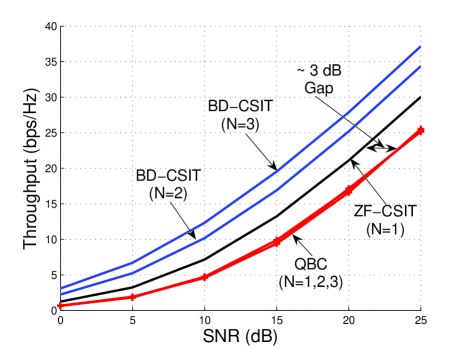
Figure 3: Sum rate of $M=K=6$ downlink channel

V-C Effect of Receiver Estimation Error

Although the analysis until now has assumed perfect CSI at the mobiles, a practical system always has some level of receiver error. We consider the scenario where a shared pilot sequence is used to train the mobiles. If $\beta M$ downlink pilots are used ($\beta\geq 1$ pilots per transmit antenna), channel estimation at the $k$-th mobile is performed on the basis of observation ${\bf G}_{k}=\sqrt{\beta P}{\bf H}_{k}+{\bf n}_{k}$. The MMSE estimate of ${\bf H}_{k}$ is $\hat{{\bf G}_{k}}=\frac{\sqrt{\beta P}}{1+\beta P}{\bf G}_{k}$, and the true channel matrix can be written as the sum of the MMSE estimate and independent estimation error:

$${\bf H}_{k}=\hat{{\bf G}_{k}}+{\bf e}_{k},$$ (21)

where ${\bf e}_{k}$ is white Gaussian noise, independent of the estimate $\hat{{\bf G}_{k}}$, with per-component variance $(1+\beta P)^{-1}$. After computing the channel estimate $\hat{{\bf G}_{k}}$, the mobile performs QBC on the basis of the estimate $\hat{{\bf G}_{k}}$ to determine the combining vector ${\boldsymbol{\gamma}}_{k}$. As a result, the quantization vector $\hat{{\bf h}_{k}}$ very accurately quantizes the vector $\hat{{\bf G}_{k}}{\boldsymbol{\gamma}}_{k}$, which is the mobile’s estimate of the effective channel output, while the actual effective channel is given by ${\bf h}^{\textrm{eff}}_{k}={\bf H}_{k}{\boldsymbol{\gamma}}_{k}$.

For simplicity we assume that coherent communication is possible, and therefore the long-term average throughput is again $E[\log_{2}(1+SINR_{k})]$ where the same expression for SINR given in (16) applies. The general throughput analysis in Section V still applies, and in particular, the rate gap upper bound given in Theorem 1 still holds if the expected quantization error takes into account the effect of receiver noise. As shown in Appendix C, the approximate rate loss with receiver error is:

$$\Delta R(P) \approx \log_{2}e\left(\sum_{l=M-N+1}^{M-1}\frac{1}{l}\right)+\log_{2}\left(1\!+\!P\cdot\left(\frac{M\!-\!N\!+\!1}{M}\right)2^{-\frac{B}{M-N}}{M\!-\!1\choose N\!-\!1}^{-\frac{1}{M-N}}+\frac{1}{\beta}\right).$$ (22)

Comparing this expression to (19) we see that estimation error leads only to the introduction of an additional $\frac{1}{\beta}$ term. If feedback is scaled according to (20) the rate loss is $\log_{2}(b+\beta^{-1})$ rather than $\log_{2}(b)$. In Figure 4 the throughput of a 4 mobile system with $M=4$ and $N=2$ is plotted for perfect CSIT/CSIR and for QBC performed on the basis of perfect CSIR ($\beta=\infty$) and imperfect CSIR for $\beta=1$ and $\beta=2$. Estimation error causes non-negligible degradation, but the loss decreases rather quickly with $\beta$ (which can be increased at a reasonable resource cost because pilots are shared).

Figure 4: Combining with Imperfect CSIR: $M=4$, $N=2$, $K=4$, $B$ scaled with SNR

VI Performance Comparisons

In this section we compare the throughput of QBC to other receive combining techniques and to limited feedback-based block diagonalization. For all results on receiving combining, the user selection algorithm of [7] is applied assuming limited feedback ($B$ bits) regarding the direction of the effective channel and perfect knowledge of the effective channel norm. We first describe these alternative approaches and then discuss some numerical results.

VI-A Alternate Combining Techniques

The optimal receive combining technique for a point-to-point MIMO channel in a limited feedback setting is to select the quantization vector that maximizes received power [3]:

$$\hat{{\bf h}}_{k} = \textrm{arg}\max_{{\bf w}={\bf w}_{1},\ldots,{\bf w}_{2^{B}}}||{\bf H}_{k}^{H}{\bf w}||^{2}.$$ (23)

Because this method roughly corresponds to maximum ratio combining, it is referred to as MRC. If BF vector ${\bf w}$ is used by the transmitter, received power is maximized by choosing $\boldsymbol{\gamma}=\frac{{\bf H}_{k}^{H}{\bf w}}{||{\bf H}_{k}^{H}{\bf w}||}$ [3], which yields ${\bf h}^{\textrm{eff}}_{k}={\bf H}_{k}\boldsymbol{\gamma}_{k}=\frac{{\bf H}_{k}{\bf H}_{k}^{H}{\bf w}_{k}}{||{\bf H}_{k}^{H}{\bf w}_{k}||}$. When $B$ is not very small, with high probability the quantization vector that maximizes $||{\bf H}_{k}^{H}{\bf w}||^{2}$ is the vector that is closest to the eigenvector corresponding to the maximum eigenvalue of ${\bf H}_{k}{\bf H}_{k}^{H}$. To see this, consider the maximization of $||{\bf H}_{k}^{H}{\bf w}||$ when ${\bf w}$ is constrained to have unit norm but need not be selected from a finite codebook. This corresponds to the classical definition of the matrix norm, and the optimizing ${\bf w}$ is in the direction of the maximum singular value of ${\bf H}_{k}$. When $B$ is not too small, the quantization error is very small and as a result the solution to (23) is extremely close to $||{\bf H}_{k}||^{2}$. As a result, selecting the quantization vector according to the criteria in (23) is roughly equivalent to directly finding the quantization vector that is closest to the direction of the maximum singular value of ${\bf H}_{k}$.

The maximum singular value of ${\bf H}_{k}$ can be directly quantized if the mobile first selects the combiner weights $\boldsymbol{\gamma}_{k}$ such that the effective channel ${\bf h}^{\textrm{eff}}_{k}={\bf H}_{k}\boldsymbol{\gamma}_{k}$ is in the direction of the maximum singular value, which corresponds to selecting $\boldsymbol{\gamma}_{k}$ equal to the eigenvector corresponding to the maximum eigenvalue of the $N\times N$ matrix ${\bf H}_{k}^{H}{\bf H}_{k}$, and then finds the quantization vector closest to ${\bf h}^{\textrm{eff}}_{k}$. The effective channel norm satisfies $||{\bf h}^{\textrm{eff}}_{k}||^{2}=||{\bf H}_{k}||^{2}$, which can be reasonably approximated as a scaled version of a $\chi^{2}_{2MN}$ random variable [15]. Therefore the norm of the effective channel is large, but notice that the quantization procedure reduces to standard vector quantization, for which the error is roughly $2^{-\frac{B}{M-1}}$.

In Figure 5, numerically computed values of the quantization error ($\log_{2}(E[\sin^{2}(\angle({\bf h}^{\textrm{eff}}_{k},\hat{{\bf h}_{k}}))]$) are shown for QBC, antenna selection, MRC (corresponding to equation 23), and direct quantization of the maximum eigenvector, along with approximation $2^{-\frac{B}{M-1}}$ as well as the approximation from (18), for a $M=4$, $N=2$ channel. Note that the error of QBC is very well approximated by (18), and the exponential rate of decrease of the other techniques are all well approximated by $2^{-\frac{B}{M-1}}$.

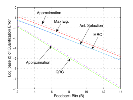
Figure 5: Quantization Error for Different Combining Techniques ($M=4$, $N=2$)

Each combining technique transforms the MIMO downlink into a vector downlink with a modified channel norm and quantization error. These techniques are summarized in Table I. The key point is that only QBC changes the exponent of the quantization error, which determines the rate at which feedback increases with SNR. When comparing these techniques note that the complexity of QBC and MRC are essentially the same: QBC and MRC require computation of $||{\bf Q}_{k}^{H}{\bf w}||^{2}$ and $||{\bf H}_{k}^{H}{\bf w}||^{2}$, respectively.

	Effective Channel Norm	Quantization Error
Single RX Antenna ($N=1$)	$\chi^{2}_{2M}$	$2^{-B/(M-1)}$
Antenna Selection	$\chi^{2}_{2M}$	$2^{-(B+\log_{2}N)/(M-1)}$
MRC	$\approx$ max eigenvalue	$2^{-B/(M-1)}$
Max Eigenvector	max eigenvalue	$2^{-B/(M-1)}$
QBC	$\chi^{2}_{2(M-N+1)}$	$2^{-B/(M-N)}$

TABLE I: Summary of Combining Techniques

VI-B Block Diagonalization

An alternative manner in which multiple receive antennas can be used is to extend the linear precoding structure of ZFBF to allow for transmission of multiple data streams to each mobile. Block diagonalization (BD) selects precoding matrices such multi-user interference is eliminated at each receiver, similar to ZFBF. In order to select appropriate precoding matrices, the transmitter must know the $N$-dimensional subspace spanned by each mobile channel ${\bf H}_{k}$. Thus an appropriate feedback strategy is to have each mobile quantize and feedback its channel subspace. The effect of limited feedback in this setting (assuming there are $\frac{M}{N}$ mobiles and equal power loading across users and streams is performed) was studied in [17]. In order to achieve a bounded rate loss relative to a perfect CSIT (BD) system, feedback (per mobile) needs to scale approximately as $N(M-N)\log_{2}P$. Thus, the aggregate feedback load summed over $\frac{M}{N}$ mobiles is approximately $M(M-N)\log_{2}P$, which is (approximately) the same as the aggregate feedback in a QBC system in which each of the $M$ mobiles uses $B\approx(M-N)\log_{2}P$. Thus, there is a rough equivalence between QBC and BD in terms of feedback scaling, and this is later confirmed by our numerical results.

It is also possible to perform user and stream selection when BD is used, and [18] presents an extension of the algorithm of [7] to the multiple receive antenna setting (referred to as maximum eigenmode transmission, or MET). In essence, MET treats each mobile’s $N$ eigenmodes as a different single antenna receiver and selects eigenmodes in a greedy fashion using the approach of [7]. Thus, in a limited feedback setting a reasonable strategy is to have each user separately quantize the directions of its $N$ eigenvectors and also feed back the corresponding eigenvalues.

VI-C Numerical Results

In Figures 6 and 7 throughput curves are shown for a 4 transmit antenna, 2 receive antenna ($M=4$, $N=2$) system with $K=4$ mobiles. Sum rate is plotted for three different combining techniques (QBC, antenna selection, and MRC) and for a vector downlink channel ($N=1$); the BD curves are discussed in later paragraphs. In Fig. 6, $B$ (per mobile) is scaled according to (20), i.e., roughly as $(M-N)\log_{2}P$, while in Fig. 7 each mobile uses 10 bits of feedback. As expected, the throughput of antenna selection, MRC, and the single antenna system all lag behind QBC in Fig. 6, particularly at high SNR. This is because the $(M-N)\log_{2}P$ scaling of feedback is simply not sufficient to maintain good performance if these techniques are used. To be more precise, the quantization error goes to zero slower than $\frac{1}{P}$ which corresponds to interference power that increases with SNR, and thus a reduction in the slope (i.e., multiplexing gain) of these curves. In Fig. 7, MRC outperforms QBC for SNR less than approximately 12 dB because signal power is more important than quantization error (i.e., interference power), i.e., the system is not yet interference-limited. However, at higher SNR’s QBC outperforms MRC because of the increased importance of quantization error.

Figure 6: Different Combining Techniques: $M=4$, $N=2$, $K=4$, $B$ scaled with SNR

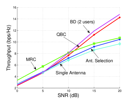
Figure 7: Different Combining Techniques: $M=4$, $N=2$, $K=4$, $B=10$

Figures 6 and 7 also include plots of the throughput of a BD system. In this system, 2 of the 4 users are randomly selected to feedback subspace information, and equal power BD with no selection is used to send 2 streams to each of these mobiles, for a total of 4 streams. In order to equalize the aggregate feedback load, each of the 2 users is allocated double the feedback budget of the combining-based systems; this corresponds to using two times the scaling of (20) in Fig. 6 and 20 bits per mobile in Fig. 7. BD performs slightly better than QBC in both figures, but we later see that this advantage is lost for larger $K$.

Figures 8 displays throughput for a 4 transmit antenna, 2 receive antenna ($M=4$, $N=2$) system at 10 dB against $K$, the number of mobiles. Capacity refers to the sum capacity of the system (with CSIT), MET-CSIT is the throughput achieved using the MET algorithm on the basis of CSIT[18], and ZF-CSIT is the throughput of a vector downlink with CSIT and user selection [7]. Below these are four limited feedback curves for 10 bits of feedback per mobile. The first three, QBC, MRC, and antenna selection, correspond to different combining techniques, while MET-FB corresponds to performing MET on the basis of 5 bit quantization of each eigenmode (10 bits total feedback per mobile). QBC achieves significantly higher throughput than MRC or antenna selection, particularly for larger values of $K$. The ZF-CSIT curve is shown because it serves as an upper bound on the performance of QBC, and the gap between the two is quite reasonable even for $B=10$. MET-FB is seen to perform extremely poorly: this is not too surprising because the MET algorithm is likely to only choose the strongest eigenmode of a few users [18], and thus half of the feedback is essentially wasted on quantization of each user’s weakest eigenmode. This motivates dedicating all 10 bits to quantization of the strongest eigenmode, but note that this essentially corresponds to MRC, which is outperformed by QBC. The huge gap between MET-CSIT and MET-FB indicates that MET has the potential to provide excellent performance, but extremely high levels of feedback may be necessary to realize MET’s potential.

Finally, Figure 9 shows throughput versus number of users $K$ for a 6 transmit antenna ($M=6$) channel with either 1 or 2 receive antennas. Sum capacity for $N=1$ and $N=2$ is plotted, along with the sum rate of a perfect-CSIT TDMA system in which only the receiver with the largest point-to-point capacity is selected for transmission. The ZF and QBC curves correspond to systems with user selection and either single receive antennas or quantization-based combining, respectively, for feedback levels of 10, 15, and 20 bits per mobile. For each feedback level, an additional receive antenna with QBC provides a significant throughput gain relative to a single receive antenna system. Furthermore, QBC significantly outperforms TDMA ($N=2$) for $B=15$ or $B=20$, and provides an advantage over TDMA for $B=10$ when the number of users is sufficiently large. Note, however, that there is a significant gap between QBC and $N=2$ capacity even when 20 bits of feedback are used; this indicates that there may be room for significant improvement beyond QBC.

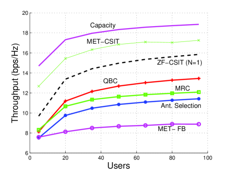
Figure 8: Combining and User Selection: $M=4$, $N=2$, $B=10$

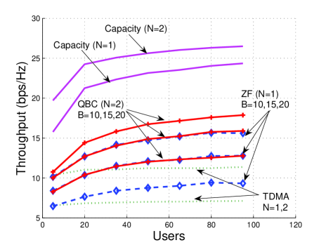
Figure 9: Combining and User Selection: $M=6$, $N=1,2$

VII Conclusion

The performance of multi-user MIMO techniques such as zero-forcing beamforming critically depend on the accuracy of the channel state information provided to the transmitter. In this paper, we have shown that receive antenna combining can be used to reduce channel quantization error in limited feedback MIMO downlink channels, and thus significantly reduce channel feedback requirements. Unlike traditional maximum-ratio combining techniques that maximize received signal power, the proposed quantization-based combining technique minimizes quantization error, which translates into minimization of multi-user interference power.

Antenna combining is just one method by which multiple receive antennas can be used in the MIMO downlink. It is also possible to transmit multiple streams to each mobile, or to use receive antennas for interference cancellation if the structure of the transmitted signal is known to the mobile. It remains to be seen which of these techniques is most beneficial in practical wireless systems when channel feedback resources and complexity requirements are carefully accounted for.

Appendix A Proof of Theorem 1

Plugging the rate expressions into the definition of $\Delta(P)$, we have $\Delta(P)=\Delta_{a}+\Delta_{b}$ where

$$\Delta_{a} = E_{{\bf H}}\left[\log_{2}\left(1+\rho|{\bf h}_{k}^{H}{\bf v}_{ZF,k}|^{2}\right)\right]-E_{{\bf H},\bf{W}}\left[\log_{2}\left(1+\sum_{j=1}^{M}\rho|({\bf h}^{\textrm{eff}}_{k})^{H}{\bf v}_{j}|^{2}\right)\right]$$

$$\Delta_{b} = E_{{\bf H},\bf{W}}\left[\log_{2}\left(1+\sum_{j\neq k}\rho|({\bf h}^{\textrm{eff}}_{k})^{H}{\bf v}_{j}|^{2}\right)\right],$$

where $\rho\triangleq\frac{P}{M}$. To upper bound $\Delta_{a}$, we define normalized vectors $\tilde{{\bf h}_{k}}={\bf h}_{k}/||{\bf h}_{k}||$ and $\tilde{{\bf h}^{\textrm{eff}}_{k}}={\bf h}^{\textrm{eff}}_{k}/||{\bf h}^{\textrm{eff}}_{k}||$, and note that the norm and directions of ${\bf h}_{k}$ and of ${\bf h}^{\textrm{eff}}_{k}$ are independent. Using this we have:

$$E_{{\bf H},\bf{W}}\left[\log_{2}\left(1+\sum_{j=1}^{M}\rho|({\bf h}^{\textrm{eff}}_{k})^{H}{\bf v}_{j}|^{2}\right)\right] \geq E_{{\bf H},\bf{W}}\left[\log_{2}\left(1+\rho|({\bf h}^{\textrm{eff}}_{k})^{H}{\bf v}_{k}|^{2}\right)\right]$$ (24)

$$= E_{{\bf H},\bf{W}}\left[\log_{2}\left(1+\rho||{\bf h}^{\textrm{eff}}_{k}||^{2}|\tilde{{\bf h}^{\textrm{eff}}_{k}}^{H}{\bf v}_{k}|^{2}\right)\right]$$

$$= E_{{\bf H}}\left[\log_{2}\left(1+\rho X_{\beta}||{\bf h}_{k}||^{2}|\tilde{{\bf h}_{k}}^{H}{\bf v}_{ZF,k}|^{2}\right)\right],$$

where $X_{\beta}$ is $\beta(M-N+1,N-1)$. Since the BF vector ${\bf v}_{ZF,k}$ is chosen orthogonal to the $(M-1)$ other channel vectors $\{{\bf h}_{j}\}_{j\neq k}$, each of which is an iid isotropic vector, it is isotropic and is independent of $\tilde{{\bf h}_{k}}$. By Lemma 2 the same is also true of ${\bf v}_{k}$ and $\tilde{{\bf h}^{\textrm{eff}}_{k}}$, and therefore we can substitute $|\tilde{{\bf h}_{k}}^{H}{\bf v}_{ZF,k}|^{2}$ for $|({\bf h}^{\textrm{eff}}_{k})^{H}{\bf v}_{k}|^{2}$. Finally, note that the product $X_{\beta}||{\bf h}_{k}||^{2}$ is $\chi^{2}_{2(M-N+1)}$ because $||{\bf h}_{k}||^{2}$ is $\chi^{2}_{2M}$, and therefore $X_{\beta}||{\bf h}_{k}||^{2}$ and $||{\bf h}^{\textrm{eff}}_{k}||^{2}$ have the same distribution. Using (24) we get:

$$\Delta_{a}\leq E_{{\bf H}}\left[\log_{2}\left(\frac{1+\rho||{\bf h}_{k}||^{2}|\tilde{{\bf h}_{k}}^{H}{\bf v}_{ZF,k}|^{2}}{1+\rho X_{\beta}||{\bf h}_{k}||^{2}|\tilde{{\bf h}_{k}}^{H}{\bf v}_{ZF,k}|^{2}}\right)\right]\leq-E\left[\log_{2}\left(X_{\beta}\right)\right]=\log_{2}e\left(\sum_{l=M-N+1}^{M-1}\frac{1}{l}\right),$$

where we have used $\log_{2}\left(X_{\beta}\right)=\log_{2}\left(\frac{\chi^{2}_{2M}}{\chi^{2}_{2(M-N+1)}}\right)$ and results from [8] to to compute $E\left[\log_{2}\left(X_{\beta}\right)\right]$.

Finally, we upper bound $\Delta_{b}$ using Jensen’s inequality:

$$\Delta_{b} \leq \log_{2}\left(1+E\left[\sum_{j\neq k}\rho|({\bf h}^{\textrm{eff}}_{k})^{H}{\bf v}_{j}|^{2}\right]\right)$$

$$= \log_{2}\left(1+\rho(M-1)E\left[||({\bf h}^{\textrm{eff}}_{k})||^{2}\right]E\left[|(\tilde{{\bf h}^{\textrm{eff}}}_{k})^{H}{\bf v}_{j}|^{2}\right]\right)$$

$$= \log_{2}\left(1+\rho(M-1)(M-N+1)E\left[|(\tilde{{\bf h}^{\textrm{eff}}}_{k})^{H}{\bf v}_{j}|^{2}\right]\right)$$

$$= \log_{2}\left(1+\rho(M-N+1)E\left[\sin^{2}\left(\angle\left(\tilde{{\bf h}^{\textrm{eff}}}_{k},{\bf h}_{k}\right)\right)\right]\right),$$

where the final step uses Lemma 2 of [2] to get $E\left[|(\tilde{{\bf h}^{\textrm{eff}}}_{k})^{H}{\bf v}_{j}|^{2}\right]=\frac{1}{M-1}E\left[\sin^{2}\left(\angle\left(\tilde{{\bf h}^{\textrm{eff}}}_{k},{\bf h}_{k}\right)\right)\right]$.

Appendix B Generation of Numerical Results

Rather than performing brute force simulation of RVQ, which becomes infeasible for $B$ larger than 15 or 20, the statistics of RVQ can be exploited to efficiently and exactly emulate the quantization process:

1. Draw a realization of the quantization error $Z$ according to its known CDF (Lemma 1).

2. Draw a realization of the corresponding quantization vector according to:

   $$\hat{{\bf h}_{k}}=\left(\sqrt{1-Z}\right){\bf u}+\sqrt{Z}{\bf s}$$

   where ${\bf u}$ is isotropic in span(${\bf H}_{k}$), ${\bf s}$ is isotropic in the nullspace of span(${\bf H}_{k}$), with ${\bf u}$, ${\bf s}$ independent.

These steps exactly emulate step 2 of QBC. The same procedure can also be used to emulate antenna selection, quantization of the maximum eigenvector, and no combining ($N=1$). Because the CDF of the quantization error is not known for MRC, MRC results are generated using brute force RVQ.

Appendix C Rate Gap with Receiver Estimation Error

We bound the rate gap using the technique of [13]. We first restate the result of Theorem 1 in terms of the interference terms $E\left[|({\bf h}^{\textrm{eff}}_{k})^{H}{\bf v}_{j}|^{2}\right]$:

$$\Delta R \leq \log_{2}e\left(\sum_{l=M-N+1}^{M-1}\frac{1}{l}\right)+\log_{2}\left(1+P\frac{M-1}{M}E\left[|({\bf h}^{\textrm{eff}}_{k})^{H}{\bf v}_{j}|^{2}\right]\right).$$ (25)

Using the representation of the channel matrix given in (21), we can write the interference term as:

$$({\bf h}^{\textrm{eff}}_{k})^{H}{\bf v}_{j} = \left({\bf H}_{k}{\boldsymbol{\gamma}}_{k}\right)^{H}{\bf v}_{j}=\left(\hat{{\bf G}_{k}}{\boldsymbol{\gamma}}_{k}\right)^{H}{\bf v}_{j}+\left({\bf e}_{k}{\boldsymbol{\gamma}}_{k}\right)^{H}{\bf v}_{j}.$$

The first term in the sum is statistically identical to the interference term when there is perfect CSIR, while the second term represents the additional interference due to the receiver estimation error. Because the noise and the channel estimate are each zero-mean and are independent we have:

$$E\left[|({\bf h}^{\textrm{eff}}_{k})^{H}{\bf v}_{j}|^{2}\right] = E\left[\left|\left(\hat{{\bf G}_{k}}{\boldsymbol{\gamma}}_{k}\right)^{H}{\bf v}_{j}\right|^{2}\right]+E\left[\left|\left({\bf e}_{k}{\boldsymbol{\gamma}}_{k}\right)^{H}{\bf v}_{j}\right|^{2}\right]$$

The first term comes from the perfect CSIR analysis and is equal to the product of $\frac{1}{M-1}$ and the expected quantization error with perfect CSIR. Because $\boldsymbol{\gamma}_{k}$ and ${\bf v}_{j}$ are each unit norm and ${\bf e}_{k}$ is independent of these two vectors, the quantity $\left({\bf e}_{k}{\boldsymbol{\gamma}}_{k}\right)^{H}{\bf v}_{j}$ is (zero-mean) complex Gaussian with variance $(1+\beta P)^{-1}$, which is less than $(1+\beta P)^{-1}$. We finally reach (22) by using the approximation for quantization error from (18) and plugging into (25), and noting that $(1+\beta P)^{-1}\approx(\beta P)^{-1}$.

References

- [1] D. Love, R. Heath, W. Santipach, and M. Honig, “What is the value of limited feedback for MIMO channels?” IEEE Communications Magazine, vol. 42, no. 10, pp. 54–59, Oct. 2004.
- [2] N. Jindal, “MIMO broadcast channels with finite rate feedback,” IEEE Trans. on Inform. Theory, vol. 52, no. 11, pp. 5045–5059, 2006.
- [3] D. Love, R. Heath, and T. Strohmer, “Grassmannian beamforming for multiple-input multiple-output wireless systems,” IEEE Trans. Inform. Theory, vol. 49, no. 10, pp. 2735–2747, Oct. 2003.
- [4] K. Mukkavilli, A. Sabharwal, E. Erkip, and B. Aazhang, “On beamforming with finite rate feedback in multiple-antenna systems,” IEEE Trans. Inform. Theory, vol. 49, no. 10, pp. 2562–2579, Oct. 2003.
- [5] W. Santipach and M. Honig, “Asymptotic capacity of beamforming with limited feedback,” in Proceedings of Int. Symp. Inform. Theory, July 2004, p. 290.
- [6] T. Yoo and A. Goldsmith, “On the optimality of multiantenna broadcast scheduling using zero-forcing beamforming,” IEEE Journal on Selected Areas in Communications, vol. 24, no. 3, pp. 528–541, 2006.
- [7] G. Dimic and N. Sidiropoulos, “On downlink beamforming with greedy user selection: Performance analysis and simple new algorithm,” IEEE Trans. Sig. Proc., vol. 53, no. 10, pp. 3857–3868, October 2005.
- [8] A. Tulino and S. Verdu, “Random matrix theory and wireless communications,” Foundations and Trends in Communications and Information Theory, vol. 1, no. 1, 2004.
- [9] A. K. Gupta and S. Nadarajah, Handbook of Beta Distribution and Its Applications. CRC, 2004.
- [10] J. Winters, J. Salz, and R. Gitlin, “The impact of antenna diversity on the capacity of wireless communication systems,” IEEE Trans. on Communications, vol. 42, no. 234, pp. 1740–1751, 1994.
- [11] Q. Spencer, A. Swindlehurst, and M. Haardt, “Zero-forcing methods for downlink spatial multiplexing in multiuser MIMO channels,” IEEE Trans. Sig. Proc., vol. 52, no. 2, pp. 461–471, 2004.
- [12] J. Lee and N. Jindal, “High SNR analysis for MIMO broadcast channels: Dirty paper coding vs. linear precoding,” to appear in IEEE Trans. Inform. Theory, 2007.
- [13] G. Caire, N. Jindal, M. Kobayashi, and N. Ravindran, “Quantized vs. analog feedback for the MIMO downlink: A comparison between zero-forcing based achievable rates,” in Proceedings of Int. Symp. Inform. Theory, June 2007.
- [14] T. Yoo, N. Jindal, and A. Goldsmith, “Finite-rate feedback MIMO broadcast channels with a large number of users,” 2007, to appear in IEEE J. Sel. Areas on Commun.
- [15] A. Paulraj, D. Gore, and R. Nabar, Introduction to Space-Time Wireless Communications. Cambridge University Press, 2003.
- [16] M. Trivellato, H. Huang, and F. Boccardi, “Antenna combining and codebook design for MIMO broadcast channel with limited feedback,” in Proc. Asilomar Conf. on Sig. and Systems, Nov. 2007.
- [17] N. Ravindran and N. Jindal, “MIMO broadcast channels with block diagonalization and finite rate feedback,” in Proc. ICASSP, April 2007.
- [18] F. Boccardi and H. Huang, “A near-optimum technique using linear precoding for the MIMO broadcast channel,” in Proc. ICASSP, April 2007.