The Measurement Calculus

Abstract

Measurement-based quantum computation has emerged from the physics community as a new approach to quantum computation where the notion of measurement is the main driving force of computation. This is in contrast with the more traditional circuit model which is based on unitary operations. Among measurement-based quantum computation methods, the recently introduced one-way quantum computer [RB01] stands out as fundamental.

We develop a rigorous mathematical model underlying the one-way quantum computer and present a concrete syntax and operational semantics for programs, which we call patterns, and an algebra of these patterns derived from a denotational semantics. More importantly, we present a calculus for reasoning locally and compositionally about these patterns. We present a rewrite theory and prove a general standardization theorem which allows all patterns to be put in a semantically equivalent standard form. Standardization has far-reaching consequences: a new physical architecture based on performing all the entanglement in the beginning, parallelization by exposing the dependency structure of measurements and expressiveness theorems.

Furthermore we formalize several other measurement-based models e.g. Teleportation, Phase and Pauli models and present compositional embeddings of them into and from the one-way model. This allows us to transfer all the theory we develop for the one-way model to these models. This shows that the framework we have developed has a general impact on measurement-based computation and is not just particular to the one-way quantum computer.

1 Introduction

The emergence of quantum computation has changed our perspective on many fundamental aspects of computing: the nature of information and how it flows, new algorithmic design strategies and complexity classes and the very structure of computational models [NC00]. New challenges have been raised in the physical implementation of quantum computers. This paper is a contribution to a nascent discipline: quantum programming languages.

This is more than a search for convenient notation, it is an investigation into the structure, scope and limits of quantum computation. The main issues are questions about how quantum processes are defined, how quantum algorithms compose, how quantum resources are used and how classical and quantum information interact.

Quantum computation emerged in the early 1980s with Feynman’s observations about the difficulty of simulating quantum systems on a classical computer. This hinted at the possibility of turning around the issue and exploiting the power of quantum systems to perform computational tasks more efficiently than was classically possible. In the mid 1980s Deutsch [Deu87] and later Deutsch and Jozsa [DJ92] showed how to use superposition – the ability to produce linear combinations of quantum states – to obtain computational speedup. This led to interest in algorithm design and the complexity aspects of quantum computation by computer scientists. The most dramatic results were Shor’s celebrated polytime factorization algorithm [Sho94] and Grover’s sublinear search algorithm [Gro98]. Remarkably one of the problematic aspects of quantum theory, the presence of non-local correlation – an example of which is called “entanglement” – turned out to be crucial for these algorithmic developments.

If efficient factorization is indeed possible in practice, then much of cryptography becomes insecure as it is based on the difficulty of factorization. However, entanglement makes it possible to design unconditionally secure key distribution [BB84, Eke91]. Furthermore, entanglement led to the remarkable – but simple – protocol for transferring quantum states using only classical communication [BBC⁺93]; this is the famous so-called “teleportation” protocol. There continues to be tremendous activity in quantum cryptography, algorithmic design, complexity and information theory. Parallel to all this work there has been intense interest from the physics community to explore possible implementations, see, for example, [NC00] for a textbook account of some of these ideas.

On the other hand, only recently has there been significant interest in quantum programming languages; i.e. the development of formal syntax and semantics and the use of standard machinery for reasoning about quantum information processing. The first quantum programming languages were variations on imperative probabilistic languages and emphasized logic and program development based on weakest preconditions [SZ00, Ö01]. The first definitive treatment of a quantum programming language was the flowchart language of Selinger [Sel04b]. It was based on combining classical control, as traditionally seen in flowcharts, with quantum data. It also gave a denotational semantics based on completely positive linear maps. The notion of quantum weakest preconditions was developed in [DP06]. Later people proposed languages based on quantum control [AG05]. The search for a sensible notion of higher-type computation [SV05, vT04] continues, but is problematic [Sel04c].

A related recent development is the work of Abramsky and Coecke [AC04, Coe04] where they develop a categorical axiomatization of quantum mechanics. This can be used to verify the correctness of quantum communication protocols. It is very interesting from a foundational point of view and allows one to explore exactly what mathematical ingredients are required to carry out certain quantum protocols. This has also led to work on a categorical quantum logic [AD04].

The study of quantum communication protocols has led to formalizations based on process algebras [GN05, JL04] and to proposals to use model checking for verifying quantum protocols. A survey and a complete list of references on this subject up to 2005 is available [Gay05].

These ideas have proven to be of great utility in the world of classical computation. The use of logics, type systems, operational semantics, denotational semantics and semantic-based inference mechanisms have led to notable advances such as: the use of model checking for verification, reasoning compositionally about security protocols, refinement-based programming methodology and flow analysis.

The present paper applies this paradigm to a very recent development: measurement-based quantum computation. None of the cited research on quantum programming languages is aimed at measurement-based computation. On the other hand, the work in the physics literature does not clearly separate the conceptual layers of the subject from implementation issues. A formal treatment is necessary to analyze the foundations of measurement-based computation.

So far the main framework to explore quantum computation has been the circuit model [Deu89], based on unitary evolution. This is very useful for algorithmic development and complexity analysis [BV97]. There are other models such as quantum Turing machines [Deu85] and quantum cellular automata [Wat95, vD96, DS96, SW04]. Although they are all proved to be equivalent from the point of view of expressive power, there is no agreement on what is the canonical model for exposing the key aspects of quantum computation.

Recently physicists have introduced novel ideas based on the use of measurement and entanglement to perform computation [GC99, RB01, RBB03, Nie03]. This is very different from the circuit model where measurement is done only at the end to extract classical output. In measurement-based computation the main operation to manipulate information and control computation is measurement. This is surprising because measurement creates indeterminacy, yet it is used to express deterministic computation defined by a unitary evolution.

The idea of computing based on measurements emerged from the teleportation protocol [BBC⁺93]. The goal of this protocol is for an agent to transmit an unknown qubit to a remote agent without actually sending the qubit. This protocol works by having the two parties share a maximally entangled state called a Bell pair. The parties perform local operations – measurements and unitaries – and communicate only classical bits. Remarkably, from this classical information the second party can reconstruct the unknown quantum state. In fact one can actually use this to compute via teleportation by choosing an appropriate measurement [GC99]. This is the key idea of measurement-based computation.

It turns out that the above method of computing is actually universal. This was first shown by Gottesman and Chuang [GC99] who used two-qubit measurements and given Bell pairs. Later Nielsen [Nie03] showed that one could do this with only 4-qubit measurements with no prior Bell pairs, however this works only probabilistically. Leung [Leu04] improved this to two qubits, but her method also works only probabilistically. Later Perdrix and Jorrand [Per03, PJ04] gave the minimal set measurements to perform universal quantum computing – but still in the probabilistic setting – and introduced the state-transfer and measurement-based quantum Turing machine. Finally the one-way computer was invented by Raussendorf and Briegel [RB01, RB02] which used only single-qubit measurements with a particular multi-party entangled state, the cluster state.

More precisely, a computation consists of a phase in which a collection of qubits are set up in a standard entangled state. Then measurements are applied to individual qubits and the outcomes of the measurements may be used to determine further measurements. Finally – again depending on measurement outcomes – local unitary operators, called corrections, are applied to some qubits; this allows the elimination of the indeterminacy introduced by measurements. The phrase “one-way” is used to emphasize that the computation is driven by irreversible measurements.

There are at least two reasons to take measurement-based models seriously: one conceptual and one pragmatic. The main pragmatic reason is that the one-way model is believed by physicists to lend itself to easier implementations [Nie04, CAJ05, BR05, TPKV04, TPKV06, WkJRR⁺05, KPA06, BES05, CCWD06, BBFM06]. Physicists have investigated various properties of the cluster state and have accrued evidence that the physical implementation is scalable and robust against decoherence [Sch03, HEB04, DAB03, dNDM04b, dNDM04a, MP04, GHW05, HDB05, DHN06]. Conceptually the measurement-based model highlights the role of entanglement and separates the quantum and classical aspects of computation; thus it clarifies, in particular, the interplay between classical control and the quantum evolution process.

Our approach to understanding the structural features of measurement-based computation is to develop a formal calculus. One can think of this as an “assembly language” for measurement-based computation. Ours is the first programming framework specifically based on the one-way model. We first develop a notation for such classically correlated sequences of entanglements, measurements, and local corrections. Computations are organized in patterns, and we give a careful treatment of the composition and tensor product (parallel composition) of patterns. We show next that such pattern combinations reflect the corresponding combinations of unitary operators. An easy proof of universality follows.

So far, this is primarily a clarification of what was already known from the series of papers introducing and investigating the properties of the one-way model [RB01, RB02, RBB03]. However, we work here with an extended notion of pattern, where inputs and outputs may overlap in any way one wants them to, and this results in more efficient – in the sense of using fewer qubits – implementations of unitaries. Specifically, our universal set consists of patterns using only 2 qubits. From it we obtain a 3 qubit realization of the $R_{z}$ rotations and a 14 qubit realization for the controlled-$U$ family: a significant reduction over the hitherto known implementations.

The main point of this paper is to introduce a calculus of local equations over patterns that exploits some special algebraic properties of the entanglement, measurement and correction operators. More precisely, we use the fact that that 1-qubit $XY$ measurements are closed under conjugation by Pauli operators and the entanglement command belongs to the normalizer of the Pauli group; these terms are explained in the appendix. We show that this calculus is sound in that it preserves the interpretation of patterns. Most importantly, we derive from it a simple algorithm by which any general pattern can be put into a standard form where entanglement is done first, then measurements, then corrections. We call this standardization.

The consequences of the existence of such a procedure are far-reaching. Since entangling comes first, one can prepare the entire entangled state needed during the computation right at the start: one never has to do “on the fly” entanglements. Furthermore, the rewriting of a pattern to standard form reveals parallelism in the pattern computation. In a general pattern, one is forced to compute sequentially and to strictly obey the command sequence, whereas, after standardization, the dependency structure is relaxed, resulting in lower computational depth complexity. Last, the existence of a standard form for any pattern also has interesting corollaries beyond implementation and complexity matters, as it follows from it that patterns using no dependencies, or using only the restricted class of Pauli measurements, can only realize a unitary belonging to the Clifford group, and hence can be efficiently simulated by a classical computer [Got97].

As we have noted before, there are other methods for measurement-based quantum computing: the teleportation technique based on two-qubit measurements and the state-transfer approach based on single qubit measurements and incomplete two-qubit measurements. We will analyze the teleportation model and its relation to the one-way model. We will show how our calculus can be smoothly extended to cover this case as well as new models that we introduce in this paper. We get several benefits from our treatment. We get a workable syntax for handling the dependencies of operators on previous measurement outcomes just by mimicking the one obtained in the one-way model. This has never been done before for the teleportation model. Furthermore, we can use this embedding to obtain a standardization procedure for the models. Finally these extended calculi can be compositionally embedded back in the original one-way model. This clarifies the relation between different measurement-based models and shows that the one-way model of Raussendorf and Briegel is the canonical one.

This paper develops the one-way model ab initio but certain concepts that the reader may be unfamiliar with: qubits, unitaries, measurements, Pauli operators and the Clifford group are in an appendix. These are also readily accessible through the very thorough book of Nielsen and Chuang [NC00].

In the next section we define the basic model, followed by its operational and denotational semantics, for completeness a simple proof of universality is given in section 4, this has appeared earlier in the physics literature [DKP05], in section 5 we develop the rewrite theory and prove the fundamental standardization theorem. In section 6 we develop several examples that illustrate the use of our calculus in designing efficient patterns. In section 7 we prove some theorems about the expressive power of the calculus in the absence of adaptive measurements. In section 8 we discuss other measurement-based models and their compositional embedding to and from the one-way model. In section 9 we discuss further directions and some more related work. In the appendix we review basic notions of quantum mechanics and quantum computation.

2 Measurement Patterns

We first develop a notation for 1-qubit measurement based computations. The basic commands one can use in a pattern are:

• 1-qubit auxiliary preparation $N_{i}$

• 2-qubit entanglement operators $E_{ij}$

• 1-qubit measurements ${M}_{i}^{\alpha}$

• and 1-qubit Pauli operators corrections $X_{i}$ and $Z_{i}$

The indices $i$, $j$ represent the qubits on which each of these operations apply, and $\alpha$ is a parameter in $[0,2\pi]$. Expressions involving angles are always evaluated modulo $2\pi$. These types of command will be referred to as $N$, $E$, $M$ and $C$. Sequences of such commands, together with two distinguished – possibly overlapping – sets of qubits corresponding to inputs and outputs, will be called measurement patterns, or simply patterns. These patterns can be combined by composition and tensor product.

Importantly, corrections and measurements are allowed to depend on previous measurement outcomes. We shall prove later that patterns without these classical dependencies can only realize unitaries that are in the Clifford group. Thus, dependencies are crucial if one wants to define a universal computing model; that is to say, a model where all unitaries over $\otimes^{n}{\mathbb{C}}^{2}$ can be realized. It is also crucial to develop a notation that will handle these dependencies. This is what we do now.

2.1 Commands

Preparation $N_{i}$ prepares qubit $i$ in state ${|}+\rangle_{i}$. The entanglement commands are defined as $E_{ij}:=\mathop{\wedge}\hskip-1.72218ptZ_{ij}$ (controlled-$Z$), while the correction commands are the Pauli operators $X_{i}$ and $Z_{i}$.

Measurement ${M}_{i}^{\alpha}$ is defined by orthogonal projections on

$$\begin{array}[c]{lllllllllllllll}{|}\hskip-0.43057pt+_{\alpha}\rangle&:=&\frac{1}{\sqrt{2}}({|}0\rangle+e^{i\alpha}{|}1\rangle)\\ {|}\hskip-0.43057pt-_{\alpha}\rangle&:=&\frac{1}{\sqrt{2}}({|}0\rangle-e^{i\alpha}{|}1\rangle)\end{array}$$

followed by a trace-out operator. The parameter $\alpha\in[0,2\pi]$ is called the angle of the measurement. For $\alpha=0$, $\alpha=\frac{\pi}{2}$, one obtains the $X$ and $Y$ Pauli measurements. Operationally, measurements will be understood as destructive measurements, consuming their qubit. The outcome of a measurement done at qubit $i$ will be denoted by $s_{i}\in{\mathbb{Z}}_{2}$. Since one only deals here with patterns where qubits are measured at most once (see condition (D1) below), this is unambiguous. We take the specific convention that $s_{i}=0$ if under the corresponding measurement the state collapses to ${|}\hskip-0.43057pt+_{\alpha}\rangle$, and $s_{i}=1$ if to ${|}\hskip-0.43057pt-_{\alpha}\rangle$.

Outcomes can be summed together resulting in expressions of the form $s=\sum_{i\in I}s_{i}$ which we call signals, and where the summation is understood as being done in ${\mathbb{Z}}_{2}$. We define the domain of a signal as the set of qubits on which it depends.

As we have said before, both corrections and measurements may depend on signals. Dependent corrections will be written $X_{i}^{s}$ and $Z_{i}^{s}$ and dependent measurements will be written ${}^{t}[{M}_{i}^{\alpha}]^{s}$, where $s,t\in{\mathbb{Z}}_{2}$ and $\alpha\in[0,2\pi]$. The meaning of dependencies for corrections is straightforward: $X_{i}^{0}=Z_{i}^{0}=I$, no correction is applied, while $X_{i}^{1}=X_{i}$ and $Z_{i}^{1}=Z_{i}$. In the case of dependent measurements, the measurement angle will depend on $s$, $t$ and $\alpha$ as follows:

$${}^{t}[{M}_{i}^{\alpha}]^{s} := {M}_{i}^{(-1)^{s}\alpha+t\pi}$$ (1)

so that, depending on the parities of $s$ and $t$, one may have to modify the $\alpha$ to one of $-\alpha$, $\alpha+\pi$ and $-\alpha+\pi$. These modifications correspond to conjugations of measurements under $X$ and $Z$:

$$X_{i}{M}_{i}^{{\alpha}}X_{i} = {M}_{i}^{{-\alpha}}$$ (2)

$$Z_{i}{M}_{i}^{{\alpha}}Z_{i} = {M}_{i}^{{\alpha+\pi}}$$ (3)

accordingly, we will refer to them as the $X$ and $Z$-actions. Note that these two actions commute, since $-\alpha+\pi=-\alpha-\pi$ up to $2\pi$, and hence the order in which one applies them does not matter.

As we will see later, relations (2) and (3) are key to the propagation of dependent corrections, and to obtaining patterns in the standard entanglement, measurement and correction form. Since the measurements considered here are destructive, the above equations actually simplify to

$${M}_{i}^{{\alpha}}X_{i} = {M}_{i}^{{-\alpha}}$$ (4)

$${M}_{i}^{{\alpha}}Z_{i} = {M}_{i}^{{\alpha-\pi}}$$ (5)

Another point worth noticing is that the domain of the signals of a dependent command, be it a measurement or a correction, represents the set of measurements which one has to do before one can determine the actual value of the command.

We have completed our catalog of basic commands, including dependent ones, and we turn now to the definition of measurement patterns. For convenient reference, the language syntax is summarized in Figure  1.

$$\begin{array}[]{lllr}S&:=&0,\,1,\,s_{i},\,S+S&\quad\hbox{Signals}\\ A&:=&N_{i}&\quad\hbox{Preparations}\\ &&E_{ij}&\quad\hbox{Entanglements}\\ &&{}^{t}[{M}_{i}^{\alpha}]^{s}&\quad\hbox{Measurements}\\ &&X_{i}^{s},\,Z_{i}^{s}&\quad\hbox{Corrections}\end{array}$$

Figure 1: 1-qubit based measurement language syntax

2.2 Patterns

Definition 1

Patterns consists of three finite sets $V$, $I$, $O$, together with two injective maps $\iota:I\rightarrow V$ and $o:O\rightarrow V$ and a finite sequence of commands $A_{n}\ldots A_{1}$, read from right to left, applying to qubits in $V$ in that order, i.e. $A_{1}$ first and $A_{n}$ last, such that:

(D0)

no command depends on an outcome not yet measured;

(D1)

no command acts on a qubit already measured;

(D2)

no command acts on a qubit not yet prepared, unless it is an input qubit;

(D3)

a qubit $i$ is measured if and only if $i$ is not an output.

The set $V$ is called the pattern computation space, and we write $\mathfrak{H}_{V}$ for the associated quantum state space $\otimes_{i\in V}{\mathbb{C}}^{2}$. To ease notation, we will omit the maps $\iota$ and $o$, and write simply $I$, $O$ instead of $\iota(I)$ and $o(O)$. Note, however, that these maps are useful to define classical manipulations of the quantum states, such as permutations of the qubits. The sets $I$, $O$ are called respectively the pattern inputs and outputs, and we write $\mathfrak{H}_{I}$, and $\mathfrak{H}_{O}$ for the associated quantum state spaces. The sequence $A_{n}\ldots A_{1}$ is called the pattern command sequence, while the triple $(V,I,O)$ is called the pattern type.

To run a pattern, one prepares the input qubits in some input state $\psi\in\mathfrak{H}_{I}$, while the non-input qubits are all set to the ${|}+\rangle$ state, then the commands are executed in sequence, and finally the result of the pattern computation is read back from outputs as some $\phi\in\mathfrak{H}_{O}$. Clearly, for this procedure to succeed, we had to impose the (D0), (D1), (D2) and (D3) conditions. Indeed if (D0) fails, then at some point of the computation, one will want to execute a command which depends on outcomes that are not known yet. Likewise, if (D1) fails, one will try to apply a command on a qubit that has been consumed by a measurement (recall that we use destructive measurements). Similarly, if (D2) fails, one will try to apply a command on a non-existent qubit. Condition (D3) is there to make sure that the final state belongs to the output space $\mathfrak{H}_{O}$, i.e., that all non-output qubits, and only non-output qubits, will have been consumed by a measurement when the computation ends.

We write (D) for the conjunction of our definiteness conditions (D0), (D1), (D2) and (D3). Whether a given pattern satisfies (D) or not is statically verifiable on the pattern command sequence. We could have imposed a simple type system to enforce these constraints but, in the interests of notational simplicity, we chose not to do so.

Here is a concrete example:

$$\begin{array}[c]{lllllllllllllll}\mathcal{H}&:=&(\{1,2\},\{1\},\{2\},X_{2}^{s_{1}}{M}_{1}^{0}E_{12}N_{2})\end{array}$$

with computation space $\{1,2\}$, inputs $\{1\}$, and outputs $\{2\}$. To run $\mathcal{H}$, one first prepares the first qubit in some input state $\psi$, and the second qubit in state ${|}+\rangle$, then these are entangled to obtain $\mathop{\wedge}\hskip-1.72218ptZ_{12}(\psi_{1}\otimes{|}+\rangle_{2})$. Once this is done, the first qubit is measured in the ${|}+\rangle$, ${|}-\rangle$ basis. Finally an $X$ correction is applied on the output qubit, if the measurement outcome was $s_{1}=1$. We will do this calculation in detail later, and prove that this pattern implements the Hadamard operator $H$.

In general, a given pattern may use auxiliary qubits that are neither input nor output qubits. Usually one tries to use as few such qubits as possible, since these contribute to the space complexity of the computation.

A last thing to note is that one does not require inputs and outputs to be disjoint subsets of $V$. This, seemingly innocuous, additional flexibility is actually quite useful to give parsimonious implementations of unitaries [DKP05]. While the restriction to disjoint inputs and outputs is unnecessary, it has been discussed whether imposing it results in patterns that are easier to realize physically. Recent work [HEB04, BR05, CAJ05] however, seems to indicate it is not the case.

2.3 Pattern combination

We are interested in how one can combine patterns in order to obtain bigger ones.

The first way to combine patterns is by composing them. Two patterns $\mathcal{P}_{1}$ and $\mathcal{P}_{2}$ may be composed if $V_{1}\cap V_{2}=O_{1}=I_{2}$. Provided that $\mathcal{P}_{1}$ has as many outputs as $\mathcal{P}_{2}$ has inputs, by renaming the pattern qubits, one can always make them composable.

Definition 2

The composite pattern $\mathcal{P}_{2}\mathcal{P}_{1}$ is defined as:
— $V:=V_{1}\cup V_{2}$, $I=I_{1}$, $O=O_{2}$,
— commands are concatenated.

The other way of combining patterns is to tensor them. Two patterns $\mathcal{P}_{1}$ and $\mathcal{P}_{2}$ may be tensored if $V_{1}\cap V_{2}=\varnothing$. Again one can always meet this condition by renaming qubits in a way that these sets are made disjoint.

Definition 3

The tensor pattern $\mathcal{P}_{1}\otimes\mathcal{P}_{2}$ is defined as:
— $V=V_{1}\cup V_{2}$, $I=I_{1}\cup I_{2}$, and $O=O_{1}\cup O_{2}$,
— commands are concatenated.

In contrast to the composition case, all the unions involved here are disjoint. Therefore commands from distinct patterns freely commute, since they apply to disjoint qubits, and when we say that commands have to be concatenated, this is only for definiteness. It is routine to verify that the definiteness conditions (D) are preserved under composition and tensor product.

Before turning to this matter, we need a clean definition of what it means for a pattern to implement or to realize a unitary operator, together with a proof that the way one can combine patterns is reflected in their interpretations. This is key to our proof of universality.

3 The semantics of patterns

In this section we give a formal operational semantics for the pattern language as a probabilistic labeled transition system. We define deterministic patterns and thereafter concentrate on them. We show that deterministic patterns compose. We give a denotational semantics of deterministic patterns; from the construction it will be clear that these two semantics are equivalent.

Besides quantum states, which are non-zero vectors in some Hilbert space $\mathfrak{H}_{V}$, one needs a classical state recording the outcomes of the successive measurements one does in a pattern. If we let $V$ stand for the finite set of qubits that are still active (i.e. not yet measured) and $W$ stands for the set of qubits that have been measured (i.e. they are now just classical bits recording the measurement outcomes), it is natural to define the computation state space as:

$$\begin{array}[c]{lllllllllllllll}\mathcal{S}&:=&\Sigma_{V,W}\mathfrak{H}_{V}\times{\mathbb{Z}}_{2}^{W}.\end{array}$$

In other words the computation states form a $V,W$-indexed family of pairs $q$, $\Gamma$, where $q$ is a quantum state from $\mathfrak{H}_{V}$ and $\Gamma$ is a map from some $W$ to the outcome space ${\mathbb{Z}}_{2}$. We call this classical component $\Gamma$ an outcome map, and denote by $\varnothing$ the empty outcome map in ${\mathbb{Z}}_{2}^{\varnothing}$. We will treat these states as pairs unless it becomes important to show how $V$ and $W$ are altered during a computation, as happens during a measurement.

3.1 Operational semantics

We need some preliminary notation. For any signal $s$ and classical state $\Gamma\in{\mathbb{Z}}_{2}^{W}$, such that the domain of $s$ is included in $W$, we take $s_{\Gamma}$ to be the value of $s$ given by the outcome map $\Gamma$. That is to say, if $s=\sum_{I}s_{i}$, then $s_{\Gamma}:=\sum_{I}\Gamma(i)$ where the sum is taken in ${\mathbb{Z}}_{2}$. Also if $\Gamma\in{\mathbb{Z}}_{2}^{W}$, and $x\in{\mathbb{Z}}_{2}$, we define:

$$\begin{array}[c]{lllllllllllllll}\Gamma[x/i](i)=x,\,\Gamma[x/i](j)=\Gamma(j)\hbox{ for }j\neq i\end{array}$$

which is a map in ${\mathbb{Z}}_{2}^{W\cup\{i\}}$.

We may now view each of our commands as acting on the state space $\mathcal{S}$, we have suppressed $V$ and $W$ in the first 4 commands:

$$\begin{array}[c]{lllllllllllllll}q,\Gamma&\stackrel{{\scriptstyle N_{i}}}{{\longrightarrow}}&q\otimes{|}+\rangle_{i},\Gamma\\ q,\Gamma&\stackrel{{\scriptstyle E_{ij}}}{{\longrightarrow}}&\mathop{\wedge}\hskip-1.72218ptZ_{ij}q,\Gamma\\ q,\Gamma&\stackrel{{\scriptstyle X_{i}^{s}}}{{\longrightarrow}}&X_{i}^{s_{\Gamma}}q,\Gamma\\ q,\Gamma&\stackrel{{\scriptstyle Z_{i}^{s}}}{{\longrightarrow}}&Z_{i}^{s_{\Gamma}}q,\Gamma\\ V\cup\{i\},W,q,\Gamma&\stackrel{{\scriptstyle{}^{t}[{M}_{i}^{\alpha}]^{s}}}{{\longrightarrow}}&V,W\cup\{i\},{\langle\hskip-0.43057pt+_{\alpha_{\Gamma}}{|}}_{i}q,\Gamma[0/i]\\ V\cup\{i\},W,q,\Gamma&\stackrel{{\scriptstyle{}^{t}[{M}_{i}^{\alpha}]^{s}}}{{\longrightarrow}}&V,W\cup\{i\},{\langle\hskip-0.43057pt-_{\alpha_{\Gamma}}{|}}_{i}q,\Gamma[1/i]\end{array}$$

where $\alpha_{\Gamma}=(-1)^{s_{\Gamma}}\alpha+t_{\Gamma}\pi$ following equation (1). Note how the measurement moves an index from $V$ to $W$; a qubit once measured cannot be neasured again. Suppose $q\in\mathfrak{H}_{V}$, for the above relations to be defined, one needs the indices $i$, $j$ on which the various command apply to be in $V$. One also needs $\Gamma$ to contain the domains of $s$ and $t$, so that $s_{\Gamma}$ and $t_{\Gamma}$ are well-defined. This will always be the case during the run of a pattern because of condition (D).

All commands except measurements are deterministic and only modify the quantum part of the state. The measurement actions on $\mathcal{S}$ are not deterministic, so that these are actually binary relations on $\mathcal{S}$, and modify both the quantum and classical parts of the state. The usual convention has it that when one does a measurement the resulting state is renormalized and the probabilities are associated with the transition. We do not adhere to this convention here, instead we leave the states unnormalized. The reason for this choice of convention is that this way, the probability of reaching a given state can be read off its norm, and the overall treatment is simpler. As we will show later, all the patterns implementing unitary operators will have the same probability for all the branches and hence we will not need to carry these probabilities explicitly.

We introduce an additional command called signal shifting:

$$\begin{array}[c]{lllllllllllllll}q,\Gamma&\stackrel{{\scriptstyle S_{i}^{s}}}{{\longrightarrow}}&q,\Gamma[\Gamma(i)+s_{\Gamma}/i]\end{array}$$

It consists in shifting the measurement outcome at $i$ by the amount $s_{\Gamma}$. Note that the $Z$-action leaves measurements globally invariant, in the sense that ${|}\hskip-0.43057pt+_{\alpha+\pi}\rangle,{|}\hskip-0.43057pt-_{\alpha+\pi}\rangle={|}\hskip-0.43057pt-_{\alpha}\rangle,{|}\hskip-0.43057pt+_{\alpha}\rangle$. Thus changing $\alpha$ to $\alpha+\pi$ amounts to swapping the outcomes of the measurements, and one has:

$${}^{t}[{M}_{i}^{\alpha}]^{s} = S_{i}^{t}\,{}^{0}[{M}_{i}^{\alpha}]^{s}$$ (6)

and signal shifting allows to dispose of the $Z$ action of a measurement, resulting sometimes in convenient optimizations of standard forms.

3.2 Denotational semantics

Let $\mathcal{P}$ be a pattern with computation space $V$, inputs $I$, outputs $O$ and command sequence $A_{n}\ldots A_{1}$. To execute a pattern, one starts with some input state $q$ in $\mathfrak{H}_{I}$, together with the empty outcome map $\varnothing$. The input state $q$ is then tensored with as many ${|}+\rangle$s as there are non-inputs in $V$ (the $N$ commands), so as to obtain a state in the full space $\mathfrak{H}_{V}$. Then $E$, $M$ and $C$ commands in $\mathcal{P}$ are applied in sequence from right to left. We can summarize the situation as follows:

$$\begin{array}[c]{lllllllllllllll}\lx@xy@svg{\hbox{\raise 0.0pt\hbox{\kern 18.54501pt\hbox{\ignorespaces\immediate\immediate\immediate{\ignorespaces{\immediate}{\immediate}{\immediate}{\immediate}{\immediate}{\immediate}{\immediate}{\immediate}{\immediate}{\immediate}{\immediate}{\immediate}{\immediate}{\immediate}{\immediate}{\immediate}{\immediate}{\immediate}{\immediate}{\immediate}{\immediate}{\immediate}{\immediate}{\immediate}{\immediate}{\immediate}{\immediate}{\immediate}{\immediate}{\immediate}{\immediate}{\immediate}{\immediate}{\immediate}{\immediate}{\immediate}{\immediate}{\immediate}{\immediate}{\immediate}{\immediate}{\immediate}{\immediate}{\immediate}{\immediate}{\immediate}{\immediate}{\immediate}{\immediate}{\immediate}\hbox{\vtop{{\immediate}\kern 0.0pt\offinterlineskip\halign{\entry@#!@&&\entry@@#!@\cr{\immediate}{\immediate}{\immediate}&{\immediate}{\immediate}{\immediate}&{\immediate}{\immediate}{\immediate}\\{\immediate}{\immediate}{\immediate}&{\immediate}{\immediate}{\immediate}&{\immediate}{\immediate}{\immediate}\crcr}{\immediate}}}{\immediate}{\immediate}\ignorespaces{\immediate}{\immediate}\ignorespaces}\immediate\immediate\ignorespaces\ignorespaces\ignorespaces{\hbox{\kern-10.20055pt\raise 0.0pt\hbox{\hbox{\kern 0.0pt\raise 0.0pt\hbox{\hbox{\kern 5.0pt\raise 0.0pt\hbox{$\textstyle{{}\mathfrak{H}_{I}\ignorespaces\ignorespaces\ignorespaces\ignorespaces\ignorespaces\ignorespaces\ignorespaces\ignorespaces}$}}}}}}}\ignorespaces\ignorespaces\ignorespaces\ignorespaces{}{\hbox{\lx@xy@droprule}}\ignorespaces{\hbox{\kern 0.0pt\raise-25.86333pt\hbox{\hbox{\kern 0.0pt\raise 0.0pt\hbox{\lx@xy@tip{1}\lx@xy@tip{-1}}}}}}{\hbox{\lx@xy@droprule}}{\hbox{\lx@xy@droprule}}\ignorespaces\ignorespaces\ignorespaces{}\ignorespaces\ignorespaces{\hbox{\lx@xy@drawline@}}\ignorespaces{\hbox{\kern 145.58952pt\raise 0.0pt\hbox{\hbox{\kern 0.0pt\raise 0.0pt\hbox{\lx@xy@tip{1}\lx@xy@tip{-1}}}}}}\ignorespaces\ignorespaces{\hbox{\lx@xy@drawline@}}\ignorespaces{\hbox{\lx@xy@drawline@}}{\hbox{\kern 72.89503pt\raise 0.0pt\hbox{\hbox{\kern 0.0pt\raise 0.0pt\hbox{\hbox{\kern 5.0pt\raise 0.0pt\hbox{$\textstyle{}$}}}}}}}{\hbox{\kern 145.58952pt\raise 0.0pt\hbox{\hbox{\kern 0.0pt\raise 0.0pt\hbox{\hbox{\kern 5.0pt\raise 0.0pt\hbox{$\textstyle{{}\mathfrak{H}_{O}}$}}}}}}}{\hbox{\kern-18.54501pt\raise-39.79665pt\hbox{\hbox{\kern 0.0pt\raise 0.0pt\hbox{\hbox{\kern 5.0pt\raise 0.0pt\hbox{$\textstyle{{}\mathfrak{H}_{I}\times{\mathbb{Z}}_{2}^{\varnothing}\ignorespaces\ignorespaces\ignorespaces\ignorespaces}$}}}}}}}\ignorespaces\ignorespaces\ignorespaces\ignorespaces{}{\hbox{\lx@xy@droprule}}\ignorespaces\ignorespaces\ignorespaces{\hbox{\kern 29.11966pt\raise-34.60915pt\hbox{{}\hbox{\kern 0.0pt\raise 0.0pt\hbox{\hbox{\kern 3.0pt\hbox{\hbox{\kern 0.0pt\raise-0.8264pt\hbox{$\scriptstyle{prep}$}}}\kern 3.0pt}}}}}}\ignorespaces{\hbox{\kern 58.54501pt\raise-39.79665pt\hbox{\hbox{\kern 0.0pt\raise 0.0pt\hbox{\lx@xy@tip{1}\lx@xy@tip{-1}}}}}}{\hbox{\lx@xy@droprule}}{\hbox{\lx@xy@droprule}}{\hbox{\kern 58.54501pt\raise-39.79665pt\hbox{\hbox{\kern 0.0pt\raise 0.0pt\hbox{\hbox{\kern 5.0pt\raise 0.0pt\hbox{$\textstyle{{}\mathfrak{H}_{V}\times{\mathbb{Z}}_{2}^{\varnothing}\ignorespaces\ignorespaces\ignorespaces\ignorespaces}$}}}}}}}\ignorespaces\ignorespaces\ignorespaces\ignorespaces{}{\hbox{\lx@xy@droprule}}\ignorespaces\ignorespaces\ignorespaces{\hbox{\kern 100.64857pt\raise-33.64665pt\hbox{{}\hbox{\kern 0.0pt\raise 0.0pt\hbox{\hbox{\kern 3.0pt\hbox{\hbox{\kern 0.0pt\raise-1.75pt\hbox{$\scriptstyle{A_{1}\ldots A_{n}\quad}$}}}\kern 3.0pt}}}}}}\ignorespaces{\hbox{\kern 137.24506pt\raise-39.79665pt\hbox{\hbox{\kern 0.0pt\raise 0.0pt\hbox{\lx@xy@tip{1}\lx@xy@tip{-1}}}}}}{\hbox{\lx@xy@droprule}}{\hbox{\lx@xy@droprule}}{\hbox{\kern 137.24506pt\raise-39.79665pt\hbox{\hbox{\kern 0.0pt\raise 0.0pt\hbox{\hbox{\kern 5.0pt\raise 0.0pt\hbox{$\textstyle{{}\mathfrak{H}_{O}\times{\mathbb{Z}}_{2}^{V\smallsetminus O}\ignorespaces\ignorespaces\ignorespaces\ignorespaces}$}}}}}}}\ignorespaces\ignorespaces\ignorespaces\ignorespaces{}{\hbox{\lx@xy@droprule}}\ignorespaces{\hbox{\kern 156.55307pt\raise-6.91333pt\hbox{\hbox{\kern 0.0pt\raise 0.0pt\hbox{\lx@xy@tip{1}\lx@xy@tip{-1}}}}}}{\hbox{\lx@xy@droprule}}{\hbox{\lx@xy@droprule}}}}}}\ignorespaces\end{array} \textstyle{{}\mathfrak{H}_{I}\ignorespaces\ignorespaces\ignorespaces\ignorespaces\ignorespaces\ignorespaces\ignorespaces\ignorespaces} \textstyle{{}\mathfrak{H}_{O}} \textstyle{{}\mathfrak{H}_{I}\times{\mathbb{Z}}_{2}^{\varnothing}\ignorespaces\ignorespaces\ignorespaces\ignorespaces} \scriptstyle{prep} \textstyle{{}\mathfrak{H}_{V}\times{\mathbb{Z}}_{2}^{\varnothing}\ignorespaces\ignorespaces\ignorespaces\ignorespaces} \scriptstyle{A_{1}\ldots A_{n}\quad} \textstyle{{}\mathfrak{H}_{O}\times{\mathbb{Z}}_{2}^{V\smallsetminus O}\ignorespaces\ignorespaces\ignorespaces\ignorespaces} \textstyle{{}\mathfrak{H}_{I}\ignorespaces\ignorespaces\ignorespaces\ignorespaces\ignorespaces\ignorespaces\ignorespaces\ignorespaces} \textstyle{{}\mathfrak{H}_{O}} \textstyle{{}\mathfrak{H}_{I}\times{\mathbb{Z}}_{2}^{\varnothing}\ignorespaces\ignorespaces\ignorespaces\ignorespaces} \scriptstyle{prep} \textstyle{{}\mathfrak{H}_{V}\times{\mathbb{Z}}_{2}^{\varnothing}\ignorespaces\ignorespaces\ignorespaces\ignorespaces} \scriptstyle{A_{1}\ldots A_{n}\quad} \textstyle{{}\mathfrak{H}_{O}\times{\mathbb{Z}}_{2}^{V\smallsetminus O}\ignorespaces\ignorespaces\ignorespaces\ignorespaces}$$

If $m$ is the number of measurements, which is also the number of non outputs, then the run may follow $2^{m}$ different branches. Each branch is associated with a unique binary string $\mathbf{s}$ of length $m$, representing the classical outcomes of the measurements along that branch, and a unique branch map $A_{\mathbf{s}}$ representing the linear transformation from $\mathfrak{H}_{I}$ to $\mathfrak{H}_{O}$ along that branch. This map is obtained from the operational semantics via the sequence $(q_{i},\Gamma_{i})$ with $1\leq i\leq n+1$, such that:

$$\begin{array}[c]{lllllllllllllll}q_{1},\Gamma_{1}=q\otimes{|}\hskip-1.72218pt+\ldots+\rangle,\varnothing\\ q_{n+1}=q^{\prime}\neq 0\\ \hbox{and for all }i\leq n:q_{i},\Gamma_{i}\stackrel{{\scriptstyle A_{i}}}{{\longrightarrow}}q_{i+1},\Gamma_{i+1}.\end{array}$$

Definition 4

A pattern $\mathcal{P}$ realizes a map on density matrices $\rho$ given by $\rho\mapsto\sum_{\mathbf{s}}A_{\mathbf{s}}^{{\dagger}}(\rho)A_{\mathbf{s}}$. We write $[[\mathcal{P}]]$ for the map realized by $\mathcal{P}$.

Proposition 5

Each pattern realizes a completely positive trace preserving map.

Proof. Later on we will show that every pattern can be put in a semantically equivalent form where all the preparations and entanglements appear first, followed by a sequence of measurements and finally local Pauli corrections. Hence branch maps decompose as $A_{\mathbf{s}}=C_{\mathbf{s}}\Pi_{\mathbf{s}}U$, where $C_{\mathbf{s}}$ is a unitary map over $\mathfrak{H}_{O}$ collecting all corrections on outputs, $\Pi_{\mathbf{s}}$ is a projection from $\mathfrak{H}_{V}$ to $\mathfrak{H}_{O}$ representing the particular measurements performed along the branch, and $U$ is a unitary embedding from $\mathfrak{H}_{I}$ to $\mathfrak{H}_{V}$ collecting the branch preparations, and entanglements. Note that $U$ is the same on all branches. Therefore,

$$\begin{array}[c]{lllllllllllllll}\sum_{\mathbf{s}}A_{\mathbf{s}}^{{\dagger}}A_{\mathbf{s}}&=&\sum_{\mathbf{s}}U^{{\dagger}}\Pi_{\mathbf{s}}^{{\dagger}}C_{\mathbf{s}}^{{\dagger}}C_{\mathbf{s}}\Pi_{\mathbf{s}}U\\ &=&\sum_{\mathbf{s}}U^{{\dagger}}\Pi_{\mathbf{s}}^{{\dagger}}\Pi_{\mathbf{s}}U\\ &=&U^{{\dagger}}(\sum_{\mathbf{s}}\Pi_{\mathbf{s}})U\\ &=&U^{{\dagger}}U=I\end{array}$$

where we have used the fact that $C_{\mathbf{s}}$ is unitary, $\Pi_{\mathbf{s}}$ is a projection and $U$ is independent of the branches and is also unitary. Therefore the map $T(\rho):=\sum_{\mathbf{s}}A_{\mathbf{s}}(\rho)A_{\mathbf{s}}^{{\dagger}}$ is a trace-preserving completely-positive map (cptp-map), explicitly given as a Kraus decomposition. $\Box$Hence the denotational semantics of a pattern is a cptp-map. In our denotational semantics we view the pattern as defining a map from the input qubits to the output qubits. We do not explicitly represent the result of measuring the final qubits; these may be of interest in some cases. Techniques for dealing with classical output explicitly are given by Selinger [Sel04b] and Unruh [Unr05].

Definition 6

A pattern is said to be deterministic if it realizes a cptp-map that sends pure states to pure states. A pattern is said to be strongly deterministic when branch maps are equal.

This is equivalent to saying that for a deterministic pattern branch maps are proportional, that is to say, for all $q\in\mathfrak{H}_{I}$ and all $\mathbf{s_{1}}$, $\mathbf{s_{2}}\in{\mathbb{Z}}_{2}^{n}$, $A_{\mathbf{s_{1}}}(q)$ and $A_{\mathbf{s_{2}}}(q)$ differ only up to a scalar. For a strongly deterministic pattern we have for all $\mathbf{s_{1}}$, $\mathbf{s_{2}}\in{\mathbb{Z}}_{2}^{n}$, $A_{\mathbf{s_{1}}}=A_{\mathbf{s_{2}}}$.

Proposition 7

If a pattern is strongly deterministic, then it realizes a unitary embedding.

Proof. Define $T$ to be the map realized by the pattern. We have $T=\sum_{\mathbf{s}}A_{\mathbf{s}}^{{\dagger}}A_{\mathbf{s}}$. Since the pattern in strongly deterministic all the branch maps are the same. Define $A$ to be $2^{n/2}A_{\mathbf{s}}$, then $A$ must be a unitary embedding, because $A^{{\dagger}}A=I$. $\Box$

3.3 Short examples

For the rest of paper we assume that all the non-input qubits are prepared in the state ${|}+\rangle$ and hence for simplicity we omit the preparation commands $N_{I^{c}}$.

First we give a quick example of a deterministic pattern that has branches with different probabilities. Its type is $V=\{1,2\}$, $I=O=\{1\}$, and its command sequence is ${M}_{2}^{\alpha}$. Therefore, starting with input $q$, one gets two branches:

$$\begin{array}[c]{lllllllllllllll}q\otimes{|}+\rangle,\varnothing&\stackrel{{\scriptstyle{M}_{2}^{\alpha}}}{{\longrightarrow}}&\left\{\begin{array}[]{l}\frac{1}{2}(1+e^{{-i}\alpha})q,\varnothing[0/2]\\ \\ \frac{1}{2}(1-e^{{-i}\alpha})q,\varnothing[1/2]\end{array}\right.\end{array}$$

Thus this pattern is indeed deterministic, and implements the identity up to a global phase, and yet the two branches have respective probabilities $(1+\cos\alpha)/2$ and $(1-\cos\alpha)/2$, which are not equal in general and hence this pattern is not strongly deterministic.

There is an interesting variation on this first example. The pattern of interest, call it $\mathcal{T}$, has the same type as above with command sequence $X_{1}^{s_{2}}{M}_{2}^{0}E_{12}$. Again, $\mathcal{T}$ is deterministic, but not strongly deterministic: the branches have different probabilities, as in the preceding example. Now, however, these probabilities may depend on the input. The associated transformation is a cptp-map, $T(\rho):=A\rho A^{{\dagger}}+B\rho B^{{\dagger}}$ with:

$$\begin{array}[c]{lllllllllllllll}A:=\left(\begin{matrix}1&0\\ 0&0\end{matrix}\right),\,B:=\left(\begin{matrix}0&1\\ 0&0\end{matrix}\right)\end{array}$$

One has $A^{{\dagger}}A+B^{{\dagger}}B=I$, so $T$ is indeed a completely positive and trace-preserving linear map and $T({|}\psi\rangle\langle\psi{|})=\langle\psi,\psi\rangle{|}0\rangle\langle 0{|}$ and clearly for no unitary $U$ does one have $T(\rho):=U\rho U^{{\dagger}}$.

For our final example, we return to the pattern $\mathcal{H}$, already defined above. Consider the pattern with the same qubit space $\{1,2\}$, and the same inputs and outputs $I=\{1\}$, $O=\{2\}$, as $\mathcal{H}$, but with a shorter command sequence namely ${M}_{1}^{0}E_{12}$. Starting with input $q=(a{|}0\rangle+b{|}1\rangle){|}+\rangle$, one has two computation branches, branching at ${M}_{1}^{0}$:

$$\begin{array}[c]{lllllllllllllll}(a{|}0\rangle+b{|}1\rangle){|}+\rangle,\varnothing&\stackrel{{\scriptstyle E_{12}}}{{\longrightarrow}}&\frac{1}{\sqrt{2}}(a{|}00\rangle+a{|}01\rangle+b{|}10\rangle-b{|}11\rangle),\varnothing\\ \\ &\stackrel{{\scriptstyle{M}_{1}^{0}}}{{\longrightarrow}}&\left\{\begin{array}[]{l}\frac{1}{2}((a+b){|}0\rangle+(a-b){|}1\rangle),\varnothing[0/1]\\ \\ \frac{1}{2}((a-b){|}0\rangle+(a+b){|}1\rangle),\varnothing[1/1]\end{array}\right.\end{array}$$

and since $\|a+b\|^{2}+\|a-b\|^{2}=2(\|a\|^{2}+\|b\|^{2})$, both transitions happen with equal probabilities $\frac{1}{2}$. Both branches end up with non proportional outputs, so the pattern is not deterministic. However, if one applies the local correction $X_{2}$ on either of the branches’ ends, both outputs will be made to coincide. If we choose to let the correction apply to the second branch, we obtain the pattern $\mathcal{H}$, already defined. We have just proved $H=U_{\mathcal{H}}$, that is to say $\mathcal{H}$ realizes the Hadamard operator.

3.4 Compositionality of the Denotational Semantics

With our definitions in place, we will show that the denotational semantics is compositional.

Theorem 1

For two patterns $\mathcal{P}_{1}$ and $\mathcal{P}_{2}$ we have $[[\mathcal{P}_{1}\mathcal{P}_{2}]]=[[\mathcal{P}_{2}]][[\mathcal{P}_{1}]]$ and $[[\mathcal{P}_{1}\otimes\mathcal{P}_{2}]]=[[\mathcal{P}_{2}]]\otimes[[\mathcal{P}_{1}]].$

Proof. Recall that two patterns $\mathcal{P}_{1}$, $\mathcal{P}_{2}$ may be combined by composition provided $\mathcal{P}_{1}$ has as many outputs as $\mathcal{P}_{2}$ has inputs. Suppose this is the case, and suppose further that $\mathcal{P}_{1}$ and $\mathcal{P}_{2}$ respectively realize some cptp-maps $T_{1}$ and $T_{2}$. We need to show that the composite pattern $\mathcal{P}_{2}\mathcal{P}_{1}$ realizes $T_{2}T_{1}$.

Indeed, the two diagrams representing branches in $\mathcal{P}_{1}$ and $\mathcal{P}_{2}$:

$$\begin{array}[c]{lllllllllllllll}\lx@xy@svg{\hbox{\raise 0.0pt\hbox{\kern 14.47603pt\hbox{\ignorespaces\immediate\immediate\immediate{\ignorespaces{\immediate}{\immediate}{\immediate}{\immediate}{\immediate}{\immediate}{\immediate}{\immediate}{\immediate}{\immediate}{\immediate}{\immediate}{\immediate}{\immediate}{\immediate}{\immediate}{\immediate}{\immediate}{\immediate}{\immediate}{\immediate}{\immediate}{\immediate}{\immediate}{\immediate}{\immediate}{\immediate}{\immediate}{\immediate}{\immediate}{\immediate}{\immediate}{\immediate}{\immediate}{\immediate}{\immediate}{\immediate}{\immediate}{\immediate}{\immediate}{\immediate}{\immediate}{\immediate}{\immediate}{\immediate}{\immediate}{\immediate}{\immediate}{\immediate}{\immediate}{\immediate}{\immediate}{\immediate}{\immediate}{\immediate}{\immediate}{\immediate}{\immediate}{\immediate}{\immediate}{\immediate}{\immediate}{\immediate}{\immediate}{\immediate}{\immediate}{\immediate}{\immediate}{\immediate}{\immediate}{\immediate}{\immediate}{\immediate}{\immediate}{\immediate}{\immediate}{\immediate}{\immediate}{\immediate}{\immediate}{\immediate}{\immediate}{\immediate}{\immediate}{\immediate}{\immediate}\hbox{\vtop{{\immediate}\kern 0.0pt\offinterlineskip\halign{\entry@#!@&&\entry@@#!@\cr{\immediate}{\immediate}{\immediate}&{\immediate}{\immediate}{\immediate}&{\immediate}{\immediate}{\immediate}&{\immediate}{\immediate}{\immediate}&{\immediate}{\immediate}{\immediate}&{\immediate}{\immediate}{\immediate}\\{\immediate}{\immediate}{\immediate}&{\immediate}{\immediate}{\immediate}&{\immediate}{\immediate}{\immediate}&{\immediate}{\immediate}{\immediate}&{\immediate}{\immediate}{\immediate}&{\immediate}{\immediate}{\immediate}\crcr}{\immediate}}}{\immediate}{\immediate}\ignorespaces{\immediate}{\immediate}\ignorespaces}\immediate\immediate\ignorespaces\ignorespaces\ignorespaces{\hbox{\kern-7.80045pt\raise 0.0pt\hbox{\hbox{\kern 0.0pt\raise 0.0pt\hbox{\hbox{\kern 3.0pt\raise 0.0pt\hbox{$\textstyle{{}\mathfrak{H}_{I_{1}}\ignorespaces\ignorespaces\ignorespaces\ignorespaces\ignorespaces\ignorespaces\ignorespaces\ignorespaces}$}}}}}}}\ignorespaces\ignorespaces\ignorespaces\ignorespaces{}{\hbox{\lx@xy@droprule}}\ignorespaces{\hbox{\kern 0.0pt\raise-24.51555pt\hbox{\hbox{\kern 0.0pt\raise 0.0pt\hbox{\lx@xy@tip{1}\lx@xy@tip{-1}}}}}}{\hbox{\lx@xy@droprule}}{\hbox{\lx@xy@droprule}}\ignorespaces\ignorespaces\ignorespaces{}\ignorespaces\ignorespaces{\hbox{\lx@xy@drawline@}}\ignorespaces{\hbox{\kern 65.39166pt\raise 0.0pt\hbox{\hbox{\kern 0.0pt\raise 0.0pt\hbox{\lx@xy@tip{1}\lx@xy@tip{-1}}}}}}\ignorespaces\ignorespaces{\hbox{\lx@xy@drawline@}}\ignorespaces{\hbox{\lx@xy@drawline@}}{\hbox{\kern 33.59605pt\raise 0.0pt\hbox{\hbox{\kern 0.0pt\raise 0.0pt\hbox{\hbox{\kern 3.0pt\raise 0.0pt\hbox{$\textstyle{}$}}}}}}}{\hbox{\kern 65.39166pt\raise 0.0pt\hbox{\hbox{\kern 0.0pt\raise 0.0pt\hbox{\hbox{\kern 3.0pt\raise 0.0pt\hbox{$\textstyle{{}\mathfrak{H}_{O_{1}}\ignorespaces\ignorespaces\ignorespaces\ignorespaces}$}}}}}}}\ignorespaces\ignorespaces\ignorespaces\ignorespaces{}{\hbox{\hbox{\kern 0.0pt\raise 1.0pt\hbox{\lx@xy@droprule}}\hbox{\kern 0.0pt\raise-1.0pt\hbox{\lx@xy@droprule}}}}\ignorespaces{}{\hbox{\hbox{\kern 0.0pt\raise 1.0pt\hbox{\lx@xy@droprule}}\hbox{\kern 0.0pt\raise-1.0pt\hbox{\lx@xy@droprule}}}}{\hbox{\hbox{\kern 0.0pt\raise 1.0pt\hbox{\lx@xy@droprule}}\hbox{\kern 0.0pt\raise-1.0pt\hbox{\lx@xy@droprule}}}}{\hbox{\kern 102.56451pt\raise 0.0pt\hbox{\hbox{\kern 0.0pt\raise 0.0pt\hbox{\hbox{\kern 3.0pt\raise 0.0pt\hbox{$\textstyle{{}\mathfrak{H}_{I_{2}}\ignorespaces\ignorespaces\ignorespaces\ignorespaces\ignorespaces\ignorespaces\ignorespaces\ignorespaces}$}}}}}}}\ignorespaces\ignorespaces\ignorespaces\ignorespaces{}{\hbox{\lx@xy@droprule}}\ignorespaces{\hbox{\kern 110.36496pt\raise-24.51555pt\hbox{\hbox{\kern 0.0pt\raise 0.0pt\hbox{\lx@xy@tip{1}\lx@xy@tip{-1}}}}}}{\hbox{\lx@xy@droprule}}{\hbox{\lx@xy@droprule}}\ignorespaces\ignorespaces\ignorespaces{}\ignorespaces\ignorespaces{\hbox{\lx@xy@drawline@}}\ignorespaces{\hbox{\kern 175.75662pt\raise 0.0pt\hbox{\hbox{\kern 0.0pt\raise 0.0pt\hbox{\lx@xy@tip{1}\lx@xy@tip{-1}}}}}}\ignorespaces\ignorespaces{\hbox{\lx@xy@drawline@}}\ignorespaces{\hbox{\lx@xy@drawline@}}{\hbox{\kern 143.96101pt\raise 0.0pt\hbox{\hbox{\kern 0.0pt\raise 0.0pt\hbox{\hbox{\kern 3.0pt\raise 0.0pt\hbox{$\textstyle{}$}}}}}}}{\hbox{\kern 175.75662pt\raise 0.0pt\hbox{\hbox{\kern 0.0pt\raise 0.0pt\hbox{\hbox{\kern 3.0pt\raise 0.0pt\hbox{$\textstyle{{}\mathfrak{H}_{O_{2}}}$}}}}}}}{\hbox{\kern-14.47603pt\raise-34.6622pt\hbox{\hbox{\kern 0.0pt\raise 0.0pt\hbox{\hbox{\kern 3.0pt\raise 0.0pt\hbox{$\textstyle{{}\mathfrak{H}_{I_{1}}\times{\mathbb{Z}}_{2}^{\varnothing}\ignorespaces\ignorespaces\ignorespaces\ignorespaces}$}}}}}}}\ignorespaces\ignorespaces\ignorespaces\ignorespaces{}{\hbox{\lx@xy@droprule}}\ignorespaces\ignorespaces\ignorespaces{\hbox{\kern 13.08926pt\raise-29.9122pt\hbox{{}\hbox{\kern 0.0pt\raise 0.0pt\hbox{\hbox{\kern 3.0pt\hbox{\hbox{\kern 0.0pt\raise-0.66112pt\hbox{$\scriptstyle{p_{1}}$}}}\kern 3.0pt}}}}}}\ignorespaces{\hbox{\kern 21.47603pt\raise-34.6622pt\hbox{\hbox{\kern 0.0pt\raise 0.0pt\hbox{\lx@xy@tip{1}\lx@xy@tip{-1}}}}}}{\hbox{\lx@xy@droprule}}{\hbox{\lx@xy@droprule}}{\hbox{\kern 21.47603pt\raise-34.6622pt\hbox{\hbox{\kern 0.0pt\raise 0.0pt\hbox{\hbox{\kern 3.0pt\raise 0.0pt\hbox{$\textstyle{{}\mathfrak{H}_{V_{1}}\times{\mathbb{Z}}_{2}^{\varnothing}\ignorespaces\ignorespaces\ignorespaces\ignorespaces}$}}}}}}}\ignorespaces\ignorespaces\ignorespaces\ignorespaces{}{\hbox{\lx@xy@droprule}}\ignorespaces\ignorespaces{\hbox{\kern 52.19928pt\raise-34.6622pt\hbox{{}\hbox{\kern 0.0pt\raise 0.0pt\hbox{\hbox{\kern 3.0pt\hbox{\hbox{\kern 0.0pt\raise 0.0pt\hbox{$\scriptstyle{}$}}}\kern 3.0pt}}}}}}\ignorespaces{\hbox{\kern 58.71608pt\raise-34.6622pt\hbox{\hbox{\kern 0.0pt\raise 0.0pt\hbox{\lx@xy@tip{1}\lx@xy@tip{-1}}}}}}{\hbox{\lx@xy@droprule}}{\hbox{\lx@xy@droprule}}{\hbox{\kern 58.71608pt\raise-34.6622pt\hbox{\hbox{\kern 0.0pt\raise 0.0pt\hbox{\hbox{\kern 3.0pt\raise 0.0pt\hbox{$\textstyle{{}\mathfrak{H}_{O_{1}}\times{\mathbb{Z}}_{2}^{V_{1}\smallsetminus O_{1}}\ignorespaces\ignorespaces\ignorespaces\ignorespaces}$}}}}}}}\ignorespaces\ignorespaces\ignorespaces\ignorespaces{}{\hbox{\lx@xy@droprule}}\ignorespaces{\hbox{\kern 73.8025pt\raise-5.35556pt\hbox{\hbox{\kern 0.0pt\raise 0.0pt\hbox{\lx@xy@tip{1}\lx@xy@tip{-1}}}}}}{\hbox{\lx@xy@droprule}}{\hbox{\lx@xy@droprule}}{\hbox{\kern 95.88893pt\raise-34.6622pt\hbox{\hbox{\kern 0.0pt\raise 0.0pt\hbox{\hbox{\kern 3.0pt\raise 0.0pt\hbox{$\textstyle{{}\mathfrak{H}_{I_{2}}\times{\mathbb{Z}}_{2}^{\varnothing}\ignorespaces\ignorespaces\ignorespaces\ignorespaces}$}}}}}}}\ignorespaces\ignorespaces\ignorespaces\ignorespaces{}{\hbox{\lx@xy@droprule}}\ignorespaces\ignorespaces\ignorespaces{\hbox{\kern 123.45422pt\raise-29.9122pt\hbox{{}\hbox{\kern 0.0pt\raise 0.0pt\hbox{\hbox{\kern 3.0pt\hbox{\hbox{\kern 0.0pt\raise-0.66112pt\hbox{$\scriptstyle{p_{2}}$}}}\kern 3.0pt}}}}}}\ignorespaces{\hbox{\kern 131.84099pt\raise-34.6622pt\hbox{\hbox{\kern 0.0pt\raise 0.0pt\hbox{\lx@xy@tip{1}\lx@xy@tip{-1}}}}}}{\hbox{\lx@xy@droprule}}{\hbox{\lx@xy@droprule}}{\hbox{\kern 131.84099pt\raise-34.6622pt\hbox{\hbox{\kern 0.0pt\raise 0.0pt\hbox{\hbox{\kern 3.0pt\raise 0.0pt\hbox{$\textstyle{{}\mathfrak{H}_{V_{2}}\times{\mathbb{Z}}_{2}^{\varnothing}\ignorespaces\ignorespaces\ignorespaces\ignorespaces}$}}}}}}}\ignorespaces\ignorespaces\ignorespaces\ignorespaces{}{\hbox{\lx@xy@droprule}}\ignorespaces\ignorespaces{\hbox{\kern 162.56424pt\raise-34.6622pt\hbox{{}\hbox{\kern 0.0pt\raise 0.0pt\hbox{\hbox{\kern 3.0pt\hbox{\hbox{\kern 0.0pt\raise 0.0pt\hbox{$\scriptstyle{}$}}}\kern 3.0pt}}}}}}\ignorespaces{\hbox{\kern 169.08104pt\raise-34.6622pt\hbox{\hbox{\kern 0.0pt\raise 0.0pt\hbox{\lx@xy@tip{1}\lx@xy@tip{-1}}}}}}{\hbox{\lx@xy@droprule}}{\hbox{\lx@xy@droprule}}{\hbox{\kern 169.08104pt\raise-34.6622pt\hbox{\hbox{\kern 0.0pt\raise 0.0pt\hbox{\hbox{\kern 3.0pt\raise 0.0pt\hbox{$\textstyle{{}\mathfrak{H}_{O_{2}}\times{\mathbb{Z}}_{2}^{V_{2}\smallsetminus O_{2}}\ignorespaces\ignorespaces\ignorespaces\ignorespaces}$}}}}}}}\ignorespaces\ignorespaces\ignorespaces\ignorespaces{}{\hbox{\lx@xy@droprule}}\ignorespaces{\hbox{\kern 184.16747pt\raise-5.35556pt\hbox{\hbox{\kern 0.0pt\raise 0.0pt\hbox{\lx@xy@tip{1}\lx@xy@tip{-1}}}}}}{\hbox{\lx@xy@droprule}}{\hbox{\lx@xy@droprule}}}}}}\ignorespaces\end{array} \textstyle{{}\mathfrak{H}_{I_{1}}\ignorespaces\ignorespaces\ignorespaces\ignorespaces\ignorespaces\ignorespaces\ignorespaces\ignorespaces} \textstyle{{}\mathfrak{H}_{O_{1}}\ignorespaces\ignorespaces\ignorespaces\ignorespaces} \textstyle{{}\mathfrak{H}_{I_{2}}\ignorespaces\ignorespaces\ignorespaces\ignorespaces\ignorespaces\ignorespaces\ignorespaces\ignorespaces} \textstyle{{}\mathfrak{H}_{O_{2}}} \textstyle{{}\mathfrak{H}_{I_{1}}\times{\mathbb{Z}}_{2}^{\varnothing}\ignorespaces\ignorespaces\ignorespaces\ignorespaces} \scriptstyle{p_{1}} \textstyle{{}\mathfrak{H}_{V_{1}}\times{\mathbb{Z}}_{2}^{\varnothing}\ignorespaces\ignorespaces\ignorespaces\ignorespaces} \textstyle{{}\mathfrak{H}_{O_{1}}\times{\mathbb{Z}}_{2}^{V_{1}\smallsetminus O_{1}}\ignorespaces\ignorespaces\ignorespaces\ignorespaces} \textstyle{{}\mathfrak{H}_{I_{2}}\times{\mathbb{Z}}_{2}^{\varnothing}\ignorespaces\ignorespaces\ignorespaces\ignorespaces} \scriptstyle{p_{2}} \textstyle{{}\mathfrak{H}_{V_{2}}\times{\mathbb{Z}}_{2}^{\varnothing}\ignorespaces\ignorespaces\ignorespaces\ignorespaces} \textstyle{{}\mathfrak{H}_{O_{2}}\times{\mathbb{Z}}_{2}^{V_{2}\smallsetminus O_{2}}\ignorespaces\ignorespaces\ignorespaces\ignorespaces} \textstyle{{}\mathfrak{H}_{I_{1}}\ignorespaces\ignorespaces\ignorespaces\ignorespaces\ignorespaces\ignorespaces\ignorespaces\ignorespaces} \textstyle{{}\mathfrak{H}_{O_{1}}\ignorespaces\ignorespaces\ignorespaces\ignorespaces} \textstyle{{}\mathfrak{H}_{I_{2}}\ignorespaces\ignorespaces\ignorespaces\ignorespaces\ignorespaces\ignorespaces\ignorespaces\ignorespaces} \textstyle{{}\mathfrak{H}_{O_{2}}} \textstyle{{}\mathfrak{H}_{I_{1}}\times{\mathbb{Z}}_{2}^{\varnothing}\ignorespaces\ignorespaces\ignorespaces\ignorespaces} \scriptstyle{p_{1}} \textstyle{{}\mathfrak{H}_{V_{1}}\times{\mathbb{Z}}_{2}^{\varnothing}\ignorespaces\ignorespaces\ignorespaces\ignorespaces} \textstyle{{}\mathfrak{H}_{O_{1}}\times{\mathbb{Z}}_{2}^{V_{1}\smallsetminus O_{1}}\ignorespaces\ignorespaces\ignorespaces\ignorespaces} \textstyle{{}\mathfrak{H}_{I_{2}}\times{\mathbb{Z}}_{2}^{\varnothing}\ignorespaces\ignorespaces\ignorespaces\ignorespaces} \scriptstyle{p_{2}} \textstyle{{}\mathfrak{H}_{V_{2}}\times{\mathbb{Z}}_{2}^{\varnothing}\ignorespaces\ignorespaces\ignorespaces\ignorespaces} \textstyle{{}\mathfrak{H}_{O_{2}}\times{\mathbb{Z}}_{2}^{V_{2}\smallsetminus O_{2}}\ignorespaces\ignorespaces\ignorespaces\ignorespaces}$$

can be pasted together, since $O_{1}=I_{2}$, and $\mathfrak{H}_{O_{1}}=\mathfrak{H}_{I_{2}}$. But then, it is enough to notice 1) that preparation steps $p_{2}$ in $\mathcal{P}_{2}$ commute with all actions in $\mathcal{P}_{1}$ since they apply on disjoint sets of qubits, and 2) that no action taken in $\mathcal{P}_{2}$ depends on the measurements outcomes in $\mathcal{P}_{1}$. It follows that the pasted diagram describes the same branches as does the one associated to the composite $\mathcal{P}_{2}\mathcal{P}_{1}$.

A similar argument applies to the case of a tensor combination, and one has that $\mathcal{P}_{2}\otimes\mathcal{P}_{1}$ realizes $T_{2}\otimes T_{1}$. $\Box$

If one wanted to give a categorical treatment one can define a category where the objects are finite sets representing the input and output qubits and the morphisms are the patterns. This is clearly a monoidal category with our tensor operation as the monoidal structure. One can show that the denotational semantics gives a monoidal functor into the category of superoperators or into any suitably enriched strongly compact closed category [AC04] or dagger category [Sel05a]. It would be very interesting to explore exactly what additional categorical structures are required to interpret the measurement calculus presented below. Duncan Ross[Dun05] has skectched a polycategorical presentation of our measurement calculus.

4 Universality

Define the two following patterns on $V=\{1,2\}$:

$$\mathcal{J}(\alpha) := X_{2}^{s_{1}}{M}_{1}^{{-\alpha}}E_{12}$$ (7)

$$\mathop{\wedge}\hskip-1.72218pt{\mathcal{Z}} := E_{12}$$ (8)

with $I=\{1\}$, $O=\{2\}$ in the first pattern, and $I=O=\{1,2\}$ in the second. Note that the second pattern does have overlapping inputs and outputs.

Proposition 8

The patterns $\mathcal{J}(\alpha)$ and $\mathop{\wedge}\hskip-1.72218pt{\mathcal{Z}}$ are universal.

Proof. First, we claim $\mathcal{J}(\alpha)$ and $\mathop{\wedge}\hskip-1.72218pt{\mathcal{Z}}$ respectively realize $J(\alpha)$ and $\mathop{\wedge}\hskip-1.72218pt{Z}$, with:

$$\begin{array}[c]{lllllllllllllll}J(\alpha)&:=&\frac{1}{\sqrt{2}}\left(\begin{matrix}1&e^{i\alpha}\\ 1&-e^{i\alpha}\end{matrix}\right)\end{array}$$

We have already seen in our example that $\mathcal{J}(0)=\mathcal{H}$ implements $H=J(0)$, thus we already know this in the particular case where $\alpha=0$. The general case follows by the same kind of computation. The case of $\mathop{\wedge}\hskip-1.72218ptZ$ is obvious.
Second, we know that these unitaries form a universal set for $\otimes^{n}{\mathbb{C}}^{2}$ [DKP05]. Therefore, from the preceding section, we infer that combining the corresponding patterns will generate patterns realizing any unitary in $\otimes^{n}{\mathbb{C}}^{2}$. $\Box$

These patterns are indeed among the simplest possible. As a consequence, in the section devoted to examples, we will find that our implementations often have lower space complexity than the traditional implementations.

Remarkably, in our set of generators, one finds a single measurement and a single dependency, which occurs in the correction phase of $\mathcal{J}(\alpha)$. Clearly one needs at least one measurement, since patterns without measurements can only implement unitaries in the Clifford group. It is also true that dependencies are needed for universality, but we have to wait for the development of the measurement calculus in the next section to give a proof of this fact.

5 The measurement calculus

We turn to the next important matter of the paper, namely standardization. The idea is quite simple. It is enough to provide local pattern-rewrite rules pushing $E$s to the beginning of the pattern and $C$s to the end. The crucial point is to justify using the equations as rewrite rules.

5.1 The equations

The expressions appearing as commands are all linear operators on Hilbert space. At first glance, the appropriate equality between commands is equality as operators. For the deterministic commands, the equality that we consider is indeed equality as operators. This equality implies equality in the denotational semantics. However, for measurement commands one needs a stricter definition for equality in order to be able to apply them as rewriting rules. Essentially we have to take into the account the effect of different branches that might result from the measurement process. The precise definition is below.

Definition 9

Consider two patterns $\mathcal{P}$ and $\mathcal{P}^{\prime}$ we define $\mathcal{P}=\mathcal{P}^{\prime}$ if and only if for any branch $s$, we have $A^{\mathcal{P}}_{s}=A^{\mathcal{P}^{\prime}}_{s}$, where $A^{\mathcal{P}}_{s}$ and $A^{\mathcal{P}^{\prime}}_{s}$ are the branch map $A_{s}$ defined in Section 3.2.

The first set of equations gives the means to propagate local Pauli corrections through the entangling operator $E_{ij}$.

$$E_{ij}X_{i}^{s} = X_{i}^{s}Z_{j}^{s}E_{ij}$$ (9)

$$E_{ij}X_{j}^{s} = X_{j}^{s}Z_{i}^{s}E_{ij}$$ (10)

$$E_{ij}Z_{i}^{s} = Z_{i}^{s}E_{ij}$$ (11)

$$E_{ij}Z_{j}^{s} = Z_{j}^{s}E_{ij}$$ (12)

These equations are easy to verify and are natural since $E_{ij}$ belongs to the Clifford group, and therefore maps under conjugation the Pauli group to itself. Note that, despite the symmetry of the $E_{ij}$ operator qua operator, we have to consider all the cases, since the rewrite system defined below does not allow one to rewrite $E_{ij}$ to $E_{ji}$. If we did allow this the reqrite process could loop forever.

A second set of equations allows one to push corrections through measurements acting on the same qubit. Again there are two cases:

$${}^{t}[{M}_{i}^{\alpha}]^{s}X_{i}^{r} = {}^{t}[{M}_{i}^{\alpha}]^{s+r}$$ (13)

$${}^{t}[{M}_{i}^{\alpha}]^{s}Z_{i}^{r} = {}^{t+r}[{M}_{i}^{\alpha}]^{s}$$ (14)

These equations follow easily from equations (4) and (5). They express the fact that the measurements ${M}_{i}^{\alpha}$ are closed under conjugation by the Pauli group, very much like equations (9),(10),(11) and (12) express the fact that the Pauli group is closed under conjugation by the entanglements $E_{ij}$.

Define the following convenient abbreviations:

$$\begin{array}[c]{lllllllllllllll}[{M}_{i}^{\alpha}]^{s}:={}^{0}[{M}_{i}^{\alpha}]^{s},\,{}^{t}[{M}_{i}^{\alpha}]:={}^{t}[{M}_{i}^{\alpha}]^{0},\,{M}_{i}^{\alpha}:={}^{0}[{M}_{i}^{\alpha}]^{0},\\ {M}_{i}^{x}:={M}_{i}^{0},\,{M}_{i}^{y}:={M}_{i}^{\frac{\pi}{2}}\end{array}$$

Particular cases of the equations above are:

$$\begin{array}[c]{lllllllllllllll}{M}_{i}^{x}X_{i}^{s}&=&{M}_{i}^{x}\\ {M}_{i}^{y}X_{i}^{s}&=&[{M}_{i}^{y}]^{s}&=&{}^{s}[{M}_{i}^{y}]&=&{M}_{i}^{y}Z_{i}^{s}\end{array}$$

The first equation, follows from the fact that ${-0}=0$, so the $X$ action on ${M}_{i}^{x}$ is trivial; the second equation, is because ${-\frac{\pi}{2}}$ is equal $\frac{\pi}{2}+\pi$ modulo $2\pi$, and therefore the $X$ and $Z$ actions coincide on ${M}_{i}^{y}$. So we obtain the following:

$${}^{t}[{M}_{i}^{x}]^{s} = {}^{t}[{M}_{i}^{x}]$$ (15)

$${}^{t}[{M}_{i}^{y}]^{s} = {}^{s+t}[{M}_{i}^{y}]$$ (16)

which we will use later to prove that patterns with measurements of the form $M^{x}$ and $M^{y}$ may only realize unitaries in the Clifford group.

5.2 The rewrite rules

We now define a set of rewrite rules, obtained by orienting the equations above:

$$\begin{array}[c]{lllllllllllllll}E_{ij}X_{i}^{s}&\Rightarrow&X_{i}^{s}Z_{j}^{s}E_{ij}&\quad\hbox{}EX\\ E_{ij}X_{j}^{s}&\Rightarrow&X_{j}^{s}Z_{i}^{s}E_{ij}&\quad\hbox{}EX\\ E_{ij}Z_{i}^{s}&\Rightarrow&Z_{i}^{s}E_{ij}&\quad\hbox{}EZ\\ E_{ij}Z_{j}^{s}&\Rightarrow&Z_{j}^{s}E_{ij}&\quad\hbox{}EZ\\ {}^{t}[{M}_{i}^{\alpha}]^{s}X_{i}^{r}&\Rightarrow&{}^{t}[{M}_{i}^{\alpha}]^{s+r}&\quad\hbox{}MX\\ {}^{t}[{M}_{i}^{\alpha}]^{s}Z_{i}^{r}&\Rightarrow&{}^{r+t}[{M}_{i}^{\alpha}]^{s}&\quad\hbox{}MZ\end{array}$$

to which we need to add the free commutation rules, obtained when commands operate on disjoint sets of qubits:

$$\begin{array}[c]{lllllllllllllll}E_{ij}A_{\vec{k}}&\Rightarrow&A_{\vec{k}}E_{ij}&\quad\hbox{where $A$ is not an entanglement}\\ A_{\vec{k}}X_{i}^{s}&\Rightarrow&X_{i}^{s}A_{\vec{k}}&\quad\hbox{where $A$ is not a correction}\\ A_{\vec{k}}Z_{i}^{s}&\Rightarrow&Z_{i}^{s}A_{\vec{k}}&\quad\hbox{where $A$ is not a correction}\end{array}$$

where $\vec{k}$ represent the qubits acted upon by command $A$, and are supposed to be distinct from $i$ and $j$. Clearly these rules could be reversed since they hold as equations but we are orienting them this way in order to obtain termination.

Condition (D) is easily seen to be preserved under rewriting.

Under rewriting, the computation space, inputs and outputs remain the same, and so do the entanglement commands. Measurements might be modified, but there is still the same number of them, and they still act on the same qubits. The only induced modifications concern local corrections and dependencies. If there was no dependency at the start, none will be created in the rewriting process.

In order to obtain rewrite rules, it was essential that the entangling command ($\mathop{\wedge}\hskip-1.72218ptZ$) belongs to the normalizer of the Pauli group. The point is that the Pauli operators are the correction operators and they can be dependent, thus we can commute the entangling commands to the beginning without inheriting any dependency. Therefore the entanglement resource can indeed be prepared at the outset of the computation.

5.3 Standardization

Write $\mathcal{P}\Rightarrow\mathcal{P}^{\prime}$, respectively $\mathcal{P}\Rightarrow^{\star}\mathcal{P}^{\prime}$, if both patterns have the same type, and one obtains the command sequence of $\mathcal{P}^{\prime}$ from the command sequence of $\mathcal{P}$ by applying one, respectively any number, of the rewrite rules of the previous section. We say that $\mathcal{P}$ is standard if for no $\mathcal{P}^{\prime}$, $\mathcal{P}\Rightarrow\mathcal{P}^{\prime}$ and the procedure of writing a pattern to standard form is called standardization.

One of the most important results about the rewrite system is that it has the desirable properties of determinacy (confluence) and termination (standardization). In other words, we will show that for all $\mathcal{P}$, there exists a unique standard $\mathcal{P}^{\prime}$, such that $\mathcal{P}\Rightarrow^{\star}\mathcal{P}^{\prime}$. It is, of course, crucial that the standardization process leaves the semantics of patterns invariant. This is the subject of the next simple, but important, proposition,

Proposition 10

Whenever $\mathcal{P}\Rightarrow^{\star}\mathcal{P}^{\prime}$, $[[\mathcal{P}]]=[[\mathcal{P}^{\prime}]]$.

Proof. It is enough to prove it when $\mathcal{P}\Rightarrow\mathcal{P}^{\prime}$. The first group of rewrites has been proved to be sound in the preceding subsections, while the free commutation rules are obviously sound. $\Box$

We now begin the main proof of this section. First, we prove termination.

Theorem 2 (Termination)

All rewriting sequences beginning with a pattern $\mathcal{P}$ terminate after finitely many steps. For our rewrite system, this implies that for all $\mathcal{P}$ there exist finitely many $\mathcal{P}^{\prime}$ such that $\mathcal{P}\Rightarrow^{\star}\mathcal{P}^{\prime}$ where the $\mathcal{P}^{\prime}$ are standard.

Proof. Suppose $\mathcal{P}$ has command sequence $A_{n}\ldots A_{1}$; so the number of commands is $n$. Let $e\leq n$ be the number of $E$ commands in $\mathcal{P}$. As we have noted earlier, this number is invariant under $\Rightarrow$. Moreover $E$ commands in $\mathcal{P}$ can be ordered by increasing depth, read from right to left, and this order, written $<_{E}$, is also invariant, since $EE$ commutations are forbidden explicitly in the free commutation rules.

Define the following depth function $d$ on $E$ and $C$ commands in $\mathcal{P}$:

$$\begin{array}[c]{lllllllllllllll}d(A_{i})=\left\{\begin{array}[]{ll}i&\hbox{if }A_{i}=E_{jk}\\ n-i&\hbox{if }A_{i}=C_{j}\end{array}\right.\end{array}$$

Define further the following sequence of length $e$, $d_{E}(\mathcal{P})(i)$ is the depth of the $E$-command of rank $i$ according to $<_{E}$. By construction this sequence is strictly increasing. Finally, we define the measure $m(\mathcal{P}):=(d_{E}(\mathcal{P}),d_{C}({\mathcal{P}}))$ with:

$$\begin{array}[c]{lllllllllllllll}d_{C}({\mathcal{P}})&=&\sum_{C\in\mathcal{P}}d(C)\end{array}$$

We claim the measure we just defined decreases lexicographically under rewriting, in other words $\mathcal{P}\Rightarrow\mathcal{P}^{\prime}$ implies $m(\mathcal{P})>m(\mathcal{P}^{\prime})$, where $<$ is the lexicographic ordering on $\mathbb{N}^{e+1}$.

To clarify these definitions, consider the following example. Suppose $\mathcal{P}$’s command sequence is of the form $EXZE$, then $e=2$, $d_{E}(\mathcal{P})=(1,4)$, and $m(\mathcal{P})=(1,4,3)$. For the command sequence $EEX$ we get that $e=2$, $d_{E}(\mathcal{P})=(2,3)$ and $m(\mathcal{P})=(2,3,2)$. Now, if one considers the rewrite $EEX\Rightarrow EXZE$, the measure of the left hand side is $(2,3,2)$, while the measure of the right hand side, as said, is $(1,4,3)$, and indeed $(2,3,2)>(1,4,3)$. Intuitively the reason is clear: the $C$s are being pushed to the left, thus decreasing the depths of $E$s, and concomitantly, the value of $d_{E}$.

Let us now consider all cases starting with an $EC$ rewrite. Suppose the $E$ command under rewrite has depth $d$ and rank $i$ in the order $<_{E}$. Then all $E$s of smaller rank have same depth in the right hand side, while $E$ has now depth $d-1$ and still rank $i$. So the right hand side has a strictly smaller measure. Note that when $C=X$, because of the creation of a $Z$ (see the example above), the last element of $m(\mathcal{P})$ may increase, and for the same reason all elements of index $j>i$ in $d_{E}(\mathcal{P})$ may increase. This is why we are working with a lexicographical ordering.

Suppose now one does an $MC$ rewrite, then $d_{C}(\mathcal{P})$ strictly decreases, since one correction is absorbed, while all $E$ commands have equal or smaller depths. Again the measure strictly decreases.

Next, suppose one does an $EA$ rewrite, and the $E$ command under rewrite has depth $d$ and rank $i$. Then it has depth $d-1$ in the right hand side, and all other $E$ commands have invariant depths, since we forbade the case when $A$ is itself an $E$. It follows that the measure strictly decreases.

Finally, upon an $AC$ rewrite, all $E$ commands have invariant depth, except possibly one which has smaller depth in the case $A=E$, and $d_{C}(\mathcal{P})$ decreases strictly because we forbade the case where $A=C$. Again the claim follows.

So all rewrites decrease our ordinal measure, and therefore all sequences of rewrites are finite, and since the system is finitely branching (there are no more than $n$ possible single step rewrites on a given sequence of length $n$), we get the statement of the theorem.

The final statement of the theorem follows from the fact that we have finitely many rules so the system is finitely branching. In any finitely branching rewrite system with the property that every rewrite sequence terminates, it is clearly true that there can be only finitely many standard forms. $\Box$

The next theorem establishes the important determinacy property and furthermore shows that the standard patterns have a certain canonical form which we call the NEMC form. The precise definition is:

Definition 11

A pattern has a NEMC form if its commands occur in the order of $N$s first, then $E$s , then $M$s, and finally $C$s.

We will usually just say “EMC” form since we can assume that all the auxiliary qubits are prepared in the ${|}+\rangle$ state we usually just elide these $N$ commands.

Theorem 3 (Confluence)

For all $\mathcal{P}$, there exists a unique standard $\mathcal{P}^{\prime}$, such that $\mathcal{P}\Rightarrow^{\star}\mathcal{P}^{\prime}$, and $\mathcal{P}^{\prime}$ is in EMC form.

Proof. Since the rewriting system is terminating, confluence follows from local confluence  by Newman’s lemma, see, for example, [Bar84]. The uniqueness of the standard is form an immediate consequence.

We look for critical pairs, that is occurrences of three successive commands where two rules can be applied simultaneously. One finds that there are only five types of critical pairs, of these the three involve the $N$ command, these are of the form: $NMC$, $NEC$ and $NEM$; and the remaining two are: $E_{ij}M_{k}C_{k}$ with $i$, $j$ and $k$ all distinct, $E_{ij}M_{k}C_{l}$ with $k$ and $l$ distinct. In all cases local confluence is easily verified.

Suppose now ${\mathcal{P}^{\prime}}$ does not satisfy the EMC form conditions. Then, either there is a pattern $EA$ with $A$ not of type $E$, or there is a pattern $AC$ with $A$ not of type $C$. In the former case, $E$ and $A$ must operate on overlapping qubits, else one may apply a free commutation rule, and $A$ may not be a $C$ since in this case one may apply an $EC$ rewrite. The only remaining case is when $A$ is of type $M$, overlapping $E$’s qubits, but this is what condition (D1) forbids, and since (D1) is preserved under rewriting, this contradicts the assumption. The latter case is even simpler. $\Box$

We have shown that under rewriting any pattern can be put in EMC form, which is what we wanted. We actually proved more, namely that the standard form obtained is unique. However, one has to be a bit careful about the significance of this additional piece of information. Note first that uniqueness is obtained because we dropped the $CC$ and $EE$ free commutations, thus having a rigid notion of command sequence. One cannot put them back as rewrite rules, since they obviously ruin termination and uniqueness of standard forms.

A reasonable thing to do, would be to take this set of equations as generating an equivalence relation on command sequences, call it $\equiv$, and hope to strengthen the results obtained so far, by proving that all reachable standard forms are equivalent.

But this is too naive a strategy, since $E_{12}X_{1}X_{2}\equiv E_{12}X_{2}X_{1}$, and:

$$\begin{array}[c]{lllllllllllllll}E_{12}X_{1}^{s}X_{2}^{t}&\Rightarrow^{\star}&X_{1}^{s}Z_{2}^{s}X_{2}^{t}Z_{1}^{t}E_{12}\\ &\equiv&X_{1}^{s}Z_{1}^{t}Z_{2}^{s}X_{2}^{t}E_{12}\end{array}$$

obtaining an expression which is not symmetric in $1$ and $2$. To conclude, one has to extend $\equiv$ to include the additional equivalence $X_{1}^{s}Z_{1}^{t}\equiv Z_{1}^{t}X_{1}^{s}$, which fortunately is sound since these two operators are equal up to a global phase. Thus, these are all equivalent in our semantics of patterns. We summarize this discussion as follows.

Definition 12

We define an equivalence relation $\equiv$ on patterns by taking all the rewrite rules as equations and adding the equation $X_{1}^{s}Z_{1}^{t}\equiv Z_{1}^{t}X_{1}^{s}$ and generating the smallest equivalence relation.

With this definition we can state the following proposition.

Proposition 13

All patterns that are equivalent by $\equiv$ are equal in the denotational semantics.

This $\equiv$ relation preserves both the type (the $(V,I,O)$ triple) and the underlying entanglement graph. So clearly semantic equality does not entail equality up to $\equiv$. In fact, by composing teleportation patterns one obtains infinitely many patterns for the identity which are all different up to $\equiv$. One may wonder whether two patterns with same semantics, type and underlying entanglement graph are necessarily equal up to $\equiv$. This is not true either. One has $J(\alpha)J(0)J(\beta)=J(\alpha+\beta)=J(\beta)J(0)J(\alpha)$ (where $J(\alpha)$ is defined in Section 4), and this readily gives a counter-example.

We can now formally describe a simple standardization algorithm.

Algorithm 1

Input: A pattern $\mathcal{P}$ on $|V|=N$ qubits with command sequence $A_{M}\cdots A_{1}$.
Output: An equivalent pattern $\mathcal{P}^{\prime}$ in NEMC form.

1. Commute all the preparation commands (new qubits) to the right side.

2. Commute all the correction commands to the left side using the EC and MC rewriting rules.

3. Commute all the entanglement commands to the right side after the preparation commands.

Note that since each qubit can be entangled with at most $N-1$ other qubits, and can be measured or corrected only once, we have $O(N^{2})$ entanglement commands and $O(N)$ measurement commands. According to the definiteness condition, no command acts on a qubit not yet prepared, hence the first step of the above algorithm is based on trivial commuting rules; the same is true for the last step as no entanglement command can act on a qubit that has been measured. Both steps can be done in $O(N^{2})$. The real complexity of the algorithm comes from the second step and the $EX$ commuting rule. In the worst case scenario, commuting an $X$ correction to the left might create $O(N^{2})$ other $Z$ corrections, each of which has to be commuted to the left themselves. Thus one can have at most $O(N^{3})$ new corrections, each of which has to be commuted past $O(N^{2})$ measurement or entanglement commands. Therefore the second step, and hence the algorithm, has a worst case complexity of $O(N^{5})$.

We conclude this subsection by emphasizing the importance of the EMC form. Since the entanglement can always be done first, we can always derive the entanglement resource needed for the whole computation right at the beginning. After that only local operations will be performed. This will separate the analysis of entanglement resource requirements from the classical control. Furthermore, this makes it possible to extract the maximal parallelism for the execution of the pattern since the necessary dependecies are explicitly expressed, see the example in section 6 for further discussion. Finally, the EMC form provides us with tools to prove general theorems about patterns, such as the fact that they always compute cptp-maps and the expressiveness theorems of section 7.

5.4 Signal shifting

One can extend the calculus to include the signal shifting command $S_{i}^{t}$. This allows one to dispose of dependencies induced by the $Z$-action, and obtain sometimes standard patterns with smaller computational depth complexity, as we will see in the next section which is devoted to examples.

$$\begin{array}[c]{lllllllllllllll}{}^{t}[{M}_{i}^{\alpha}]^{s}&\Rightarrow&S_{i}^{t}[{M}_{i}^{\alpha}]^{s}\\ X_{j}^{s}S_{i}^{t}&\Rightarrow&S_{i}^{t}X_{j}^{s[t+s_{i}/s_{i}]}\\ Z_{j}^{s}S_{i}^{t}&\Rightarrow&S_{i}^{t}Z_{j}^{s[t+s_{i}/s_{i}]}\\ {}^{t}[{M}_{j}^{\alpha}]^{s}S_{i}^{r}&\Rightarrow&S_{i}^{r}\,{}^{t[r+s_{i}/s_{i}]}[{M}_{j}^{\alpha}]^{s[r+s_{i}/s_{i}]}\\ S_{i}^{s}S_{j}^{t}&\Rightarrow&S_{j}^{t}S_{i}^{s[t+s_{j}/s_{j}]}\end{array}$$

where $s[t/s_{i}]$ denotes the substitution of $s_{i}$ with $t$ in $s$, $s$, $t$ being signals. Note that when we write a $t$ explicitly on the upper left of an $M$, we mean that $t\not=0$. The first additional rewrite rule was already introduced as equation (6), while the other ones merely propagate the signal shift. Clearly one can dispose of $S_{i}^{t}$ when it hits the end of the pattern command sequence. We will refer to this new set of rules as $\Rightarrow_{S}$. Note that we always apply first the standardization rules and then signal shifting, hence we do not need any commutation rule for $E$ and $S$ commands.

It is important to note that both theorem 2 and 3 still hold for this extended rewriting system. In order to prove termination one can start with the EMC form and then adapt the proof of Theorem 2 by defining a depth function for a signal shift similar to the depth of a correction command. As with the correction, signal shifts can also be commuted to the left hand side of a command sequence. Now our measure can be modified to account for the new signal shifting terms and shown to be decreasing under each step of signal shifting. Confluence can be also proved from local confluence using again Newman’s Lemma [Bar84]. One typical critical pair is ${}^{t}[{M}_{j}^{\alpha}]S_{i}^{s}$ where $i$ appears in the domain of signal $t$ and hence the signal shifting command $S_{i}^{s}$ will have an effect on the measurement. Now there are two possible ways to rewrite this pair, first, commute the signal shifting command and then replace the left signal of the measurement with its own signal shifting command:

$$\begin{array}[c]{lllllllllllllll}{}^{t}[{M}_{j}^{\alpha}]\,S_{i}^{s}&\Rightarrow&\,S_{i}^{s}\,{}^{t+s}[{M}_{j}^{\alpha}]\\ &\Rightarrow&\,S_{i}^{s}\,S_{j}^{s+t}\,{M}_{j}^{\alpha}\end{array}$$

The other way is to first replace the left signal of the measurement and then commute the signal shifting command:

$$\begin{array}[c]{lllllllllllllll}{}^{t}[{M}_{j}^{\alpha}]\,S_{i}^{s}&\Rightarrow&\,S_{j}^{t}\,{M}_{j}^{\alpha}\,S_{i}^{s}\\ &\Rightarrow&\,S_{j}^{t}\,S_{i}^{s}\,{M}_{j}^{\alpha}\end{array}$$

Now one more step of rewriting on the last equation will give us the same result for both choices.

$$\begin{array}[c]{lllllllllllllll}S_{j}^{t}\,S_{i}^{s}\,{M}_{j}^{\alpha}\,\Rightarrow\,S_{i}^{s}\,S_{j}^{s+t}\,{M}_{j}^{\alpha}\end{array}$$

All other critical terms can be dealt with similarly.

6 Examples

In this section we develop some examples illustrating pattern composition, pattern standardization, and signal shifting. We compare our implementations with the implementations given in the reference paper [RBB03]. To combine patterns one needs to rename their qubits as we already noted. We use the following concrete notation: if $\mathcal{P}$ is a pattern over $\{1,\ldots,n\}$, and $f$ is an injection, we write $\mathcal{P}(f(1),\ldots,f(n))$ for the same pattern with qubits renamed according to $f$. We also write $\mathcal{P}_{2}\circ\mathcal{P}_{1}$ for pattern composition, in order to make it more readable. Finally we define the computational depth complexity to be the number of measurement rounds plus one final correction round. More details on depth complexity, specially on the preparation depth, i.e. depth of the entanglement commands, can be found in [BK06].

Teleportation.

Consider the composite pattern $\mathcal{J}(\beta)(2,3)\circ\mathcal{J}(\alpha)(1,2)$ with computation space $\{1,2,3\}$, inputs $\{1\}$, and outputs $\{3\}$. We run our standardization procedure so as to obtain an equivalent standard pattern:

$$\begin{array}[c]{lllllllllllllll}\mathcal{J}(\beta)(2,3)\circ\mathcal{J}(\alpha)(1,2)&=&X_{3}^{s_{2}}{M}_{2}^{-\beta}\framebox{$E_{23}X_{2}^{s_{1}}$}{M}_{1}^{-\alpha}E_{12}\\ &\Rightarrow_{EX}&X_{3}^{s_{2}}\framebox{${M}_{2}^{-\beta}X_{2}^{s_{1}}$}Z_{3}^{s_{1}}{M}_{1}^{-\alpha}E_{23}E_{12}\\ &\Rightarrow_{MX}&X_{3}^{s_{2}}Z_{3}^{s_{1}}[{M}_{2}^{-\beta}]^{s_{1}}{M}_{1}^{-\alpha}E_{23}E_{12}\end{array}$$

Let us call the pattern just obtained $\mathcal{J}(\alpha,\beta)$. If we take as a special case $\alpha=\beta=0$, we get:

$$\begin{array}[c]{lllllllllllllll}X_{3}^{s_{2}}Z_{3}^{s_{1}}{M}_{2}^{x}{M}_{1}^{x}E_{23}E_{12}\end{array}$$

and since we know that $\mathcal{J}(0)$ implements $H$ and $H^{2}=I$, we conclude that this pattern implements the identity, or in other words it teleports qubit $1$ to qubit $3$. As it happens, this pattern obtained by self-composition, is the same as the one given in the reference paper [RBB03, p.14].

$x$-rotation.

Here is the reference implementation of an $x$-rotation [RBB03, p.17], $R_{x}(\alpha)$:

$$\begin{array}[c]{lllllllllllllll}X_{3}^{s_{2}}Z_{3}^{s_{1}}[{M}_{2}^{-\alpha}]^{s_{1}}{M}_{1}^{x}E_{23}E_{12}\end{array}$$

with type $\{1,2,3\}$, $\{1\}$, and $\{3\}$. There is a natural question which one might call the recognition problem, namely how does one know this is implementing $R_{x}(\alpha)$ ? Of course there is the brute force answer to that, which we applied to compute our simpler patterns, and which consists in computing down all the four possible branches generated by the measurements at qubits $1$ and $2$. Another possibility is to use the stabilizer formalism as explained in the reference paper [RBB03]. Yet another possibility is to use pattern composition, as we did before, and this is what we are going to do.

We know that $R_{x}(\alpha)=J({\alpha})H$ up to a global phase, hence the composite pattern $\mathcal{J}({\alpha})(2,3)\circ\mathcal{H}(1,2)$ implements $R_{x}(\alpha)$. Now we may standardize it:

$$\begin{array}[c]{lllllllllllllll}\mathcal{J}({\alpha})(2,3)\circ\mathcal{H}(1,2)&=&X_{3}^{s_{2}}{M}_{2}^{-\alpha}\framebox{$E_{23}X_{2}^{s_{1}}$}{M}_{1}^{x}E_{12}\\ &\Rightarrow_{EX}&X_{3}^{s_{2}}Z_{3}^{s_{1}}\framebox{${M}_{2}^{-\alpha}X_{2}^{s_{1}}$}{M}_{1}^{x}E_{23}E_{12}\\ &\Rightarrow_{MX}&X_{3}^{s_{2}}Z_{3}^{s_{1}}[{M}_{2}^{-\alpha}]^{s_{1}}{M}_{1}^{x}E_{23}E_{12}\\ \end{array}$$

obtaining exactly the implementation above. Since our calculus preserves the semantics, we deduce that the implementation is correct.

$z$-rotation.

Now, we have a method here for synthesizing further implementations. Let us replay it with another rotation $R_{z}(\alpha)$. Again we know that $R_{z}(\alpha)=HR_{x}(\alpha)H$, and we already know how to implement both components $H$ and $R_{x}(\alpha)$.

So we start with the pattern $\mathcal{H}(4,5)\circ\mathcal{R}_{x}(\alpha)(2,3,4)\circ\mathcal{H}(1,2)$ and standardize it:

$$\begin{array}[c]{lllllllllllllll}\mathcal{H}(4,5)\circ\mathcal{R}_{x}(\alpha)(2,3,4)\circ\mathcal{H}(1,2)=\\ \mathcal{H}(4,5)X_{4}^{s_{3}}Z_{4}^{s_{2}}[{M}_{3}^{\alpha}]^{1+s_{2}}{M}_{2}^{x}E_{34}\framebox{$E_{23}X_{2}^{s_{1}}$}{M}_{1}^{x}E_{12}&\Rightarrow_{EX}&\\ \mathcal{H}(4,5)X_{4}^{s_{3}}Z_{4}^{s_{2}}[{M}_{3}^{\alpha}]^{1+s_{2}}{M}_{2}^{x}X_{2}^{s_{1}}\framebox{$E_{34}Z_{3}^{s_{1}}$}{M}_{1}^{x}E_{123}&\Rightarrow_{EZ}&\\ \mathcal{H}(4,5)X_{4}^{s_{3}}Z_{4}^{s_{2}}[{M}_{3}^{\alpha}]^{1+s_{2}}Z_{3}^{s_{1}}\framebox{${M}_{2}^{x}X_{2}^{s_{1}}$}{M}_{1}^{x}E_{1234}&\Rightarrow_{MX}&\\ \mathcal{H}(4,5)X_{4}^{s_{3}}Z_{4}^{s_{2}}\framebox{$[{M}_{3}^{\alpha}]^{1+s_{2}}Z_{3}^{s_{1}}$}{M}_{2}^{x}{M}_{1}^{x}E_{1234}&\Rightarrow_{MZ}&\\ X_{5}^{s_{4}}{M}_{4}^{x}\framebox{$E_{45}X_{4}^{s_{3}}$}Z_{4}^{s_{2}}{}^{s_{1}}[{M}_{3}^{\alpha}]^{1+s_{2}}{M}_{2}^{x}{M}_{1}^{x}E_{1234}&\Rightarrow_{EX}&\\ X_{5}^{s_{4}}Z_{5}^{s_{3}}\framebox{${M}_{4}^{x}X_{4}^{s_{3}}$}Z_{4}^{s_{2}}{}^{s_{1}}[{M}_{3}^{\alpha}]^{1+s_{2}}{M}_{2}^{x}{M}_{1}^{x}E_{12345}&\Rightarrow_{MX}&\\ X_{5}^{s_{4}}Z_{5}^{s_{3}}\framebox{$[{M}_{4}^{x}]^{s_{3}}Z_{4}^{s_{2}}$}{}^{s_{1}}[{M}_{3}^{\alpha}]^{1+s_{2}}{M}_{2}^{x}{M}_{1}^{x}E_{12345}&\Rightarrow_{MZ}&\\ X_{5}^{s_{4}}Z_{5}^{s_{3}}{}^{s_{2}}[{M}_{4}^{x}]^{s_{3}}{}^{s_{1}}[{M}_{3}^{\alpha}]^{1+s_{2}}{M}_{2}^{x}{M}_{1}^{x}E_{12345}\end{array}$$

To aid reading $E_{23}E_{12}$ is shortened to $E_{123}$, $E_{12}E_{23}E_{34}$ to $E_{1234}$, and ${}^{t}[{M}_{i}^{\alpha}]^{1+s}$ is used as shorthand for ${}^{t}[{M}_{i}^{-\alpha}]^{s}$.

Here for the first time, we see $MZ$ rewritings, inducing the $Z$-action on measurements. The resulting standardized pattern can therefore be rewritten further using the extended calculus:

$$\begin{array}[c]{lllllllllllllll}X_{5}^{s_{4}}Z_{5}^{s_{3}}{}^{s_{2}}[{M}_{4}^{x}]^{s_{3}}{}^{s_{1}}[{M}_{3}^{\alpha}]^{1+s_{2}}{M}_{2}^{x}{M}_{1}^{x}E_{12345}&\Rightarrow_{S}&\\ X_{5}^{s_{2}+s_{4}}Z_{5}^{s_{1}+s_{3}}{M}_{4}^{x}[{M}_{3}^{\alpha}]^{1+s_{2}}{M}_{2}^{x}{M}_{1}^{x}E_{12345}\end{array}$$

obtaining the pattern given in the reference paper [RBB03, p.5].

However, just as in the case of the $R_{x}$ rotation, we also have $R_{z}(\alpha)=HJ({\alpha})$ up to a global phase, hence the pattern $\mathcal{H}(2,3)\mathcal{J}({\alpha})(1,2)$ also implements $R_{z}(\alpha)$, and we may standardize it:

$$\begin{array}[c]{lllllllllllllll}\mathcal{H}(2,3)\circ\mathcal{J}({\alpha})(1,2)&=&X_{3}^{s_{2}}{M}_{2}^{x}\framebox{$E_{23}X_{2}^{s_{1}}$}{M}_{1}^{-\alpha}E_{12}\\ &\Rightarrow_{EX}&X_{3}^{s_{2}}Z_{3}^{s_{1}}\framebox{${M}_{2}^{x}X_{2}^{s_{1}}$}{M}_{1}^{-\alpha}E_{123}\\ &\Rightarrow_{MX}&X_{3}^{s_{2}}Z_{3}^{s_{1}}{M}_{2}^{x}{}{}{M}_{1}^{-\alpha}E_{123}\end{array}$$

obtaining a 3 qubit standard pattern for the $z$-rotation, which is simpler than the preceding one, because it is based on the $\mathcal{J}(\alpha)$ generators. Since the $z$-rotation $R_{z}(\alpha)$ is the same as the phase operator:

$$\begin{array}[c]{lllllllllllllll}P(\alpha)=\left(\begin{matrix}1&0\\ 0&e^{i\alpha}\end{matrix}\right)\end{array}$$

up to a global phase, we also obtain with the same pattern an implementation of the phase operator. In particular, if $\alpha=\frac{\pi}{2}$, using the extended calculus, we get the following pattern for $P(\frac{\pi}{2})$: $X_{3}^{s_{2}}Z_{3}^{s_{1}+1}{M}_{2}^{x}{M}_{1}^{y}E_{123}$.

General rotation.

The realization of a general rotation based on the Euler decomposition of rotations as $R_{x}(\gamma)R_{z}(\beta)R_{x}(\alpha)$, would results in a 7 qubit pattern. We get a 5 qubit implementation based on the $J(\alpha)$ decomposition [DKP05]:

$$\begin{array}[c]{lllllllllllllll}R(\alpha,\beta,\gamma)&=&J(0)J(-\alpha)J(-\beta)J(-\gamma)\end{array}$$

(The parameter angles are inverted to make the computation below more readable.) The extended standardization procedure yields:

$$\begin{array}[c]{lllllllllllllll}\mathcal{J}(0)(4,5)\mathcal{J}(-\alpha)(3,4)\mathcal{J}(-\beta)(2,3)\mathcal{J}(-\gamma)(1,2)&=&\\ X_{5}^{s_{4}}{M}_{4}^{0}E_{45}X_{4}^{s_{3}}{M}_{3}^{\alpha}E_{34}X_{3}^{s_{2}}{M}_{2}^{\beta}\framebox{$E_{23}X_{2}^{s_{1}}$}{M}_{1}^{\gamma}E_{12}&\Rightarrow_{EX}&\\ X_{5}^{s_{4}}{M}_{4}^{0}E_{45}X_{4}^{s_{3}}{M}_{3}^{\alpha}E_{34}X_{3}^{s_{2}}\framebox{${M}_{2}^{\beta}X_{2}^{s_{1}}$}Z_{3}^{s_{1}}{M}_{1}^{\gamma}E_{123}&\Rightarrow_{MX}&\\ X_{5}^{s_{4}}{M}_{4}^{0}E_{45}X_{4}^{s_{3}}{M}_{3}^{\alpha}\framebox{$E_{34}X_{3}^{s_{2}}Z_{3}^{s_{1}}$}[{M}_{2}^{\beta}]^{s_{1}}{M}_{1}^{\gamma}E_{123}&\Rightarrow_{EXZ}&\\ X_{5}^{s_{4}}{M}_{4}^{0}E_{45}X_{4}^{s_{3}}\framebox{${M}_{3}^{\alpha}X_{3}^{s_{2}}Z_{3}^{s_{1}}$}Z_{4}^{s_{2}}[{M}_{2}^{\beta}]^{s_{1}}{M}_{1}^{\gamma}E_{1234}&\Rightarrow_{MXZ}&\\ X_{5}^{s_{4}}{M}_{4}^{0}\framebox{$E_{45}X_{4}^{s_{3}}Z_{4}^{s_{2}}$}{}^{s_{1}}[{M}_{3}^{\alpha}]^{s_{2}}[{M}_{2}^{\beta}]^{s_{1}}{M}_{1}^{\gamma}E_{1234}&\Rightarrow_{EXZ}&\\ X_{5}^{s_{4}}\framebox{${M}_{4}^{0}X_{4}^{s_{3}}Z_{4}^{s_{2}}$}Z_{5}^{s_{3}}{}^{s_{1}}[{M}_{3}^{\alpha}]^{s_{2}}[{M}_{2}^{\beta}]^{s_{1}}{M}_{1}^{\gamma}E_{12345}&\Rightarrow_{MXZ}&\\ X_{5}^{s_{4}}Z_{5}^{s_{3}}{}^{s_{2}}[{M}_{4}^{0}]{}^{s_{1}}[{M}_{3}^{\alpha}]^{s_{2}}[{M}_{2}^{\beta}]^{s_{1}}{M}_{1}^{\gamma}E_{12345}&\Rightarrow_{S}&\\ X_{5}^{s_{2}+s_{4}}Z_{5}^{s_{1}+s_{3}}{M}_{4}^{0}[{M}_{3}^{\alpha}]^{s_{2}}[{M}_{2}^{\beta}]^{s_{1}}{M}_{1}^{\gamma}E_{12345}\end{array}$$

CNOT ($\mathop{\wedge}\hskip-1.72218ptX$).

This is our first example with two inputs and two outputs. We use here the trivial pattern $\mathcal{I}$ with computation space $\{1\}$, inputs $\{1\}$, outputs $\{1\}$, and empty command sequence, which implements the identity over $\mathfrak{H}_{1}$.

One has $\mathop{\wedge}\hskip-1.72218ptX=(I\otimes H)\mathop{\wedge}\hskip-1.72218ptZ(I\otimes H)$, so we get a pattern using 4 qubits over $\{1,2,3,4\}$, with inputs $\{1,2\}$, and outputs $\{1,4\}$, where one notices that inputs and outputs intersect on the control qubit $\{1\}$:

$$\begin{array}[c]{lllllllllllllll}(\mathcal{I}(1)\otimes\mathcal{h}(3,4))\mathop{\wedge}\hskip-1.72218pt\mathcal{Z}(1,3)(\mathcal{I}(1)\otimes\mathcal{h}(2,3))&=&X_{4}^{s_{3}}{M}_{3}^{x}E_{34}E_{13}X_{3}^{s_{2}}{M}_{2}^{x}E_{23}\end{array}$$

By standardizing:

$$\begin{array}[c]{lllllllllllllll}X_{4}^{s_{3}}{M}_{3}^{x}E_{34}\framebox{$E_{13}X_{3}^{s_{2}}$}{M}_{2}^{x}E_{23}&\Rightarrow_{EX}&\\ X_{4}^{s_{3}}Z_{1}^{s_{2}}{M}_{3}^{x}\framebox{$E_{34}X_{3}^{s_{2}}$}{M}_{2}^{x}E_{13}E_{23}&\Rightarrow_{EX}&\\ X_{4}^{s_{3}}Z_{4}^{s_{2}}Z_{1}^{s_{2}}\framebox{${M}_{3}^{x}X_{3}^{s_{2}}$}{M}_{2}^{x}E_{13}E_{23}E_{34}&\Rightarrow_{MX}&\\ X_{4}^{s_{3}}Z_{4}^{s_{2}}Z_{1}^{s_{2}}{M}_{3}^{x}{M}_{2}^{x}E_{13}E_{23}E_{34}\end{array}$$

Note that, in this case, we are not using the $E_{1234}$ abbreviation, because the underlying structure of entanglement is not a chain. This pattern was already described in Aliferis and Leung’s paper [AL04]. In their original presentation the authors actually use an explicit identity pattern (using the teleportation pattern $\mathcal{J}(0,0)$ presented above), but we know from the careful presentation of composition that this is not necessary.

GHZ.

We present now a family of patterns preparing the GHZ entangled states ${|}0\ldots 0\rangle+{|}1\ldots 1\rangle$. One has:

$$\begin{array}[c]{lllllllllllllll}\hbox{GHZ}(n)&=&(H_{n}\mathop{\wedge}\hskip-1.72218ptZ_{n-1n}\ldots H_{2}\mathop{\wedge}\hskip-1.72218ptZ_{12}){|}\hskip-1.72218pt+\hskip-1.72218pt\ldots\hskip-1.72218pt+\rangle\end{array}$$

and by combining the patterns for $\mathop{\wedge}\hskip-1.72218ptZ$ and $H$, we obtain a pattern with computation space $\{1,2,2^{\prime},\ldots,n,n^{\prime}\}$, no inputs, outputs $\{1,2^{\prime},\ldots,n^{\prime}\}$, and the following command sequence:

$$\begin{array}[c]{lllllllllllllll}X_{n^{\prime}}^{s_{n}}{M}_{n}^{x}E_{nn^{\prime}}E_{(n-1)^{\prime}n}\ldots X_{2^{\prime}}^{s_{2}}{M}_{2}^{x}E_{22^{\prime}}E_{12}\end{array}$$

With this form, the only way to run the pattern is to execute all commands in sequence. The situation changes completely, when we bring the pattern to extended standard form:

$$\begin{array}[c]{lllllllllllllll}X_{n^{\prime}}^{s_{n}}{M}_{n}^{x}E_{nn^{\prime}}E_{(n-1)^{\prime}n}\ldots X_{3^{\prime}}^{s_{3}}{M}_{3}^{x}E_{33^{\prime}}\framebox{$E_{2^{\prime}3}X_{2^{\prime}}^{s_{2}}$}{M}_{2}^{x}E_{22^{\prime}}E_{12}&\Rightarrow&\\ X_{n^{\prime}}^{s_{n}}X_{2^{\prime}}^{s_{2}}{M}_{n}^{x}E_{nn^{\prime}}E_{(n-1)^{\prime}n}\ldots X_{3^{\prime}}^{s_{3}}\framebox{${M}_{3}^{x}Z_{3}^{s_{2}}$}{M}_{2}^{x}E_{33^{\prime}}E_{2^{\prime}3}E_{22^{\prime}}E_{12}&\Rightarrow&\\ X_{n^{\prime}}^{s_{n}}X_{2^{\prime}}^{s_{2}}{M}_{n}^{x}E_{nn^{\prime}}E_{(n-1)^{\prime}n}\ldots X_{3^{\prime}}^{s_{3}}{}^{s_{2}}[{M}_{3}^{x}]{M}_{2}^{x}E_{33^{\prime}}E_{2^{\prime}3}E_{22^{\prime}}E_{12}&\Rightarrow^{\star}&\\ X_{n^{\prime}}^{s_{n}}\ldots X_{3^{\prime}}^{s_{3}}X_{2^{\prime}}^{s_{2}}{}^{s_{n-1}}[{M}_{n}^{x}]\ldots{}^{s_{2}}[{M}_{3}^{x}]{M}_{2}^{x}E_{nn^{\prime}}E_{(n-1)^{\prime}n}\ldots E_{33^{\prime}}E_{2^{\prime}3}E_{22^{\prime}}E_{12}&\Rightarrow_{S}&\\ X_{n^{\prime}}^{s_{2}+s_{3}+\cdots+s_{n}}\ldots X_{3^{\prime}}^{s_{2}+s_{3}}X_{2^{\prime}}^{s_{2}}{M}_{n}^{x}\ldots{M}_{3}^{x}{M}_{2}^{x}E_{nn^{\prime}}E_{(n-1)^{\prime}n}\ldots E_{33^{\prime}}E_{2^{\prime}3}E_{22^{\prime}}E_{12}\end{array}$$

All measurements are now independent of each other, it is therefore possible after the entanglement phase, to do all of them in one round, and in a subsequent round to do all local corrections. In other words, the obtained pattern has constant computational depth complexity $2$.

Controlled-$U$.

This final example presents another instance where standardization obtains a low computational depth complexity, the proof of this fact can be found in [BK06]. For any 1-qubit unitary $U$, one has the following decomposition of $\mathop{\wedge}\hskip-1.72218ptU$ in terms of the generators $J(\alpha)$ [DKP05]:

$$\begin{array}[c]{lllllllllllllll}\mathop{\wedge}\hskip-1.72218ptU_{12}&=&J_{1}^{0}J_{1}^{\alpha^{\prime}}J_{2}^{0}J_{2}^{\beta+\pi}J_{2}^{-\frac{\gamma}{2}}J_{2}^{-\frac{\pi}{2}}J_{2}^{0}\mathop{\wedge}\hskip-1.72218ptZ_{12}J_{2}^{\frac{\pi}{2}}J_{2}^{\frac{\gamma}{2}}J_{2}^{\frac{-\pi-\delta-\beta}{2}}J_{2}^{0}\mathop{\wedge}\hskip-1.72218ptZ_{12}J_{2}^{\frac{-\beta+\delta-\pi}{2}}\end{array}$$

with $\alpha^{\prime}=\alpha+\frac{\beta+\gamma+\delta}{2}$. By translating each $J$ operator to its corresponding pattern, we get the following wild pattern for $\mathop{\wedge}\hskip-1.72218ptU$:

$$\begin{array}[c]{lllllllllllllll}X_{C}^{s_{B}}{M}_{B}^{0}E_{BC}X_{B}^{s_{A}}{M}_{A}^{-\alpha^{\prime}}E_{AB}X_{k}^{s_{j}}{M}_{j}^{0}E_{jk}X_{j}^{s_{i}}{M}_{i}^{-\beta-\pi}E_{ij}\\ X_{i}^{s_{h}}{M}_{h}^{\frac{\gamma}{2}}E_{hi}X_{h}^{s_{g}}{M}_{g}^{\frac{\pi}{2}}E_{gh}X_{g}^{s_{f}}{M}_{f}^{0}E_{fg}E_{Af}X_{f}^{s_{e}}{M}_{e}^{-\frac{\pi}{2}}E_{ef}\\ X_{e}^{s_{d}}{M}_{d}^{-\frac{\gamma}{2}}E_{de}X_{d}^{s_{c}}{M}_{c}^{\frac{\pi+\delta+\beta}{2}}E_{cd}X_{c}^{s_{b}}{M}_{b}^{0}E_{bc}E_{Ab}X_{b}^{s_{a}}{M}_{a}^{\frac{\beta-\delta+\pi}{2}}E_{ab}\end{array}$$

In order to run the wild form of the pattern one needs to follow the pattern commands in sequence. It is easy to verify that, because of the dependent corrections, one needs at least 12 rounds to complete the execution of the pattern. The situation changes completely after extended standardization:

$$\begin{array}[c]{lllllllllllllll}Z_{k}^{s_{i}+s_{g}+s_{e}+s_{c}+s_{a}}X_{k}^{s_{j}+s_{h}+s_{f}+s_{d}+s_{b}}X_{C}^{s_{B}}Z_{C}^{s_{A}+s_{e}+s_{c}}\\ {M}_{B}^{0}{M}_{A}^{-\alpha^{\prime}}{M}_{j}^{0}[{M}_{i}^{-\beta-\pi}]^{s_{h}+s_{f}+s_{d}+s_{b}}[{M}_{h}^{\frac{\gamma}{2}}]^{s_{g}+s_{e}+s_{c}+s_{a}}[{M}_{g}^{\frac{\pi}{2}}]^{s_{f}+s_{d}+s_{b}}\\ {M}_{f}^{0}[{M}_{e}^{-\frac{\pi}{2}}]^{s_{d}+s_{b}}[{M}_{d}^{-\frac{\gamma}{2}}]^{s_{c}+s_{a}}[{M}_{c}^{\frac{\pi+\delta+\beta}{2}}]^{s_{b}}{M}_{b}^{0}{M}_{a}^{\frac{\beta-\delta+\pi}{2}}\\ E_{BC}E_{AB}E_{jk}E_{ij}E_{hi}E_{gh}E_{fg}E_{Af}E_{ef}E_{de}E_{cd}E_{bc}E_{ab}E_{Ab}\end{array}$$

Now the order between measurements is relaxed, as one sees in Figure 2, which describes the dependency structure of the standard pattern above. Specifically, all measurements can be completed in $7$ rounds. This is just one example of how standardization lowers computational depth complexity, and reveals inherent parallelism in a pattern.

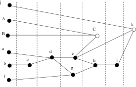
Figure 2: The dependency graph for the standard $\mathop{\wedge}\hskip-1.72218ptU$ pattern.

7 The no dependency theorems

From standardization we can also infer results related to dependencies. We start with a simple observation which is a direct consequence of standardization.

Lemma 14

Let $\mathcal{P}$ be a pattern implementing some cptp-maps $T$, and suppose $\mathcal{P}$’s command sequence has measurements only of the $M^{x}$ and $M^{y}$ kind, then $U$ has a standard implementation, having only independent measurements, all being of the $M^{x}$ and $M^{y}$ kind (therefore of computational depth complexity at most 2).

Proof. Write $\mathcal{P}^{\prime}$ for the standard pattern associated to $\mathcal{P}$. By equations (15) and (16), the $X$-actions can be eliminated from $\mathcal{P}^{\prime}$, and then $Z$-actions can be eliminated by using the extended calculus. The final pattern still implements $T$, has no longer any dependent measurements, and has therefore computational depth complexity at most 2. $\Box$

Theorem 4

Let $U$ be a unitary operator, then $U$ is in the Clifford group iff there exists a pattern $\mathcal{P}$ implementing $U$, having measurements only of the $M^{x}$ and $M^{y}$ kind.

Proof. The “only if” direction is easy, since we have seen in the example section, standard patterns for $\mathop{\wedge}\hskip-1.72218ptX$, $H$ and $P(\frac{\pi}{2})$ which had only independent $M^{x}$ and $M^{y}$ measurements. Hence any Clifford operator can be implemented by a combination of these patterns. By the lemma above, we know we can actually choose these patterns to be standard.

For the “if” direction, we prove that $U$ belongs to the normalizer of the Pauli group, and hence by definition to the Clifford group. In order to do so we use the standard form of $\mathcal{P}$ written as $\mathcal{P}^{\prime}=C_{\mathcal{P}^{\prime}}M_{\mathcal{P}^{\prime}}E_{\mathcal{P}^{\prime}}$ which still implements $U$, and has only $M^{x}$ and $M^{y}$ measurements. Recall that, because of equations (15) and (16), these measurements are independent.

Let $i$ be an input qubit, and consider the pattern $\mathcal{P}^{\prime\prime}={\mathcal{P}}^{\prime}C_{i}$, where $C_{i}$ is either $X_{i}$ or $Z_{i}$. Clearly $\mathcal{P}^{\prime\prime}$ implements $UC_{i}$. First, one has:

$$\begin{array}[c]{lllllllllllllll}C_{\mathcal{P}^{\prime}}M_{\mathcal{P}^{\prime}}E_{\mathcal{P}^{\prime}}C_{i}&\Rightarrow_{EC}^{\star}&C_{\mathcal{P}^{\prime}}M_{\mathcal{P}^{\prime}}C^{\prime}E_{\mathcal{P}^{\prime}}\end{array}$$

for some non-dependent sequence of corrections $C^{\prime}$, which, up to free commutations can be written uniquely as $C^{\prime}_{O}C^{\prime\prime}$, where $C^{\prime}_{O}$ applies on output qubits, and therefore commutes to $M_{\mathcal{P}^{\prime}}$, and $C^{\prime\prime}$ applies on non-output qubits (which are therefore all measured in $M_{\mathcal{P}^{\prime}}$). So, by commuting $C^{\prime}_{O}$ both through $M_{\mathcal{P}^{\prime}}$ and $C_{\mathcal{P}^{\prime}}$ (up to a global phase), one gets:

$$\begin{array}[c]{lllllllllllllll}C_{\mathcal{P}^{\prime}}M_{\mathcal{P}^{\prime}}C^{\prime}E_{\mathcal{P}^{\prime}}&\Rightarrow^{\star}&C^{\prime}_{O}C_{\mathcal{P}^{\prime}}M_{\mathcal{P}^{\prime}}C^{\prime\prime}E_{\mathcal{P}^{\prime}}\end{array}$$

Using equations (15), (16), and the extended calculus to eliminate the remaining $Z$-actions, one gets:

$$\begin{array}[c]{lllllllllllllll}M_{\mathcal{P}^{\prime}}C^{\prime\prime}&\Rightarrow_{MC,S}^{\star}&SM_{\mathcal{P}^{\prime}}\end{array}$$

for some product $S=\prod_{\{j\in J\}}S_{j}^{1}$ of constant shifts , applying to some subset $J$ of the non-output qubits. So:

$$\begin{array}[c]{lllllllllllllll}C^{\prime}_{O}C_{\mathcal{P}^{\prime}}M_{\mathcal{P}^{\prime}}C^{\prime\prime}E_{\mathcal{P}^{\prime}}&\Rightarrow^{\star}_{MC,S}&C^{\prime}_{O}C_{\mathcal{P}^{\prime}}SM_{\mathcal{P}^{\prime}}E_{\mathcal{P}^{\prime}}\\ &\Rightarrow^{\star}&C^{\prime}_{O}C^{\prime\prime}_{O}C_{\mathcal{P}^{\prime}}M_{\mathcal{P}^{\prime}}E_{\mathcal{P}^{\prime}}\end{array}$$

where $C^{\prime\prime}_{O}$ is a further constant correction obtained by signal shifting $C_{\mathcal{P}^{\prime}}$ with $S$. This proves that $\mathcal{P}^{\prime\prime}$ also implements $C^{\prime}_{O}C^{\prime\prime}_{O}U$, and therefore $UC_{i}=C^{\prime}_{O}C^{\prime\prime}_{O}U$ which completes the proof, since $C^{\prime}_{O}C^{\prime\prime}_{O}$ is a non dependent correction. $\Box$

The “only if” part of this theorem already appears in previous work [RBB03, p.18]. The “if” part can be construed as an internalization of the argument implicit in the proof of Gottesman-Knill theorem [NC00, p.464].

We can further prove that dependencies are crucial for the universality of the model. Observe first that if a pattern has no measurements, and hence no dependencies, then it follows from (D2) that $V=O$, i.e., all qubits are outputs. Therefore computation steps involve only $X$, $Z$ and $\mathop{\wedge}\hskip-1.72218ptZ$, and it is not surprising that they compute a unitary which is in the Clifford group. The general argument essentially consists in showing that when there are measurements, but still no dependencies, then the measurements are playing no part in the result.

Theorem 5

Let $\mathcal{P}$ be a pattern implementing some unitary $U$, and suppose $\mathcal{P}$’s command sequence doesn’t have any dependencies, then $U$ is in the Clifford group.

Proof. Write $\mathcal{P}^{\prime}$ for the standard pattern associated to $\mathcal{P}$. Since rewriting is sound, $\mathcal{P}^{\prime}$ still implements $U$, and since rewriting never creates any dependency, it still has no dependencies. In particular, the corrections one finds at the end of $\mathcal{P}^{\prime}$, call them $C$, bear no dependencies. Erasing them off $\mathcal{P}^{\prime}$, results in a pattern $\mathcal{P}^{\prime\prime}$ which is still standard, still deterministic, and implementing $U^{\prime}:=C^{\dagger}U$.

Now how does the pattern $\mathcal{P}^{\prime\prime}$ run on some input $\phi$ ? First $\phi\otimes{|}\hskip-1.72218pt+\ldots+\rangle$ goes by the entanglement phase to some $\psi\in\mathfrak{H}_{V}$, and is then subjected to a sequence of independent 1-qubit measurements. Pick a basis $\mathbf{B}$ spanning the Hilbert space generated by the non-output qubits $\mathfrak{H}_{V\smallsetminus O}$ and associated to this sequence of measurements.

Since $\mathfrak{H}_{V}=\mathfrak{H}_{O}\otimes\mathfrak{H}_{V\smallsetminus O}$ and $\mathfrak{H}_{V\smallsetminus O}=\oplus_{\phi_{b}\in\mathcal{B}}[\phi_{b}]$, where $[\phi_{b}]$ is the linear subspace generated by $\phi_{b}$, by distributivity, $\psi$ uniquely decomposes as:

$$\begin{array}[c]{lllllllllllllll}\psi=\sum_{\phi_{b}\in\mathcal{B}}x_{b}\otimes\phi_{b}\end{array}$$

where $\phi_{b}$ ranges over $\mathcal{B}$, and $x_{b}\in\mathfrak{H}_{O}$. Now since $\mathcal{P}^{\prime\prime}$ is deterministic, there exists an $x$, and scalars $\lambda_{b}$ such that $x_{b}=\lambda_{b}x$. Therefore $\psi$ can be written $x\otimes\psi^{\prime}$, for some $\psi^{\prime}$. It follows in particular that the output of the computation will still be $x$ (up to a scalar), no matter what the actual measurements are. One can therefore choose them to be all of the ${M}^{x}$ kind, and by the preceding theorem $U^{\prime}$ is in the Clifford group, and so is $U=CU^{\prime}$, since $C$ is a Pauli operator. $\Box$

From this section, we conclude in particular that any universal set of patterns has to include dependencies (by the preceding theorem), and also needs to use measurements $M^{\alpha}$ where $\alpha\neq 0$ modulo $\frac{\pi}{2}$ (by the theorem before). This is indeed the case for the universal set $\mathcal{J}(\alpha)$ and $\mathop{\wedge}\hskip-1.72218pt{\mathcal{Z}}$.

8 Other Models

There are several other approaches to measurement-based computation as we have mentioned in the introduction. However, it is only for the one-way model that the importance of having all the entanglement in front has been emphasized. For example, Gottesman and Chuang describe computing with teleportation in the setting of the circuit model and hence the computation is very sequential [GC99]. What we will do is to give a general treatment of a variety of measurement-based models – including some that appear here for the first time – in the setting of our calculus. More precisely we would like to know other potential definitions for commands $N$, $E$, $M$ and $C$ that lead to a model that still satisfies the properties of: (i) being closed under composition; (ii) universality and (iii) standardization.

Moreover we are interested in obtaining a compositional embedding of these models into a single one-qubit measurement-based model. The teleportation model can indeed be embedded into the one-way model. There is, however, a new model, the Pauli model – formally defined here for the first time – which is motivated by considerations of fault tolerance [RAB04, DK05b, DKOS06]. The Pauli model can be embedded into a slight generalization of the one-way model called the phase model; also given here for the first time. The one-way model will trivially embed in the phase model so by composition all the measurement-based models will embed in the phase model. We could have done everything ab initio in terms of the phase model but this would have made much of the presentation unnecessarily complicated at the outset.

We recall the remark from the introduction that these embeddings have three advantages: first, we get a workable syntax for handling the dependencies of operators on previous measurement outcomes, second, one can use these embeddings to transfer the measurement calculus previously developed for the one-way model to obtain a calculus for the new model including, of course, a standardization procedure that we get automatically; lastly, one can embed the patterns from the phase model into the new models and vice versa. In essence, these compositional embeddings will allow us to exhibit the phase model as being a core calculus for measurement-based computation. However different models are interesting from the point of view of implementation issues like fault-tolerance and ease of preparation of entanglement resources. Our embeddings allow one to move easily between these models and to concentrate on the one-way model for designing algorithms and proving general theorems.

This section has been structured into several subsections, one for each model and its embedding.

8.1 Phase Model

In the one-way model the auxiliary qubits are initialized to be in the ${|}+\rangle$ state. We extend the one-way model to allow the auxiliary qubits to be in a more general state. We define the extended preparation command $N^{\alpha}_{i}$ to be the preparation of the auxiliary qubit $i$ in the state ${|}+_{\alpha}\rangle$. We also add a new correction command $Z^{\alpha}_{i}$, called a phase correction to guarantee that we can obtain determinate patterns. The dependent phase correction is written as $Z_{i}^{\alpha,s}$ with $Z_{i}^{\alpha,0}=I$ and $Z_{i}^{\alpha,1}=\left(\begin{matrix}1&0\\ 0&e^{i\alpha}\end{matrix}\right)$. Under conjugation, the phase correction, defines a new action over measurement:

$$\begin{array}[c]{lllllllllllllll}(Z_{i}^{\beta,s}){}^{{\dagger}}{M}_{i}^{{\alpha}}Z_{i}^{\beta,s}={M}_{i}^{\alpha-s\beta}\end{array}$$

and since the measurement is destructive, it simplifies to ${M}_{i}^{\alpha}Z_{i}^{\beta,s}={M}_{i}^{\alpha-s\beta}$. This action does not commute with Pauli actions and hence one cannot write a compact notation for dependent measurement, as we did before, and the computation of angle dependencies is a bit more complicated. Thereafter, a measurement preceded by a sequence of corrections on the same qubit will be called a dependent measurement. Note that, by the absorption equations, this indeed can be seen as a measurement, where the angle depends on the outcomes of some other measurements made beforehand.

To complete the extended calculus it remains to define the new rewrite rules:

$$\begin{array}[c]{lllllllllllllll}E_{ij}Z_{i}^{\alpha,s}&\Rightarrow&Z_{i}^{\alpha,s}E_{ij}&\quad\hbox{}EP\\ \\ {M}_{i}^{\alpha}X_{i}^{s}&\Rightarrow&{M}_{i}^{(-1)^{s}\alpha}&\quad\hbox{}MX\\ {M}_{i}^{\alpha}Z_{i}^{s}&\Rightarrow&{M}_{i}^{\alpha-s\pi}&\quad\hbox{}MZ\\ {M}_{i}^{\alpha}Z_{i}^{\beta,s}&\Rightarrow&{M}_{i}^{\alpha-s\beta}&\quad\hbox{}MP\end{array}$$

The above rules together with the rewriting rules of the one-way model described in Section 5, lead to a standardization procedure for the model. It is trivial that the one-way model is a fragment of this generalized model and hence universality immediately follows. It is also easy to check that the model is closed under composition and all the semantical properties of the one-way model can be extended to this general model as well.

The choice of extended preparations and its concomitant phase correction is actually quite delicate. One wishes to keep the standardizability of the calculus which constrains what can be added but one also wishes to have determinate patterns which forces us to put in appropriate corrections. The phase model is only a slight extension of the original one-way model, but it allows a discussion of the next model which is of great physical interest.

8.1.1 Pauli model

An interesting fragment of the phase model is defined by restricting the angles of measurements to $\{0,\frac{\pi}{2},\pi,-\frac{\pi}{2}\}$ i.e.  Pauli measurements and the angles of preparation to $0$ and $\frac{\pi}{4}$. Also the correction commands are restricted to Pauli corrections $X$, $Z$ and Phase correction $Z^{\frac{\pi}{8}}$. One readily sees that the subset of angles is closed under the actions of the corrections and hence the Pauli model is closed under composition.

Proposition 15

The Pauli model is approximately universal.

Proof. We know that the set consisting of $J(0)$ (which is $H$), $J({\frac{\pi}{4}})$, and $\mathop{\wedge}\hskip-1.72218ptZ$ is approximately universal. Hence, to prove the approximate universality of Pauli model, it is enough to exhibit a pattern in the Pauli model for each of these three unitaries. We saw before that $J(0)$ and $\mathop{\wedge}\hskip-1.72218ptZ$ are computed by the following 2-qubit patterns:

$$\begin{array}[c]{lllllllllllllll}\mathcal{J}(0)&:=&X_{2}^{s_{1}}{M}_{1}^{0}E_{12}\\ \mathop{\wedge}\hskip-1.72218pt{\mathcal{Z}}&:=&E_{12}\end{array}$$

where both belong also to the Pauli model. The pattern for $J_{\frac{\pi}{4}}$ in the one-way model is expressed as follows:

$$\begin{array}[c]{lllllllllllllll}\mathcal{J}({\frac{\pi}{4}})&:=&X_{2}^{s_{1}}{M}_{1}^{-\frac{\pi}{4}}E_{12}\\ &=&X_{2}^{s_{1}}{M}_{1}^{0}E_{12}Z^{\frac{\pi}{4}}_{1}\end{array}$$

The above forms do not fit in the Pauli model, since the first one uses a measurement with an angle $\frac{\pi}{4}$ and the second uses $Z^{\frac{\pi}{4}}$. However by teleporting the input qubit and then applying the $Z^{\frac{\pi}{4}}$ and finally running the standardization procedure we obtain the following pattern in the Pauli model for $J(\frac{\pi}{4})$:

$$\begin{array}[c]{lllllllllllllll}&&X_{2}^{s_{1}}{M}_{1}^{0}E_{12}Z^{\frac{\pi}{4}}_{1}\\ &=&X_{4}^{s_{3}}{M}_{3}^{0}E_{34}\framebox{$Z^{\frac{\pi}{4}}_{3}$}Z_{3}^{s_{2}}X_{3}^{s_{1}}{M}_{2}^{0}{M}_{1}^{0}E_{12}E_{23}\\ &=&X_{4}^{s_{3}}{M}_{3}^{0}E_{34}Z_{3}^{s_{2}}Z_{3}^{\frac{\pi}{2},s_{2}}X_{3}^{s_{1}}{M}_{2}^{0}{M}_{1}^{0}E_{12}E_{23}\framebox{$Z^{\frac{\pi}{4}}_{3}$}\\ &=&X_{4}^{s_{3}}{M}_{3}^{0}E_{34}Z_{3}^{s_{2}}Z_{3}^{\frac{\pi}{2},s_{2}}X_{3}^{s_{1}}{M}_{2}^{0}{M}_{1}^{0}E_{12}E_{23}\framebox{$Z^{\frac{\pi}{4}}_{3}$}\\ &=&X_{4}^{s_{3}+s_{2}}Z_{4}^{s_{1}}{M}_{3}^{-(-1)^{s_{1}}{s_{2}}\frac{\pi}{2}}{M}_{2}^{0}{M}_{1}^{0}E_{12}E_{23}E_{34}N_{3}^{\frac{\pi}{4}}\end{array}$$

Approximate universality for the Pauli model is now immediate. $\Box$

Note that we cannot really expect universality (as we had for the phase model) because the angles are restricted to a discrete set. On the other hand it is precisely this restriction that makes the Pauli model interesting from the point of view of implementation. The other particular interest behind this model, apart from its simple structure, is based on the existence of a novel fault tolerant technique for computing within this framework [BK05, RAB04, DKOS06].

8.2 Teleportation

Another class of measurement-based models – older, in fact, than the one-way model – uses $2$-qubit measurements. These are collectively referred to as teleportation models [Leu04]. Several papers that are concerned with the relation and possible unification of these models [CLN05, AL04, JP05] have already appeared. One aspect of these models that stands in the way of a complete understanding of this relation, is that, whereas in the one-way model one has a clearly identified class of measurements, there is less agreement concerning which measurements are allowed in teleportation models.

We propose here to take as our class of $2$-qubit measurements a family obtained as the conjugate under the operator $\mathop{\wedge}\hskip-1.72218ptZ$ of tensors of $1$-qubit measurements. We show that the resulting teleportation model is universal. Moreover, almost by construction, it embeds into the one-way model, and thus exposes completely the relation between the two models.

Before embarking on the specifics of our family of $2$-qubit measurements, we remark that the situation commented above is more general:

Lemma 16

Let $\cal{A}$ be an orthonormal basis in $\otimes^{n}{\mathbb{C}}^{2}$, with associated $n$-qubit measurement $M^{\mathcal{A}}$, and $\mathcal{A}_{i}$ with $i=1,\ldots,n$ be orthonormal bases in ${\mathbb{C}}^{2}$, with associated $1$-qubit measurements $M^{\mathcal{A}_{i}}_{i}$. Then there exists a unique (up to a permutation) $n$-qubit unitary operator $U$ such that:

$$\begin{array}[c]{lllllllllllllll}M^{\mathcal{A}}_{1\cdots n}&=&U_{1\cdots n}(\otimes_{i}M^{\mathcal{A}_{i}}_{i})U^{\star}_{1\cdots n}\end{array}$$

Proof. Take $U$ to map $\otimes_{i}\mathcal{A}_{i}$ to $\mathcal{A}$. $\Box$

This simple lemma says that general $n$-qubit measurements can always be seen as conjugated $1$-qubit measurements, provided one uses the appropriate unitary to do so. As an example consider the orthogonal graph basis $\mathcal{G}=\mathop{\wedge}\hskip-1.72218ptZ_{12}\{{|}\pm\rangle\otimes{|}\pm\rangle\}$ then the two-qubit graph basis measurements are defined as $M^{\mathcal{G}}_{12}=\mathop{\wedge}\hskip-1.72218ptZ_{12}({M}_{1}^{0}\otimes{M}_{2}^{0})\mathop{\wedge}\hskip-1.72218ptZ_{12}$. It is now natural to extend our definition of $M^{\mathcal{G}}_{12}$ to obtain the family of $2$-qubit measurements of interest:

$$M_{12}^{\alpha,\beta} := \mathop{\wedge}\hskip-1.72218ptZ_{12}({M}_{1}^{\alpha}\otimes{M}_{2}^{\beta})\mathop{\wedge}\hskip-1.72218ptZ_{12}$$ (17)

corresponding to projections on the basis $\mathcal{G}_{\alpha,\beta}:=\mathop{\wedge}\hskip-1.72218ptZ_{12}(P_{1}(\alpha)\otimes P_{2}(\beta))(\{{|}\pm\rangle\otimes{|}\pm\rangle\}$. This family of two-qubit measurements together with the preparation, entanglement and corrections commands of the one-way model define the teleportation model.

Before we carry on, a clarification about our choice of measurements in the teleportation model is necessary. The usual teleportation protocol uses Bell basis measurement defined with

$$\begin{array}[c]{lllllllllllllll}\mathcal{B}&=&\mathop{\wedge}\hskip-1.72218ptX_{12}\{{|}\pm\rangle\otimes{|}0/1\rangle\}\\ M^{\mathcal{B}}_{12}&=&\mathop{\wedge}\hskip-1.72218ptX_{12}({M}_{1}^{z}\otimes{M}_{2}^{z})\mathop{\wedge}\hskip-1.72218ptX_{12}\end{array}$$

where $M^{z}$ is the computational-basis measurement. Note how similar these equations are to the equations defining the graph basis measurements. This is a clear indication that everything that follows can be transferred to the case where $X$ replaces $Z$, and $\mathcal{B}$ replaces $\mathcal{G}$. However, since the methodology we adopt is to embed the 2-qubit measurement based model in the one-way model, and the latter is based on $\mathop{\wedge}\hskip-1.72218ptZ$ and $\mathcal{G}$, we will work with the graph-basis measurements. Furthermore, since $\mathop{\wedge}\hskip-1.72218ptZ$ is symmetric, whereas $\mathop{\wedge}\hskip-1.72218ptX$ (a.k.a. as C-NOT) is not, the algebra is usually nicer to work with.

Now we prove that the family of measurements in Equation 17 leads to a universal model, which embeds nicely into the one-way model, but first we need to describe the important notion of dependent measurements. These will arise as a consequence of standardization; they were not considered in the existing teleportation models.

In what follows we drop the subscripts on the $\mathop{\wedge}\hskip-1.72218ptZ$ unless they are really necessary. We write $(s(i),s(j))\in{\mathbb{Z}}_{2}\times{\mathbb{Z}}_{2}$ to represent outcome of a 2-qubit measurement, with the specific convention that $(0,0)$, $(0,1)$, $(1,0)$, and $(1,1)$, correspond respectively to the cases where the state collapses to $\mathop{\wedge}\hskip-1.72218ptZ{|}+_{\alpha}\rangle{|}+_{\alpha}\rangle$, $\mathop{\wedge}\hskip-1.72218ptZ{|}+_{\alpha}\rangle{|}-_{\alpha}\rangle$, $\mathop{\wedge}\hskip-1.72218ptZ{|}-_{\alpha}\rangle{|}+_{\alpha}\rangle$, and $\mathop{\wedge}\hskip-1.72218ptZ{|}-_{\alpha}\rangle{|}-_{\alpha}\rangle$.

We will use two types of dependencies for measurements associated with $X$-action and $Z$-action:

$$\begin{array}[c]{lllllllllllllll}[{M}_{ij}^{\alpha,\beta}]^{(s,t)}&=&M_{ij}^{(-1)^{s}\alpha,(-1)^{t}\beta}\\ {}^{(u,v)}[{M}_{ij}^{\alpha,\beta}]&=&M_{ij}^{\alpha+u\pi,\beta+v\pi}\end{array}$$

where $s$, $t$, $u$ and $v$ are in ${\mathbb{Z}}_{2}$. The two actions commute, so the equations above define unambiguously the full dependent measurement ${}^{(u,v)}[{M}_{ij}^{\alpha,\beta}]^{(s,t)}$. Here are some useful abbreviations:

$$\begin{array}[c]{lllllllllllllll}{}^{(0,0)}[{M}^{\alpha,\beta}]^{(s,t)}:=[{M}^{\alpha,\beta}]^{(s,t)}\\ {}^{(u,v)}[{M}^{\alpha,\beta}]^{(0,0)}:={}^{(u,v)}[{M}^{\alpha,\beta}]\\ {}^{(0,0)}[{M}^{\alpha,\beta}]^{(0,0)}:=M^{\alpha,\beta}\\ M^{\alpha,x}:=M^{\alpha,0}\\ M^{\alpha,y}:=M^{\alpha,\frac{\pi}{2}}\\ \end{array}$$

As in the 1-qubit measurement case we obtain the following rewriting rules for the teleportation model:

$$\begin{array}[c]{lllllllllllllll}E_{ij}X_{i}^{s}&\Rightarrow&X_{i}^{s}Z_{j}^{s}E_{ij}&\quad\hbox{}EX\\ E_{ij}Z_{i}^{s}&\Rightarrow&Z_{i}^{s}E_{ij}&\quad\hbox{}EZ\\ {}^{(u,v)}[{M}_{ij}^{\alpha,\beta}]^{(s,t)}X_{i}^{r}&\Rightarrow&{}^{(u,v+r)}[{M}_{ij}^{\alpha,\beta}]^{(s+r,t)}&\quad\hbox{}MX\\ {}^{(u,v)}[{M}_{ij}^{\alpha,\beta}]^{(s,t)}X_{j}^{r}&\Rightarrow&{}^{(u+r,v)}[{M}_{ij}^{\alpha,\beta}]^{(s,t+r)}&\quad\hbox{}MX\\ {}^{(u,v)}[{M}_{ij}^{\alpha,\beta}]^{(s,t)}Z_{i}^{r}&\Rightarrow&{}^{(u+r,v)}[{M}_{ij}^{\alpha,\beta}]^{(s,t)}&\quad\hbox{}MZ\\ {}^{(u,v)}[{M}_{ij}^{\alpha,\beta}]^{(s,t)}Z_{j}^{r}&\Rightarrow&{}^{(u,v+r)}[{M}_{ij}^{\alpha,\beta}]^{(s,t)}&\quad\hbox{}MZ\end{array}$$

to which we add also the trivial commutation rewriting which are possible between commands that don’t overlap (meaning, acting on disjoint sets of qubits).

8.2.1 Embedding

We describe how to translate $2$-qubit EMC patterns to $1$-qubit patterns and vice versa. The following equation plays the central role in the translation:

$$M_{ij}^{\alpha,\beta}=E_{ij}({M}_{i}^{\alpha}\otimes{M}_{j}^{\beta})E_{ij}$$ (18)

Note that this immediately gives the denotational semantics of two-qubit measurements as cptp-maps. Furthermore, all other commands in the teleportation model are the same as in the one-way model, so we have right away a denotational semantics for the entire teleportation model in terms of cptp-maps.

We write $\mathfrak{P}$ for the collection of patterns in the one-way model and $\mathfrak{T}$ for the collection of patterns in the teleportation model.

Theorem 6

There exist functions $[\cdot]_{f}:\mathcal{P}\to\mathcal{T}$ and $[\cdot]_{b}:\mathcal{T}\to\mathcal{P}$ such that

1. $\forall\mathcal{P}\in\mathfrak{P}:[[\mathcal{P}]]=[[[\mathcal{P}]_{f}]]$;

2. $\forall\mathcal{T}\in\mathfrak{T}:[[\mathcal{T}]]=[[[\mathcal{T}]_{b}]]$;

3. $[\cdot]_{f}\circ[\cdot]_{b}$ and $[\cdot]_{b}\circ[\cdot]_{f}$ are both identity maps.

Proof. We first define the forward map $[\cdot]_{f}$ in stages as follows for any patterns $\mathcal{P}=(V,I,O,A_{n}\ldots A_{1})$:

1. For any $i\in V\smallsetminus O$ (i.e. measured qubits) we add an auxiliary qubit $i_{d}$ called a dummy qubit to the space $V$.

2. For any $i\in V\smallsetminus O$ we replace any occurrence of $M_{i}^{\alpha}$ with $M_{i}^{\alpha}M_{i_{d}}^{x}$ .

3. We then replace each of the newly created occurrences of $M_{i}^{\alpha}M_{i_{d}}^{x}$ by $M_{ii_{d}}^{\alpha,x}E_{ii_{d}}$ .

Now we show that the first condition stated in the theorem holds; we do this stage wise. The first two stages are clear because we are just adding qubits that have no effect on the pattern because they are not entangled with any pre-existing qubit, and no other command depends on a measurement applied to one of the dummy qubits. Furthermore, we add qubits in the state ${|}+\rangle$ and measure them in the ${|}\pm\rangle$ basis. The invariance of the semantics under stage 3 is an immediate consequence of Equation 18 and the fact that all the measurements are destructive, and hence an entanglement command on qubits appearing after a measurement of any of those qubits can just be removed.

The map $[\cdot]_{b}$ is defined similarly except that there is no need to add dummy qubits. One only needs to replace any two-qubit measurement $M^{\alpha,\beta}_{ij}$ with $M_{i}^{\alpha}M_{j}^{\beta}E_{ij}$. Again, this clearly preserves the semantics of patterns because of Equation 18 and the above remark about destructive measurements. Thus condition 2 of the theorem holds.

The fact that the two maps are mutual inverses follows easily. As all the steps in the translations are local we can reason locally. Looking at the forward mapping followed by the backward mapping we get the following sequence of transformations

$$\begin{array}[c]{lllllllllllllll}M_{i}^{\alpha}&\Rightarrow_{\text{stage }1,2}&M_{i}^{\alpha}M_{i_{d}}^{x}\\ &\Rightarrow_{\text{Equation \ref{s2to1m}}}&M_{ii_{d}}^{\alpha,x}E_{ii_{d}}\\ &\Rightarrow_{\text{Equation \ref{s2to1m}}}&M_{i}^{\alpha}M_{i_{d}}^{x}E_{ii_{d}}E_{ii_{d}}\\ &\Rightarrow&M_{i}^{\alpha}M_{i_{d}}^{x}\\ &\Rightarrow&M_{i}^{\alpha}\end{array}$$

This shows that we have the third condition of the theorem. $\Box$

Note that the translations are compositional since the denotational semantics is and also it follows immediately that the teleportation model is universal and admits a standardization procedure.

Example. Consider the teleportation pattern in the teleportation model given by the command sequence: $X_{3}^{s_{1}}Z_{3}^{s_{2}}M_{12}^{x,x}E_{23}$, we perform the above steps:

$$\begin{array}[c]{lllllllllllllll}X_{3}^{s_{1}}Z_{3}^{s_{2}}\framebox{$M_{12}^{x,x}$}E_{23}&\Rightarrow_{\text{Equation \ref{s2to1m}}}&\\ X_{3}^{s_{1}}Z_{3}^{s_{2}}{M}_{1}^{x}{M}_{2}^{x}E_{12}E_{23}\end{array}$$

and hence obtain the teleportation pattern with $1$-qubit measurements.

Example. We saw before, the following EMC $1$-qubit pattern for $R_{z}(\alpha)$ which can be embedded to an EMC $2$-qubit pattern using the above steps:

$$\begin{array}[c]{lllllllllllllll}X_{3}^{s_{2}}Z_{3}^{s_{1}}\framebox{$[{M}_{2}^{x}]^{s_{1}}{M}_{1}^{-\alpha}$}E_{12}E_{23}&\Rightarrow_{\text{stage 1,2}}&\\ X_{3}^{s_{2}}Z_{3}^{s_{1}}\framebox{$[{M}_{2}^{x}]^{s_{1}}{M}_{2_{d}}^{x}{M}_{1}^{-\alpha}{M}_{1_{d}}^{x}$}E_{12}E_{23}&\Rightarrow_{\text{Equation \ref{s2to1m} and standardization}}&\\ X_{3}^{s_{2}}Z_{3}^{s_{1}}[{M}_{22_{d}}^{x,x}]^{(s_{1},0)}M_{11_{d}}^{-\alpha,x}E_{11_{d}}E_{22_{d}}E_{12}E_{23}\end{array}$$

Note that we have explicit algorithmic translations between the models and not just illustrative examples. This is the main advantage of our approach in unifying these two models compared to the extant work [CLN05, AL04, JP05].

9 Conclusion

We have presented a calculus for the one-way quantum computer. We have developed a syntax of patterns and, much more important, an algebra of pattern composition. We have seen that pattern composition allows for a structured proof of universality, which also results in parsimonious implementations. We develop an operational and denotational semantics for this model; in this simple first-order setting their equivalence is clear.

We have developed a rewrite system for patterns which preserves the semantics. We have shown further that our calculus defines a polynomial-time standardization algorithm transforming any pattern to a standard form where entanglement is done first, then measurements, then local corrections. We have inferred from this procedure that the denotational semantics of any pattern is a cptp-map and also proved that patterns with no dependencies, or using only Pauli measurements, may only implement unitaries in the Clifford group.

In addition we introduced some variations of the one-way and teleportation models and presented compositional back-and-forth embeddings of these models into the one-way model. This allows one to carry forward all the theory we have developed: semantics, rewrite rules, standardization, no-dependency theorems and universality. In fact the result of making the connection between the one-way model and the teleportation model is to introduce ideas: dependent measurements, standard forms for patterns and a standardization procedure which had never been considered before for the teleportation model. This shows the generality of our formalism: we expect that any yet to be discovered measurement-based computation frameworks can be treated in the same way.

Perhaps the most important aspect of standardization is the fact that now we can make patterns maximally parallel and distributed because all the entanglement operators, i.e.  non-local operators, can be performed at the beginning of the computation. Then from the dependency structure that can be obtained from the standard form of a pattern the measurements can be organized to be as parallel as possible. This is the essence of the difference between measurement-based computation and the quantum circuit model or the quantum Turing machine.

We feel that our measurement calculus has shown the power of the formalisms developed by the programming languages community to analyze quantum computations. The ideas that we use: rewriting theory, (primitive) type theory and above all, the importance of reasoning compositionally, locally and modularly, are standard for the analysis of traditional programming languages. However, for quantum computation these ideas are in their infancy. It is not merely a question of adapting syntax to the quantum setting; there are fundamental new ideas that need to be confronted. What we have done here is to develop such a theory in a new, physically-motivated setting.

There were prior discussions about putting patterns in a standard form [RB02] but these worked only with strongly deterministic patterns, furthermore one needs to know which unitary is being implemented. In our case the rewrite rules are entirely local and work equally well with all patterns.

An interesting question related to the measurement calculus is whether one can give sufficient conditions – depending only on the entanglement structure of a pattern – that guarantee determinacy. In a related paper the first two authors have solved this problem [DK05a]. In effect given an entanglement structure with distinguished inputs and outputs one can enumerate all the unitaries that can be implemented with it. This gives a precise handle on the entanglement resources needed in the design of specific algorithms and protocols directly in the measurement-based model [dBDK06].

Finally, there is also a compelling reading of dependencies as classical communications, while local corrections can be thought of as local quantum operations in a multipartite scenario. From this point of view, standardization pushes non-local operations to the beginning of a distributed computation, and it seems the measurement calculus could prove useful in the analysis of distributed quantum protocols. To push this idea further, one needs first to articulate a definition of a distributed version of the measurement calculus; this was done in a recent paper [DDKP05]. The distributed version of the calculus was then used to analyze a variety of quantum protocols and to examine the notion of knowledge flow in them [DP05].

Appendix A Background on Quantum Mechanics and Quantum Computation

We give a brief summary of quantum mechanics and quantum computing. We develop some of the algebra, define some notations, and prove a couple of equations which we have used in the paper. Although the paper is self-contained, the reader will find the expository book of Nielsen and Chuang [NC00] useful for quantum computation or the excellent book by Peres [Per95] for general background on quantum mechanics.

A.1 Linear Algebra for Quantum Mechanics

We assume that the reader is familiar with the basic notion of a vector space. In quantum mechanics we always consider vector spaces over the complex numbers. For quantum computation the vector spaces are always finite dimensional. The vector spaces that arise in quantum mechanics are Hilbert spaces and are thus usually written $\mathfrak{H}$; that is they have an inner product usually written $\langle u,v\rangle$ where $u$ and $v$ are vectors. The inner product is a map from $\mathfrak{H}\times\mathfrak{H}$ to the complex numbers $\mathbb{C}$. The inner product is linear in the second argument but anti-linear in the first argument. In general, there is a topological completeness condition on Hilbert spaces but, in the finite dimensional case this is automatic and we will ignore it.

Following Dirac, it is customary to call elements of $\mathfrak{H}$ kets and write them in the form ${|}u\rangle$ or whatever symbol is appropriate inside the half-bracket. The dual vectors are called bras and are written $\langle v{|}$; the pairing thus can naturally be identified – conceptually and notationally – with the inner product.

Linear operators come naturally with vector spaces; a linear operator is a linear map from a vector space to itself. Linear operators on finite dimensional spaces are often represented as matrices. The most important notion for an operator on a Hilbert space is that of an adjoint.

Definition 17

If $A:\mathfrak{H}\to\mathfrak{H}^{\prime}$ is a linear operator then the adjoint, written $A^{\dagger}$, is a linear operator from $\mathfrak{H}^{\prime}$ to $\mathfrak{H}$ such that

$$\forall u\in\mathfrak{H}^{\prime},v\in\mathfrak{H}\mbox{$\langle u,Av\rangle$}=\mbox{$\langle A^{\dagger}u,v\rangle$}.$$

In terms of matrices this just amounts to transposing the matrix and complex conjugation each of the matrix entries; sometimes this is called the hermitian conjugate. An inner product preserving linear map is called a unitary embedding. When $\mathfrak{H}=\mathfrak{H}^{\prime}$ we can also define the following operators. A hermitian operator $A$ is one such that $A=A^{\dagger}$ and a unitary operator $U$ is one such that $U^{-1}=U^{\dagger}$. A projection $P$ is a linear operator such that $P^{2}=P$ and $P=P^{\dagger}$. A projection operator can be identified with a subspace, namely its range. The eigenvalues of a hermitian operator are always real. Suppose $U$ is a unitary, and $P$ a projection, then $UPU^{\dagger}$ is also a projection.

It is common to use the Dirac notation to write projection operators as follows: given a vector ${|}a\rangle$ of unit norm, the projection onto the subspace spanned by ${|}a\rangle$ is written $|a\rangle\langle a|$. To see why this makes sense, suppose that ${|}b\rangle$ is another vector then its component along ${|}a\rangle$ is the inner product $\langle a,b\rangle$. Now if we just juxtapose the expressions $|a\rangle\langle a|$ and ${|}b\rangle$ we get ${|}a\rangle\mbox{$\langle a,b\rangle$}$, viewing the $\langle a,b\rangle$ as a number and moving it to the front we get $\mbox{$\langle a,b\rangle$}{|}a\rangle$ as the result, which is the right answer for the projection of ${|}b\rangle$ onto ${|}a\rangle$. Thus one can apply the projection operator just by juxtaposing it with the vector. This kind of suggestive manipulation is part of the appeal of the Dirac notation.

One important fact – the spectral theorem for hermitian operators – states that if $M$ is a hermitian operator, $\lambda_{i}$ are its eigenvalues and $P_{i}$ are projection operators onto the corresponding eigenspaces then one can write

$$M=\sum_{i}\lambda_{i}P_{i}.$$

If we have ${|}i\rangle$ as the normalized eigenvectors for the eigenvalues $\lambda_{i}$ then we can write this in Dirac notation as:

$$M=\sum_{i}\lambda_{i}|i\rangle\langle i|.$$

Finally we need to combine Hilbert spaces.

Definition 18

Given two Hilbert spaces $\mathfrak{H}$ with basis vectors $\{a_{i}|1\leq i\leq n\}$ and $\mathfrak{H}^{\prime}$ with basis $\{b_{j}|1\leq j\leq m\}$ we define the tensor product, written $\mathfrak{H}\otimes\mathfrak{H}^{\prime}$, as the vector space of dimension $n\cdot m$ with basis $a_{i}\otimes b_{j}$.

There are more elegant, basis-independent ways of describing the tensor product but this definition will serve our needs. We almost never write the symbol $\otimes$ between the vectors. In the Dirac notation this is always omitted and one writes, for example, ${|}uv\rangle$ instead of ${|}u\rangle\otimes{|}v\rangle$.

The important point is that there are vectors that cannot be written as the tensor product of vectors. For example, we can write $a_{1}\otimes b_{1}+a_{2}\otimes b_{2}$ where the $a_{i}$ and the $b_{i}$ are basis vectors of two $2$-dimensional Hilbert spaces. This means that given a general element of $\mathfrak{H}\otimes\mathfrak{H}^{\prime}$ one cannot produce elements of $\mathfrak{H}$ and $\mathfrak{H}^{\prime}$; this is very different from the cartesian product of sets. This is the mathematical manifestation of entanglement.

A very important function on square matrices is the trace. The usual trace – i.e. the sum of the diagonal entries – is basis independent and is actually equal to the sum of the eigenvalues, counted with multiplicity. The trace of $A$ is written $tr(A)$ and satisfies the cyclicity property $tr(AB)=tr(BA)$; applying this repeatedly one gets

$$tr(A_{1}\ldots A_{n})=tr(A_{\sigma(1)}\ldots A_{\sigma(n)})$$

where $\sigma$ is a cyclic permutation. The explicit formula for the trace of $A:V\to V$ is $tr(A)=\sum_{i}\langle i{|}A{|}i\rangle$ where ${|}i\rangle$ is a basis for $V$.

One often needs to compute a partial trace. Consider a linear map $L:V\otimes W\to V\otimes W$. Suppose that ${|}v_{i}\rangle$ is a basis for $V$ and ${|}w_{i}\rangle$ is a basis for $W$ then ${|}v_{i}w_{j}\rangle$ is a basis for $V\otimes W$. Now we can define the partial trace over $V$ as

$$tr_{V}(A):W\to W=\sum_{i}\langle v_{i}{|}A{|}v_{i}\rangle.$$

This corresponds to removing the $V$ dependency; often we use the phrase “tracing out the $V$ component.”

A.2 Quantum Mechanics

We state the basic facts of quantum mechanics and will not discuss the experimental basis for this framework. The key aspects of quantum mechanics are:

• the states of a quantum system form a Hilbert space,

• when two quantum systems are combined, the state space of the composite system is obtained as the tensor product of the state spaces of the individual systems, and

• the evolution of a quantum system is given by a unitary operator, and

• the effect of a measurement is indeterminate.

The first says that one can form superpositions of the states. This is one of the most striking features of quantum mechanics. Thus states are not completely distinct as they are in classical systems. The inner product measures the extent to which states are distinct. The fact that systems are combined by tensor product says that there are states that of composite systems that cannot be decomposed into individual pieces. This is the phenomenon of entanglement or non-locality.

Measurement is what gives quantum mechanics its indeterminate character. The usual case, called projective measurements, is when the quantity being measured is described by a hermitian operator $M$. The possible outcomes are the eigenvalues of $M$. If $M$ is an observable (hermitian operator) with eigenvalues $\lambda_{i}$ and eigenvectors ${|}\phi_{i}\rangle$ and we have a generic state ${|}\psi\rangle=\sum_{i}c_{i}{|}\phi_{i}\rangle$ then the probabilities and expectation values of the measurement outcomes are given by:

• $Prob(\lambda_{i}|{|}\psi\rangle)=|c_{i}|^{2}$

• $E[M|{|}\psi\rangle]=\sum_{i}|c_{i}|^{2}\lambda_{i}=\sum_{i}c_{i}\bar{c_{i}}\mbox{$\langle\phi_{i},M\phi_{i}\rangle$}=\mbox{$\langle\psi,M\psi\rangle$}.$

It is important to note that the effect of the measurement is that the projection operator $P_{i}$ is applied when the result $\lambda_{i}$ is observed. The operator $M$ does not describe the effect of the measurement.

The formulas above reveal that no aspect of a measurement is altered if the vector describing a quantum state is multiplied by a complex number of absolute value $1$. Thus we can multiply a state by $e^{i\theta}$ without changing the state. This is called changing the phase. While the phase is not important phase differences are very important. Multiplying a vector by a complex number is a change of phase as well as a change in its length. Usually we normalize the state so that we can read the results of measurements as probabilities. Given a vector the subspace spanned by it - always one dimensional – is called a ray. Thus a state is really a ray rather than a vector. However, it is customary to blur this distinction.

A.3 Some qubit algebra

Quantum computation is carried out with qubits the quantum analogues of bits. Just as a bit has two possible values, a qubit is a two dimensional complex Hilbert space, in other words it is (isomorphic to) the two dimensional complex vector space ${\mathbb{C}}^{2}$.

One works with a preferred basis, physically this corresponds to two distinguishable states, like “spin up” and “spin down”. One writes ${|}0\rangle$, and ${|}1\rangle$ for its canonical basis, so that any vector $\psi$ can be written as $\alpha{|}0\rangle+\beta{|}1\rangle$ with $\alpha$, $\beta$ in $\mathbb{C}$. Furthermore, ${\mathbb{C}}^{2}$ can be turned into a Hilbert space with the following inner product:

$$\begin{array}[c]{lllllllllllllll}\langle\alpha{|}0\rangle+\beta{|}1\rangle,\alpha^{\prime}{|}0\rangle+\beta^{\prime}{|}1\rangle\rangle&:=&\alpha^{\star}\alpha^{\prime}+\beta^{\star}\beta^{\prime}\end{array}$$

where $\alpha^{\star}$ is the complex conjugate of $\alpha$. One then obtains the norm of a vector as:

$$\begin{array}[c]{lllllllllllllll}\|\psi\|&:=&\langle\psi,\psi\rangle^{\frac{1}{2}}&=&(\alpha^{\star}\alpha+\beta^{\star}\beta)^{\frac{1}{2}}\end{array}$$

Given $V$ a finite set, one writes $\mathfrak{H}_{V}$ for the Hilbert space $\otimes_{u\in V}{\mathbb{C}}^{2}$; the notation means an $n$-fold tensor product of the ${\mathbb{C}}^{2}$ where $n$ is the size of $V$. A vector in $\mathfrak{H}_{V}$ is said to be decomposable if it can be written $\otimes_{u\in V}\psi_{u}$ for some $\psi_{u}\in{\mathbb{C}}^{2}$. Such decomposable vectors will be written $\epsilon$ in the sequel. Decomposable vectors can be represented by a map from $V$ to ${\mathbb{C}}^{2}$, and we will use both notations depending on which is more convenient. As we have noted before there are some vectors that are not decomposable.

As in the case of ${\mathbb{C}}^{2}$, there is a canonical basis for $\mathfrak{H}_{V}$, sometimes also called the computational basis, containing decomposable vectors $\epsilon$ such that for all $v\in V$, $\epsilon(v)={|}0\rangle$ or $\epsilon(v)={|}1\rangle$.

The inner product on $\mathfrak{H}_{V}$, according to the general definition given above, is defined on decomposable vectors as:

$$\begin{array}[c]{lllllllllllllll}\langle\epsilon,\epsilon^{\prime}\rangle&:=&\prod_{v\in V}\langle\epsilon(v),\epsilon^{\prime}(v)\rangle\end{array}$$

Note that all vectors in the computational basis are orthogonal and of norm $1$. The vectors of norm $1$ are usually called unit vectors; we always assume that states are described by unit vectors as noted before.

Here are some common states that arise in quantum computation:

$${|}0\rangle={|}\uparrow\rangle=\left[\begin{array}[]{c}1\\ 0\end{array}\right],{|}1\rangle={|}\downarrow\rangle=\left[\begin{array}[]{c}0\\ 1\end{array}\right],{|}+\rangle=\frac{1}{\sqrt{2}}\left[\begin{array}[]{c}1\\ 1\end{array}\right],{|}-\rangle=\frac{1}{\sqrt{2}}\left[\begin{array}[]{c}1\\ -1\end{array}\right].$$

It is easy to see that a linear operator is unitary if it preserves the inner product and hence the norm. Thus unitaries can be viewed as maps from quantum states to quantum states.

Some particularly useful unitaries are the Pauli operators given by the following matrices in the canonical basis of ${\mathbb{C}}^{2}$:

$$\begin{array}[c]{lllllllllllllll}X=\left(\begin{matrix}0&1\\ 1&0\end{matrix}\right),&Y=\left(\begin{matrix}0&{-i}\\ i&0\end{matrix}\right),&Z=\left(\begin{matrix}1&0\\ 0&{-1}\end{matrix}\right)\end{array}$$

We note that all these operators are involutive, self-adjoint, and therefore unitaries. All these matrices have determinant $=-1$. We will not discuss the geometric significance of these operators here; their real importance in quantum mechanics comes from the fact that they can be used to describe rotations, thus they are usually called the “Pauli spin matrices” by physicists.

Some basic algebra of these matrices are given below. First they all square to the identity.

$$X^{2}=Y^{2}=Z^{2}=I.$$

The Pauli operators do not commute. We use the notation $[A,B]$ for $AB-BA$, the commutator of $A$ and $B$. The commutator measures the extent to which two operators fail to commute: it is customary to present the algebra of operators using it. One also uses the symbol $\{A,B\}$ to stand for $AB+BA$: it is called the anti-commutator. For the Pauli operators we have the following commutators and anti-commutators :

	$XY=iZ$	$YX=-iZ$	$[X,Y]=2iZ$	$\{X,Y\}=0$
	$ZX=iY$	$XZ=-iY$	$[Z,X]=2iY$	$\{Z,X\}=0$
	$YZ=iX$	$ZY=-iX$	$[Y,Z]=2iX$	$\{Y,Z\}=0$

Definition 19

Define the Pauli group, $\mathbf{P}_{n}$, as the group consisting of tensor products of I, X, Y, and Z on n qubits, with an overall phase of $\pm 1$ or $\pm i$.

Given a group $G$ the operation $x\mapsto g^{-1}xg$ is called conjugation by $g$. These conjugations give the effect of switching operators around. If $G$ is a group and $H$ is a subgroup of $G$ then the normalizer of $H$ is another subgroup of $G$, say $K$, with the property that for all $h\in H,k\in K$ we have $k^{-1}hk$ in $H$.

The effect of conjugating measurements and other corrections by Pauli operators is a key part of the rewrite rules described in the main text. They can be verified using the algebra given here.

A very important related group is called the Clifford group.

Definition 20

The Clifford group, $\mathbf{C}_{n}$, is the group of unitary operators that leave the Pauli group invariant under conjugation, i.e. it is the normalizer of the Pauli group viewed as a subgroup of the unitary group.

The Clifford group on n qubits can be generated by the Hadamard transform, the controlled-$X$ ($CNOT$) or controlled-$Z$ ($\mathop{\wedge}\hskip-1.72218ptZ$), and the single-qubit phase rotation:

$$\begin{array}[c]{lllllllllllllll}H=\frac{1}{\sqrt{2}}\left(\begin{matrix}1&1\\ 1&-1\end{matrix}\right),&CNOT=\left(\begin{matrix}1&0&0&0\\ 0&1&0&0\\ 0&0&0&1\\ 0&0&1&0\end{matrix}\right),&\mathop{\wedge}\hskip-1.72218ptZ=\left(\begin{matrix}1&0&0&0\\ 0&1&0&0\\ 0&0&1&0\\ 0&0&0&-1\end{matrix}\right),&P=\left(\begin{matrix}1&0\\ 0&i\end{matrix}\right)\end{array}$$

The importance of the Clifford group for quantum computation is that a computation consisting of only Clifford operations on the computational basis followed by final Pauli measurements can be efficiently simulated by a classical computer, this is the Gottesman-Knill theorem [Got97, NC00].

A.4 Density Matrices

In order to capture partial information about quantum systems one uses density matrices. Before we describe density matrices we review some linear algebra in the bra-ket notation. Given a ket ${|}\psi\rangle$ the notation $|\psi\rangle\langle\psi|$ denotes the projection operator onto the one dimensional subspace spanned by ${|}\psi\rangle$. To verify this note that

$$(|\psi\rangle\langle\psi|)({|}\psi\rangle={|}\psi\rangle\|\psi\|={|}\psi\rangle$$

and

$$(|\psi\rangle\langle\psi|)({|}\phi\rangle)={|}\psi\rangle\langle\psi|\phi\rangle=\langle\psi|\phi\rangle{|}\psi\rangle.$$

If ${|}\psi_{i}\rangle$ is an orthonormal basis for $\mathfrak{H}$ the identity matrix is written $\sum_{i}|\psi_{i}\rangle\langle\psi_{i}|$. If $Q$ is a linear operator with eigenvalues $q_{i}$ and eigenvectors ${|}q_{i}\rangle$, which form an orthonormal basis for $\mathfrak{H}$, we can represent $Q$ as $\sum_{i}q_{i}|q_{i}\rangle\langle q_{i}|$. To see this, let ${|}\psi\rangle=\sum_{i}c_{i}{|}q_{i}\rangle$ then

$$Q{|}\psi\rangle=\sum_{i}c_{i}Q{|}q_{i}\rangle=\sum_{i}c_{i}q_{i}{|}q_{i}\rangle$$

now using our representation for $Q$ we calculate

$$Q{|}\psi\rangle=\sum_{i}q_{i}|q_{i}\rangle\langle q_{i}|({|}\psi\rangle)=\sum_{i,j}c_{j}q_{i}{|}q_{i}\rangle\langle q_{i}|q_{j}\rangle=\sum_{i}c_{i}q_{i}{|}q_{i}\rangle.$$

This is a version of the spectral theorem that we mentioned in the first subsection of this appendix.

A state (i.e. a ray in $\mathfrak{H}$) is called a pure state. If $a$ and $b$ are distinct eigenvalues of some observable $A$ with corresponding eigenvectors ${|}a\rangle$ and ${|}b\rangle$ it is perfectly possible to prepare a state of the form $\frac{1}{\sqrt{2}}({|}a\rangle+{|}b\rangle)$. A measurement of $A$ on such a state will yield either $a$ or $b$ each with probability $\frac{1}{2}$. However, it is also possible that a mixture is prepared. That is to say instead of a quantum superposition a classical stochastic mixture is prepared. In order to describe these we will use density matrices.

For a system in a pure state ${|}\psi\rangle$, the density matrix is just the projection operator $|\psi\rangle\langle\psi|$. If we have an observable $Q$ with eigenvalues $q_{i}$ – assumed nondegenerate for simplicity – then we can expand ${|}\psi\rangle$ in terms of the eigenvectors by

$${|}\psi\rangle=\sum_{i}c_{i}{|}q_{i}\rangle.$$

Now the probability of observing $q_{i}$ when measuring $Q$ in the state ${|}\psi\rangle$ is $|\langle q_{i}|\psi\rangle|^{2}$. Recalling that the identity is given by $I=\sum_{j}|q_{j}\rangle\langle q_{j}|$ we get that

$$Prob(q_{i},{|}\psi\rangle)=\sum_{j}\langle q_{i}|\psi\rangle\langle\psi|q_{j}\rangle\langle q_{j}|q_{i}\rangle$$

which after rearranging and using the definition of trace of an operator yields

$$Tr((|q_{i}\rangle\langle q_{i}|)(|\psi\rangle\langle\psi|)).$$

If as is typical we write $\rho_{\psi}$ for the density matrix and $P_{i}$ for the projection operator onto the subspace spanned by the eigenvector ${|}q_{i}\rangle$ we get

$$Prob(q_{i},{|}\psi\rangle)=Tr(P_{i}\rho).$$

It is an easy calculation to show that the expectation value for $Q$ in the state ${|}\psi\rangle$ is $Tr(Q\rho)$.

What if the state is not known completely? Suppose that we only know that a system is one of several possible states ${|}\psi_{1}\rangle,\ldots,{|}\psi_{k}\rangle$ with probabilities $p_{1},\ldots,p_{k}$ respectively. We define the density matrix for such a state to be

$$\rho=\sum_{i=1}^{k}p_{i}|\psi_{i}\rangle\langle\psi_{i}|.$$

The same formulas for the probability of observing a value $q_{i}$ , i.e. $Tr(P_{i}\rho)$ and for the expectation value of $Q$, i.e. $Tr(Q\rho)$ apply. One can check directly that a density matrix has the following two properties.

Proposition 21

An operator $\rho$ on $\mathfrak{H}$ is a density matrix if and only if

• $\rho$ has trace $1$ and

• $\rho$ is a positive operator, which means that it has only positive eigenvalues or, equivalently, that for any $x\in\mathfrak{H}$ we have $\mbox{$\langle x,\rho x\rangle$}\geq 0$.

Furthermore, if $\rho$ is a density operator, $Tr(\rho^{2})\leq 1$ with equality if and only if $\rho$ is a pure state (i.e. a projection operator).

Suppose that we have a density matrix $\rho$ describing a pure state of an $n+m$ dimensional system. Now suppose that an observer can only see the first $n$ dimensions. The density matrix $\xi$ describing what he can see is contained by taking the partial trace over the $m$ dimensions that the observer cannot see. Doing this gives, in general, a nonpure state. Similarly a complementary observer who sees only the $m$ dimensions would construct her density matrix $\sigma$ by taking the appropriate partial trace. Taking these traces loses information; in fact, one cannot reconstruct $\rho$ even from both $\xi$ and $\sigma$. Certainly the tensor product of $\xi$ and $\sigma$ does not give back $\rho$. This is due to the loss of the cross-correlation information that was encoded in $\rho$ but is not represented in either $\xi$ or $\sigma$.

The axioms of quantum mechanics are easily stated in the language of density matrices. For example, if evolution from time $t_{1}$ to time $t_{2}$ is described by the unitary transformation $U$ and $\rho$ is the density matrix for time $t_{1}$, then the evolved density matrix $\rho^{\prime}$ for time $t_{2}$ is given by the formula $\rho^{\prime}=U\rho U^{\dagger}$. Similarly, one can describe measurements represented by projective operators in terms of density matrices [NC00, Pre98]. Thus if a projector $P$ acts on a state ${|}\psi\rangle$ then the result is $P{|}\psi\rangle$; the resulting transofrmation of density matrices is $|\psi\rangle\langle\mapsto|P|\psi\rangle\langle P|$. For a general density matrix $\rho$ we have $\rho\mapsto P\rho P$, note that since $P$ is self-adjoint we do not have to write $P^{\dagger}$.

A.5 Operations on Density matrices

What are the legitimate “physical” transformations on density matrices? Density matrices are positive operators and they have trace either equal to $1$ if we insist on normalizing them or bounded by $1$. These properties muct be preserved by any transformations on them.

We need first to define what it means for a vector to be positive. Any vector space $V$ can be equipped with a notion of positivity.

Definition 22

A subset $C$ of $V$ is called a cone if

• $x\in C$ implies that for any positive $\alpha$, $\alpha x\in C$,

• $x,y\in C$ implies that $x+y\in C$ and

• $x$ and $-x$ both in $C$ means that $x=0$.

We can define $x\geq 0$ to mean $x\in C$ and $x\geq y$ to mean $x-y\in C$.

Definition 23

An ordered vector space is just a vector space equipped with a cone.

It is easy to check the following explicitly.

Proposition 24

The collection of positive operators in the vector space of linear operators forms a cone.

Now we can say what it means for a map to be a positive map.

Definition 25

Abstractly, $L:(V,\leq_{V})\to(W,\leq_{W})$ is a positive map if

$$\forall v\in V.\;\;v\geq_{V}0\Rightarrow L(v)\geq_{W}0.$$

It is important to not confuse “positive maps” and “positive operators.”

If we are transforming states (density matrices) then the legitimate transformations obviously take density matrices to density matrices. They have to be positive maps considered as maps between the appropriate ordered vector spaces. The appropriate ordered vector spaces are the vector spaces of linear operators on $\mathfrak{H}$ the Hilbert space of pure states.

Unfortunately the tensor product of two positive maps is not positive in general. We really want this! If one can perform transformation $T_{1}$ on density matrix $\rho_{1}$ and transformation $T_{2}$ on density matrix $\rho_{2}$ then it should be possible to regard $\rho_{1}\otimes\rho_{2}$ as a composite system and carry out $T_{1}\otimes T_{2}$ on this system. We certainly want this if, say, $T_{2}$ is the identity. But even when $T_{2}$ is the identity this may fail; the usual example is the transposition map, see, for example [NC00].

The remedy is to require the appropriate condition by fiat.

Definition 26

A completely positive map $K$ is a positive map such that for every identity map $I_{n}:\mathbb{C}^{n}\to\mathbb{C}^{n}$ the tensor product $K\otimes I_{n}$ is positive.

It is not hard to show that the tensor of completely positive maps is always a completely positive map. This condition satisfies one of the requirements. We can insist that they preserve the bound on the trace to satisfy the other requirement as well. However we would like an explicit way of recognizing this.

The important result in this regard is the Kraus representation theorem [Cho75].

Theorem 7 (Kraus)

The general form for a completely positive map $\mathcal{E}:\mathcal{B}(\mathfrak{H}_{1})\to\mathcal{B}(\mathfrak{H}_{2})$ is

$$\mathcal{E}(\rho)=\sum_{m}A_{m}\rho A_{m}^{\dagger}$$

where the $A_{m}:\mathfrak{H}_{1}\to\mathfrak{H}_{2}$.

Here $\mathcal{B}(\mathfrak{H})$ is the Banach space of bounded linear operators on $\mathfrak{H}$. If, in addition, we require that the trace of $\mathcal{E}(\rho)\leq 1$ then the $A_{m}$ will satisfy

$$\sum_{m}A_{m}^{\dagger}A_{m}\leq I.$$

The following term is common in the quantum computation literature.

Definition 27

A superoperator $T$ is a linear map from ${\mathfrak{B}}_{V}$ to ${\mathfrak{B}}_{U}$ that is completely positive and trace preserving.

References

• [AC04] S. Abramsky and B. Coecke. A categorical semantics of quantum protocols. In IEEE Computer Science Press, editor, Proceedings of the 19th Annual IEEE Symposium on Logic in Computer Science (LiCS), 2004.
• [AD04] S. Abramsky and R. Duncan. A categorical quantum logic. In Selinger [Sel04a]. quant-ph/0512114.
• [AG05] T. Altenkirch and J. Grattage. A functional quantum programming language. In IEEE Computer Science Press, editor, Proceedings of the 20th Annual IEEE Symposium on Logic in Computer Science (LiCS), 2005.
• [AL04] P. Aliferis and D. W. Leung. Computation by measurements: a unifying picture. Physical Review A, 70, 2004.
• [Bar84] H. P. Barendregt. The Lambda Calculus, Its Syntax and Semantics. Studies in Logic. North-Holland, 1984.
• [BB84] G. Brassard and C. H. Bennett. Public key distribution and coin tossing. In Proceedings of IEEE International Conference on Computers, Systems and Signal Processing, 1984.
• [BBC+93] C. Bennett, G. Brassard, C. Crepeau, R. Jozsa, A. Peres, and W. Wootters. Teleporting an unknown quantum state via dual classical and EPR channels. Physical Review Letters, 1993.
• [BBFM06] S. C. Benjamin, D. E. Browne, J. Fitzsimons, and J. J. L. Morton. Brokered graph state quantum computing. New Journal of Physics, 8, 2006.
• [BES05] S.C. Benjamin, J. Eisert, and T. M. Stace. Optical generation of matter qubit graph states. New Journal of Physics, 7, 2005.
• [BK05] S. Bravyi and A. Kitaev. Universal quantum computation with ideal clifford gates and noisy ancillas. Physical Review A, 71, 2005.
• [BK06] A. Broadbent and E. Kashefi. On parallelizing quantum circuits. In Preparation, 2006.
• [BR05] D. E. Browne and T. Rudolph. Resource-efficient linear optical quantum computation. Physical Review Letters, 95, 2005.
• [BV97] E. Bernstein and U. Vazirani. Quantum complexity theory. SIAM Journal of Computing, 5(26), 1997.
• [CAJ05] S. R. Clark, C. Moura Alves, and D. Jaksch. Efficient generation of graph states for quantum computation. New Journal of Physics, 7, 2005.
• [CCWD06] Q. Chen, J. Cheng, K. L. Wang, and J. Du. Efficient construction of two-dimensional cluster states with probabilistic quantum gates. Physical Review A, 73, 2006.
• [Cho75] M. D. Choi. Completely positive linear maps on complex matrices. Linear Algebra and Applications, 10, 1975.
• [CLN05] A. M. Childs, D. W. Leung, and M. A. Nielsen. Unified derivations of measurement-based schemes for quantum computation. Physical Review A, 71, 2005.
• [Coe04] B. Coecke. The logic of entanglement. quant-ph/0402014, 2004.
• [DAB03] W. Dür, H. Aschauer, and H. J. Briegel. Multiparticle entanglement purification for graph state. Physical Review Letters, 91, 2003.
• [dBDK06] N. de Beaudrap, V. Danos, and E. Kashefi. Phase map decomposition for unitaries. quant-ph/0603266, 2006.
• [DDKP05] V. Danos, E. D’Hondt, E. Kashefi, and P. Panangaden. Distributed measurement-based quantum computation. In Selinger [Sel05b]. quant-ph/0506070.
• [Deu85] D. Deutsch. Quantum theory, the Church-Turing principle and the universal quantum computer. In Proceedings of the Royal Society of London, volume A400, 1985.
• [Deu87] D. Deutsch. Quantum computers. Computer Bulletin, 3(2), 1987.
• [Deu89] D. Deutsch. Quantum computational networks. Proceedings of the Royal Society of London, 425, 1989.
• [DHN06] C. M. Dawson, H. L. Haselgrove, and M. A. Nielsen. Noise thresholds for optical cluster-state quantum computation. Physical Review A, 73, 2006.
• [DJ92] D. Deutsch and R. Jozsa. Rapid solution of problems by quantum computation. In Proceedings of the Royal Society of London, volume 439, 1992.
• [DK05a] V. Danos and E. Kashefi. Determinism in the one-way model. quant-ph/0506062, 2005.
• [DK05b] V. Danos and E. Kashefi. Pauli measurements are universal. In Selinger [Sel05b].
• [DKOS06] V. Danos, E. Kashefi, H. Olivier, and M. Silva. Pauli model, a new approach towards fault tolerant quantum computing. In Preparation, 2006.
• [DKP05] V. Danos, E. Kashefi, and P. Panangaden. Parsimonious and robust realizations of unitary maps in the one-way model. Physical Review A, 72, 2005.
• [dNDM04a] M. Van den Nest, J. Dehaene, and B. De Moor. An efficient algorithm to recognize local clifford equivalence of graph states. Physical Review A, 70, 2004.
• [dNDM04b] M. Van den Nest, J. Dehaene, and B. De Moor. Graphical description of the action of local clifford transformations on graph states. Physical Review A, 69, 2004.
• [DP05] E. D’Hondt and P. Panangaden. Reasoning about quantum knowledge. In Proceedings of the 25th Conference on Foundations of Software Technology and Theoretical Computer Science, 2005.
• [DP06] E. D’Hondt and P. Panangaden. Quantum weakest preconditions. Mathematical Structures in Computer Science, 16, 2006.
• [DS96] C. Dürr and M. Santha. A decision procedure for unitary linear quantum cellular automata. In Proceedings of FOCS’96 – Symposium on Foundations of Computer Science. LNCS, 1996.
• [Dun05] R. Duncan. An abstract approach to entanglement, Dec 2005. Mathematical Structures In Quantum Informatics, QDay II.
• [Eke91] A. Ekert. Quantum cryptography based on bell’s theorem. Physical Review Letters, 67, 1991.
• [Gay05] S. J. Gay. Quantum programming languages: Survey and bibliography. Bulletin of the EATCS, 86, 2005.
• [GC99] D. Gottesman and I. L. Chuang. Quantum teleportation is a universal computational primitive. Nature, 402, 1999.
• [GHW05] G. Gilbert, M. Hamrick, and Y. S. Weinstein. Efficient construction of photonic quantum computational clusters. quant-ph/0512110, 2005.
• [GN05] S. J. Gay and R. Nagarajan. Communicating quantum processes. In Proceedings of the 32nd ACM SIGACT-SIGPLAN Symposium on Principles of Programming Languages (POPL). ACM Press, 2005. quant-ph/0409052.
• [Got97] D. Gottesoman. Stabilizer codes and quantum error correction. PhD thesis, California Institute of Technology, 1997.
• [Gro98] L. K. Grover. A framework for fast quantum mechanical algorithms. In Proceedings of STOC’98 – Symposium on Theory of Computing, 1998.
• [HDB05] L. Hartmann, W. Dür, and H. J. Briegel. Steady state entanglement in open and noisy quantum systems at high temperature. quant-ph/0512219, 2005.
• [HEB04] M. Hein, J. Eisert, and H. J. Briegel. Multi-party entanglement in graph states. Physical Review A, 69, 2004.
• [JL04] P. Jorrand and M. Lalire. Toward a quantum process algebra. In Proceedings of the 1st ACM Conference on Computing Frontiers. ACM Press, 2004. quant-ph/0312067.
• [JP05] P. Jorrand and S. Perdrix. Unifying quantum computation with projective measurements only and one-way quantum computation. In Yuri I. Ozhigov, editor, Quantum Informatics 2004, volume 5833 of SPIE Proceedings, 2005.
• [KPA06] A. Kay, J. K. Pachos, and C. S. Adams. Graph-state preparation and quantum computation with global addressing of optical lattices. Physical Review A, 73, 2006.
• [Leu04] D. W. Leung. Quantum computation by measurements. International Journal of Quantum Information, 2(1), 2004.
• [MP04] M. Mhalla and S. Perdrix. Complexity of graph state preparation. quant-ph/0412071, 2004.
• [NC00] M. A. Nielsen and I. L. Chuang. Quantum Computation and Quantum Information. Cambridge University Press, 2000.
• [Nie03] M. A. Nielsen. Universal quantum computation using only projective measurement, quantum memory, and preparation of the 0 state. Physical Review A, 308, 2003.
• [Nie04] M. A. Nielsen. Optical quantum computation using cluster states. Physical Review Letters, 93, 2004.
• [Ö01] B. Ömer. Procedural quantum programming. In Proceedings of the AIP Conference on Computing Anticipatory Systems (AIP Conference Proceedings 627). American Institute of Physics, 2001.
• [Per95] A. Peres. Quantum Theory: Concepts and Methods. Kluwer Academic, 1995.
• [Per03] S. Perdrix. State transfer instead of teleportation in measurement-based quantum computation. International Journal of Quantum Information, 3(1), 2003.
• [PJ04] S. Perdrix and P. Jorrand. Measurement-based quantum turing machines and their universality. quant-ph/0404146, 2004.
• [Pre98] J. Preskill. Fault-tolerant quantum computation. In H. K. Lo, S. Popescu, and T. P. Spiller, editors, Introduction to Quantum Computation and Information. World Scientific, 1998.
• [RAB04] R. Raussendorf, S. Anders, and H. J. Briegel. Fault-tolerant quantum computation using graph states. Communication to the Quantum Information and Quantum Control Conference, Fields Institute, Toronto. http://atlas-conferences.com/c/a/n/n/80.htm, 2004.
• [RB01] R. Raussendorf and H. J. Briegel. A one-way quantum computer. Physical Review Letters, 86, 2001.
• [RB02] R. Raussendorf and H. J. Briegel. Computational model underlying the one-way quantum computer. Quantum Information & Computation, 2, 2002.
• [RBB03] R. Raussendorf, D. E. Browne, and H. J. Briegel. Measurement-based quantum computation on cluster states. Physical Review A, 68, 2003.
• [Sch03] D. Schlingemann. Cluster states, algorithms and graphs. quant-ph/0305170, 2003.
• [Sel04a] P. Selinger, editor. Proceedings of the 2nd International Workshop on Quantum Programming Languages, TUCS General Publications, 2004.
• [Sel04b] P. Selinger. Towards a quantum programming language. Mathematical Structures in Computer Science, 14(4), 2004.
• [Sel04c] P. Selinger. Towards a semantics for higher-order quantum computation. In Proceedings of the 2nd International Workshop on Quantum Programming Languages [Sel04a].
• [Sel05a] P. Selinger. Dagger compact closed categories and completely positive maps. In Proceedings of the 3nd International Workshop on Quantum Programming Languages [Sel05b].
• [Sel05b] P. Selinger, editor. Proceedings of the 3nd International Workshop on Quantum Programming Languages, Electronic Notes in Theoretical Computer Science, 2005.
• [Sho94] P. W. Shor. Algorithms for quantum computation: Discrete logarithms and factoring. In Proceedings of FOCS’94 – Symposium on Foundations of Computer Science. LNCS, 1994.
• [SV05] P. Selinger and B. Valiron. A lambda calculus for quantum computation with classical control. In Proceedings of the 7th International Conference on Typed Lambda Calculi and Applications (TLCA), volume 3461 of Lecture Notes in Computer Science. Springer, 2005.
• [SW04] B. Schumacher and R. F. Werner. Reversible quantum cellular automata. quant-ph/0405174, 2004.
• [SZ00] J. W. Sanders and P. Zuliani. Quantum programming. In Mathematics of Program Construction, volume 1837 of Lecture Notes in Computer Science. Springer, 2000.
• [TPKV04] M. S. Tame, M. Paternostro, M. S. Kim, and V. Vedral. Toward a more economical cluster state quantum computation. quant-ph/0412156, 2004.
• [TPKV06] M. S. Tame, M. Paternostro, M. S. Kim, and V. Vedral. Natural three-qubit interactions in one-way quantum computing. Physical Review A, 73, 2006.
• [Unr05] D. Unruh. Quantum programs with classical output streams. In Selinger [Sel05b].
• [vD96] W. van Dam. Quantum cellular automata. Master’s thesis, Computer Science Nijmegen, 1996.
• [vT04] A. van Tonder. A lambda calculus for quantum computation. SIAM Journal on Computing, 33(5), 2004.
• [Wat95] J. Watrous. On one-dimensional quantum cellular automata. In Proceedings of FOCS’95 – Symposium on Foundations of Computer Science. LNCS, 1995.
• [WkJRR+05] P. Walther, k. J. Resch, T. Rudolph, E. Schenck, H. Weinfurter, V. Vedral, M. Aspelmeyer, and A. Zeilinger. Experimental one-way quantum computing. Nature, 434, 2005.