Depletion effects in smectic phases of hard rod–hard sphere mixtures

Abstract

It is known that when hard spheres are added to a pure system of hard rods the stability of the smectic phase may be greatly enhanced, and that this effect can be rationalised in terms of depletion forces. In the present paper we first study the effect of orientational order on depletion forces in this particular binary system, comparing our results with those obtained adopting the usual approximation of considering the rods parallel and their orientations frozen. We consider mixtures with rods of different aspect ratios and spheres of different diameters, and we treat them within Onsager theory. Our results indicate that depletion effects, and consequently smectic stability, decrease significantly as a result of orientational disorder in the smectic phase when compared with corresponding data based on the frozen–orientation approximation. These results are discussed in terms of the $\tau$ parameter, which has been proposed as a convenient measure of depletion strength. We present closed expressions for $\tau$, and show that it is intimately connected with the depletion potential. We then analyse the effect of particle geometry by comparing results pertaining to systems of parallel rods of different shapes (spherocylinders, cylinders and parallelepipeds). We finally provide results based on the Zwanzig approximation of a Fundamental–Measure density–functional theory applied to mixtures of parallelepipeds and cubes of different sizes. In this case, we show that the $\tau$ parameter exhibits a linear asymptotic behaviour in the limit of large values of the hard–rod aspect ratio, in conformity with Onsager theory, as well as in the limit of large values of the ratio of rod breadth to cube side length, $d$, in contrast to Onsager approximation, which predicts $\tau\sim d^{3}$. Based on both this result and the Percus–Yevick approximation for the direct correlation function for a hard sphere binary mixture in the same limit of infinite asymmetry, we speculate that, for spherocylinders and spheres, the $\tau$ parameter should be of order unity as $d$ tends to infinity.

I Introduction

In recent years experimental mixtures that closely resemble a hard rod–hard sphere system have been studied; typically the rods are represented by tobacco mosaic or fd–virus particles, while the spheres are represented by polystyrene latex particles or globular proteins fradenBPJ ; fradenNATURE ; fradenCOCIS . The phase diagrams found include the isotropic phase, as well as phases with liquid-crystalline symmetry. Among these, nematic (N) and smectic (Sm) phases have been found. In addition, bulk demixing transitions, as well as microsegregated phases of various symmetries, have been observedfradenNATURE . Intensive theoretical effort has been devoted to the understanding of these systems. A useful concept in this effort is that of a depletion force. Structural and thermodynamic stability of systems consisting of hard particles can be understood solely in terms of entropic effects which, in mixtures, can be reinterpreted as an attractive depletion force. Some studies have been done recently in an attempt to quantify attractive depletion interactions between solute particles, of anisotropic shape, mediated by solvent particles that can be isotropic or possess themselves liquid-crystalline order Cheung ; MTdG ; Roth .

One of the microsegregated phases that has been observed is the lamellar phase. This phase, having smectic symmetry, consists of alternate pure layers of rods and spheres. The lamellar phase can be greatly stabilised with respect to the corresponding smectic phase in the pure–rod fluid, as predicted in Ref. KodaJPSJ , and shown in Refs. KodaMCLC ; KodaPTP ; DogicPRE ; JPCM2004 ; LagoJMR ; VeselyMP . In the lamellar phase, depletion forces result from the fact that it is entropically more favourable for spheres to occupy the interstitial space, which creates a large effectively attractive force between adjacent layers of rods; enhanced smectic–phase stability ensues.

Thus far, theoretical studies of the lamellar phase have mostly used, among others, the following approximations: parallel rodlike particles with frozen orientational order, specific particle geometry, Onsager theory Onsager49 and neglect of particle flexibility. Cinacchi et al.Nosotros studied the hard-spherocylinder (HSPC)–hard-sphere (HS) mixture using Onsager theory and free particle orientations, but presented phase diagrams including isotropic, nematic and the lamellar phase, without specifically addressing any stability issue. In this paper we lift stepwise the first three of these restrictions and assess their impact on the enhancement of smectic stability in the mixture with respect to the pure rod system.

Density–functional theory is a convenient theoretical tool to study the structure and phase behaviour of soft–condensed matter. Onsager theory is a most successful version of density–functional theory, intended for bodies interacting through hard potentials. Some of the shortcomings of Onsager theory are improved by Fundamental–Measure theory Rosenfeld (FMT), which introduces the fundamental particle measures in the theory and should therefore be quite general. Our theoretical analysis is based on both these density–functional approximations. Specifically, we first use the HSPC model within Onsager theory to include the orientational degrees of freedom of the rods by means of an orientational distribution function and the associated order parameter. The results will be discussed in terms of a parameter, $\tau$, which is directly related to the depletion strength in smectic phases DogicPRE . Then, we discuss the effect of particle geometry by considering various shapes for the hard particles in the frozen-orientation approximation. Finally, we consider a FMT approximation for mixtures of hard parallelepipeds (HPAR) and cubes (HC), and analyse it in the context of the Zwanzig approximation Yuri ; the latter consists of considering particle orientations to be restricted to three mutually perpendicular axes. Recent advances on the application of FMT to freely rotating particles have focused on anisotropic particles with infinitely narrow breadths (needles)Esztermann . Since one of our aims is to investigate how the depletion mechanism changes as the breadth ratio of the particles is varied, these recent developments are not appropriate in our context, and the use of the Zwanzig approximation seems to be justified for lack of a better approach. FMT provides a different theoretical viewpoint with respect to which the predictions of Onsager theory can be assessed. In fact, the main purpose of this part of the work is to assess the impact of a proper inclusion in the theory of pair correlations on the depletion mechanism in smectic phases. In the framework of FMT, we additionally study in detail the asymptotic limit of $\tau$ with respect to different parameters relating to the aspect ratio of the rod and the relative sizes of HPARs and HCs. With a view to completing this study, and based on some expressions used to calculate the $\tau$ parameter, which we evaluate for hard spheres, we speculate that, for HSPC–HS mixtures, $\tau\sim 1$ as the ratio of rod breadth to sphere diameter tends to infinity.

In the following section the general procedure used to locate the nematic–smectic spinodal line is illustrated; for the sake of clarity, this is illustrated in the context of Onsager theory for a binary mixture of hard rods and HS’s. In Section III the $\tau$ parameter, which is used to quantify the stability of the smectic phase when HS’s are added, is defined, and a closed expression, valid in the context of Onsager theory and parallel rods, is presented. The results are presented in Section IV, which has three subsections. The first is devoted to the effect of free particle orientations, the second addresses the effect of particle shape and the third contains the results for mixtures of HPAR’s and HC’s, analysed by means of FMT in the Zwanzig approximation. This last subsection is in turn divided into two parts. The first is devoted to the results obtained by applying Onsager theory to the Zwanzig HPAR–HC system, while in the second we describe the results from FMT, together with a detailed discussion on the asymptotic limits of the $\tau$ parameter. The conclusions are presented in Section V. The Appendices collect expressions for the Fourier transforms of the overlap functions for the various particle geometries explored in the paper, together with a few details on the numerical minimisation of the functional in the context of the frozen–orientation approximation. An exact expression for $\tau$ in terms of the correlation functions, valid for a general mixture of freely rotating particles, is also included. Explicit expressions for these functions in the Zwanzig–Onsager and Zwanzig–FMT approaches for HPAR–HC and HS binary mixtures are provided. Finally, the asymptotic behaviour of the $\tau$ parameter, within the framework of FMT, and for the HPAR–HC mixture, is described.

II Onsager theory for hard rod–hard sphere mixtures and stability analysis

The first theory we employ to describe hard rod–hard sphere mixtures is Onsager theory, first proposed by OnsagerOnsager49 for a pure system of hard rods and extensively used in theoretical approaches to orientational ordering in hard–rod fluids. It can be regarded as a truncated virial expansion, up to second order in density, of the excess part of the free energy. Thus, it contains the orientational–dependent second–virial coefficient exactly. It is a density–functional theory, since the free energy depends functionally on the orientational distribution function. The extension of Onsager theory to mixtures is straightforward; the reader is referred to Ref.Nosotros for a detailed account on its implementation for the present model fluids.

We consider a two-component mixture of hard rods and hard spheres labelled with 1 and 2, respectively. The density functional in the Onsager approximation, assuming uniaxial smectic symmetry and taking $z$ as the coordinate along the smectic layer normal, is written as

$$\Phi = \frac{1}{d_{s}}\int_{0}^{d_{s}}dz\left\{\sum_{i=1}^{2}\rho_{i}(z)\left[\log{\left(\frac{\rho_{i}(z)}{4\pi}\right)}-1\right]-\rho_{1}(z)S_{\hbox{\tiny r}}(Q)\right.$$ (1)

$$+ \left.\frac{1}{2}\sum_{i,j=1}^{2}\int dz^{\prime}\rho_{i}(z)\rho_{j}(z^{\prime})f_{ij}(z-z^{\prime};Q)\right\},$$

where $\Phi\equiv\beta{\cal F}/V$ is the Helmholtz free-energy density per unit thermal energy, $d_{s}$ the smectic layer spacing, $S_{\hbox{\tiny r}}(Q)$ is the orientational-entropy density of the hard rods, $Q$ their orientational order parameter, $\rho_{1}(z)$ and $\rho_{2}(z)$ are local densities for the two components, and $f_{ij}(z)$ are angular averages of the overlap functions between species $i$ and $j$, already integrated in the $xy$ plane. The procedure used to calculate these averages has been described in detail elsewhere for the case of mixtures of spherocylinders Nosotros . In the case where one adopts the popular approximation of considering that particles possess perfect orientational order ($Q=1$), an approximation used in all previous theoretical analyses of the hard-rod–hard-sphere mixture KodaJPSJ ; KodaMCLC ; KodaPTP ; DogicPRE ; VeselyMP , the functions $f_{ij}(z)$ can usually be written exactly, depending on the particle geometry. Note that $f_{11}$ and $f_{12}$ both depend on $Q$, but certainly not $f_{22}$. In the nematic phase, $\rho_{i}(z)$ is a constant.

Since we are interested in searching for the nematic-smectic spinodal, we consider the following perturbations on the constant nematic densities:

$$\rho_{i}(z)=\rho x_{i}\left(1+\lambda_{i}\cos{kz}\right),\hskip 17.07182pt\hskip 17.07182pti=1,2$$ (2)

where $\rho$ is the total mean density, $x_{2}\equiv x$, $x_{1}=1-x$ are the molar fractions of the two components, and $k$ is the smectic wave number. Note that $\lambda_{i}$ can be positive or negative; in the case that $\lambda_{1}\lambda_{2}<0$, smectic layers rich in one of the components will alternately appear, giving rise to a microsegregated smectic phase. The free energy difference between smectic and nematic states, to second order in the $\lambda_{i}$’s, is:

$$\frac{\beta\Delta F}{N}=\frac{1}{4}\left\{\sum_{i=1}^{2}x_{i}\lambda_{i}^{2}+\rho\sum_{i,j=1}^{2}x_{i}x_{j}\lambda_{i}\lambda_{j}\tilde{f}_{ij}(k;Q)\right\}$$ (3)

where $\tilde{f}_{ij}(k)$ are the following cosine Fourier transforms:

$$\tilde{f}_{ij}(k)=\int_{-\infty}^{\infty}dtf_{ij}(t)\cos{kt},\hskip 17.07182pti,j=1,2.$$ (4)

The Hessian matrix, $\partial^{2}(\beta\Delta F/N)/\partial\lambda_{i}\partial\lambda_{j}$, necessary to study the stability of the nematic phase against smectic fluctuations, is

$$H=\left(\begin{array}[]{cc}\displaystyle\frac{x_{1}}{2}\left[1+\rho x_{1}\tilde{f}_{11}(k;Q)\right]&\displaystyle\frac{\rho x_{1}x_{2}}{2}\tilde{f}_{12}(k;Q)\\ \\ \displaystyle\frac{\rho x_{1}x_{2}}{2}\tilde{f}_{12}(k;Q)&\displaystyle\frac{x_{2}}{2}\left[1+\rho x_{2}\tilde{f}_{22}(k)\right]\end{array}\right)$$ (8)

The spinodal line is then obtained by solving the equations

$$\Delta(k_{0},\rho_{0},Q_{0})\equiv\left[1+\rho_{0}x_{1}\tilde{f}_{11}(k_{0};Q_{0})\right]\left[1+\rho_{0}x_{2}\tilde{f}_{22}(k_{0})\right]$$

$$-\rho_{0}^{2}x_{1}x_{2}\left[\tilde{f}_{12}(k_{0};Q_{0})\right]^{2}=0$$

$$\left.\frac{\partial\Delta}{\partial k}\right|_{\rho_{0},k_{0},Q_{0}}=0,\hskip 17.07182pt\left.\frac{\partial F}{\partial Q}\right|_{\rho_{0},k_{0},Q_{0}}=0$$ (9)

for $\rho_{0}$, $k_{0}$ and $Q_{0}$, the values of the density, wave-vector and order parameter of the unstable nematic at the spinodal, respectively; note that these quantities will depend on the value of the composition $x$. The second equation ensures that instability will occur at some particular $k$ vector for the first time, as the density is decreased from above down to the value at the spinodal. For the pure case ($x=0$) the instability equations reduce to

$$1+\rho_{0}\tilde{f}_{11}(k_{0};Q_{0})=0,$$ (10)

$$\left.\frac{\partial\tilde{f}_{11}}{\partial k}\right|_{\rho_{0},k_{0},Q_{0}}=0,\hskip 17.07182pt\left.\frac{\partial F}{\partial Q}\right|_{\rho_{0},k_{0},Q_{0}}=0.$$ (11)

These are the equations defining a spinodal to an ordered phase in a pure system: $1-\rho_{0}\tilde{c}(k_{0})=0$, where $\tilde{c}(k)$ is the Fourier transform of the direct correlation function (in Onsager theory $\tilde{c}(k)=-\tilde{f}(k)$).

III The $\tau$ parameter

The stability of the nematic phase against smectic-type fluctuations can be quantified in different ways. In this paper we use the parameter $\tau$ proposed by Dogic et al.DogicPRE in their analysis of the hard-rod-hard-sphere mixture:

$$\tau=\left.\lim_{\eta_{2}\to 0}\frac{d\eta}{d\eta_{2}}\right|_{\hbox{\tiny 0}}.$$ (12)

In this expression $\eta$ is the total packing fraction of the mixture, $\eta_{2}$ the partial packing fraction of spheres, and the derivative is evaluated at the nematic-smectic spinodal line. Other definitions are possible; for example, one could use the spinodal line $p(\eta_{2})$, with $p$ the pressure, instead of $\eta(\eta_{2})$. Here we adhere to the $\tau$ parameter as a measure of smectic stability. It turns out, as shown below, that the $\tau$ parameter can be directly related to the depletion potential, so that $\tau$ contains basic information on depletion forces in the system.

We now obtain a compact expression for $\tau$ in the framework of Onsager theory, considering the case of perfect orientational order ($Q=1$). The generalization to free orientational order and a general density functional is given in the Appendix C. Our strategy consists of obtaining the nematic–smectic spinodal line $\eta=\eta(\eta_{2})$ perturbatively in the packing fraction $\eta_{2}$ (i.e. for small values of $\eta_{2}$), and then extracting the value of $\tau$ from the first-order term. We begin by first expanding Eqns. (9) at small $x$. We assume the expansions

$$\rho=\rho_{0}+\rho_{0}^{\prime}x+...,\hskip 17.07182ptk=k_{0}+k_{0}^{\prime}x+...,\hskip 17.07182pt$$ (13)

where now $\rho_{0}$ and $k_{0}$ are the density and wave-vector, at the $x=0$ spinodal, and $\rho_{0}^{\prime}$ and $k_{0}^{\prime}$ are the derivatives of $\rho$ and $k$ with respect to the molar fraction $x$, at the $x=0$ spinodal, respectively. Inserting these equations into the first two of Eqns. (9) we obtain, at zeroth order in $x$:

$$1+\rho_{0}\tilde{f}_{11}(k_{0})=0,\hskip 17.07182pt\tilde{f}_{11}^{\prime}(k_{0})=0.$$ (14)

To first order in $x$ we get

$$\frac{\rho_{0}^{\prime}}{\rho_{0}}=1-\rho_{0}^{2}\tilde{f}_{12}^{2}(k_{0}),\hskip 17.07182ptk^{\prime}=-2\frac{\tilde{f}_{12}(k_{0})\tilde{f}_{12}^{\prime}(k_{0})}{\tilde{f}_{11}(k_{0})\tilde{f}_{11}^{\prime\prime}(k_{0})}.$$ (15)

Now, differentiating the equations $\eta=\eta_{1}+\eta_{2}=\rho(1-x)v_{1}+\eta_{2}$ and $\eta_{2}=\rho xv_{2}$, and taking the limit $x\to 0$, we obtain the relation

$$\tau=\lim_{x\to 0}\frac{d\eta}{d\eta_{2}}=1-\frac{v_{1}}{v_{2}}\left(1-\frac{\rho_{0}^{\prime}}{\rho_{0}},\right)$$ (16)

where $v_{1}$, $v_{2}$ are the volumes of the two particle species, rods and spheres respectively. This equation, along with Eqn. (14), gives $\eta_{0}=-v_{1}/\tilde{f}_{11}(k_{0})$, and

$$\tau=1-\eta_{0}^{2}\frac{\tilde{f}_{12}^{2}(k_{0})}{v_{1}v_{2}}=1-\frac{v_{1}}{v_{2}}\left[\frac{\tilde{f}_{12}(k_{0})}{\tilde{f}_{11}(k_{0})}\right]^{2}.$$ (17)

In fact, this expression remains valid for binary mixtures composed of any convex bodies, but can only be used in the approximation of frozen particle orientations ($Q=1$) and in the framework of the Onsager approximation. The $\tau$ parameter is calculated by solving Eqns. (14) and then evaluating Eqn. (17).

We now proceed to show the direct relation existing between the parameter $\tau$ and the depletion interaction between two parallel rods mediated by the solvent particles (hard spheres), at least in the limit where the density of the solvent particles $\rho_{2}$ and their diameter, relative to the breadth of the rods, are very small. These are the conditions under which the Asakura–Oosawa approximation AO is valid, and the depletion potential becomes $V_{\rm{dep}}({\bf r},\rho_{2})=-\rho_{2}\left[f_{12}\ast f_{12}\right]({\bf r})$ (the asterisk standing for convolution). Now

$$\frac{\partial\tilde{V}_{\rm{dep}}(k_{0})}{\partial\rho_{2}}=-\tilde{f}_{12}^{2}(k_{0}),$$ (18)

and Eqn. (17) gives

$$\tau=1+\frac{v_{1}}{v_{2}}\frac{\displaystyle{\frac{\partial\tilde{V}_{\rm{dep}}}{\partial\rho_{2}}(k_{0})}}{\tilde{f}^{2}_{11}(k_{0})}$$ (19)

(this equation can also be obtained from a mean–field perturbative treatment of the fluid, by considering parallel hard rods that interact via a depletion potential in mean–field approximation). Eqn. (19) relates the $\tau$ coefficient with the depletion potential, and shows that $\tau$ contains basic information on depletion forces. In turn, it provides a condition under which $\tau$ may be negative, and thus directly links the depletion potential to the enhancement of smectic–phase stability in fluid mixtures of hard rods and spheres.

IV Results

IV.1 Mixtures of HSPC and HS: frozen versus free orientations

All previous theoretical analyses of the lamellar phase in the hard-rod–hard-sphere mixtures KodaJPSJ ; DogicPRE ; VeselyMP have relied on the approximation of considering perfect orientational order. In this section we assess the impact of this severe approximation on the formation of smectic phases in the HSPC/HS mixture. We have investigated a number of HSPC/HS mixtures using the original Onsager theory, changing the HSPC aspect ratio $\kappa_{1}\equiv(L_{1}+D_{1})/D_{1}$ and the HSPC breadth relative to the HS diameter, $d\equiv D_{1}/D_{2}$. Fig. 1 shows the spinodal line $\eta$–$\eta_{2}$ of the nematic–smectic transition, for the cases of frozen and free orientations, and for $\kappa_{1}=8$ and various values of the scaled HS diameter. We note that, in all cases shown, the smectic phase is stabilised with respect to the nematic phase (negative slope at $\eta_{2}=0$) on adding HS to the pure HSPC fluid; this is always the case when $d\geq 1$ (spheres smaller than the cylinder diameter). The effect is amplified when both the HSPC aspect ratio length ($\kappa_{1}$) is increased and the sphere diameter is decreased ($d$ increases). However, the effect is less pronounced when the HSPC are free to orient their main axes. The $\tau$ parameter, shown in Fig. (2), reflects this behaviour, which points to a less strong depletion effect due to orientational fluctuations.

Figure 1: Nematic–smectic spinodal line $\eta(\eta_{2})$, according to Onsager theory, for the case $\kappa_{1}=8$, and $d^{-1}=1$, $1/2$ and $1/3$ (indicated as labels). (a) Frozen–orientation approximation; (b) free orientations. Note that horizontal and vertical scales in both graphs are the same.

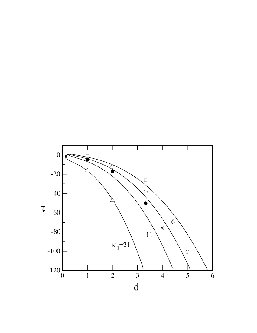
Figure 2: Values of $\tau$ as a function of inverse HS diameter ratio $d$, for various values of HSPC length–to–breadth ratio $\kappa_{1}$. Lines: Frozen–orientation approximation ($Q=0$); from top to bottom: $\kappa_{1}=6$, $8$, $11$ and $21$. Symbols: free orientations. Squares: $\kappa_{1}=5$; open circles: $\kappa_{1}=8$; filled circles: $\kappa_{1}=11$, and triangles: $\kappa_{1}=21$.

IV.2 Other hard rod–hard sphere mixtures: effect of particle shape

To investigate the effect of the shape of the rods on the depletion effect and, in turn, on the stability of the smectic phase, VeselyVeselyMP has recently considered parallel-rod models consisting of linear overlapping hard-sphere chains, hard ellipsoids and hard spheroellipsoids. Here we have studied, still in the approximation of frozen orientations, two additional types of hard particles: cylinders (HCYL) and parallelepipeds with a square transverse shape (HPAR). To minimize the effect of the different particle geometries, the particles were chosen to have the same volume (see later). In all cases the minority component continues to consist of hard spheres. The functions $f_{ij}(z)$, and also their Fourier transforms, can be calculated analytically in these cases. The relevant expressions can be found in the Appendix A.

Figure 3: (a) The $\tau$ parameter vs. $\kappa_{1}$ for different values of the parameter $d$ (indicated in the graph). (b) A zoom of (a) for small $\kappa_{1}$’s. (c) $\tau$ vs. $d$ for different values of $\kappa_{1}$ as indicated in the figure. (c) $\tau$ parameter as a function of $d$ for different values of $\kappa_{1}$, as indicated. Results for HSPC, HCYL, and HPAR are plotted with solid, dashed, and dotted lines, respectively.

Results for the $\tau$ parameter in the case of HCYL/HS and HPAR/HS mixtures, along with the previously considered HSPC/HS mixtures, are shown in Figs. 3(a)-(c). The $\tau$ parameter is plotted against the aspect ratio of the rods $\kappa_{1}$ in Fig. 3(a) for different values of the scaled inverse HS diameter $d=D_{1}/D_{2}$ ($D_{1}$ being the side length of the parallelepiped in the case of HPAR); Fig. 3(b) is a zoom of (a) in the region of small $\kappa_{1}$. Finally, the $\tau$ parameter against $d$ for different values $\kappa_{1}$ is plotted in Fig. 3(c). We can see from Fig. 3(a) that $\tau$ tends to decrease linearly, becoming negative for sufficiently large aspect ratios. This effect is more and more pronounced as the diameter of the HS is decreased. An interesting feature is that, when the diameter of HS is greater than that of the rod, depletion is larger, and therefore smectic stability is enhanced more substantially, as one goes from HPAR to HCYL or HSPC (note that these two are very similar). The opposite behaviour (i.e. depletion in HPAR is enhanced with respect to HCYL and HSPC) results when the HS diameter is equal or less than that of the HSPC [Fig. 3(a)]. For short rods $\tau$ exhibits oscillatory behaviour [see Fig. 3(b)]. Finally, fixing $\kappa_{1}$ and increasing $d$, we find that the $\tau$ parameter decreases as a cubic power-law in $d$ and that its value for HPAR is much less than that for HSPC or HCYL.

The linear and cubic dependences of $\tau$ with respect to $\kappa_{1}$ and $d$, respectively, can be elucidated from Eqn. (17) using the fact that the volume ratio can be expressed as $v_{1}/v_{2}=\kappa_{1}d^{3}$ for the HCYL case (the other cases being similar), while the squared ratio of Fourier transforms of the overlap functions tends asymptotically, for large $\kappa_{1}$ and $d$, to a constant. Simple calculations give, in this limit,

$$\tau_{\hbox{\tiny HC}}=\tau_{\hbox{\tiny HSPC}}=-\frac{3}{128}\left(\cos{\frac{k_{0}^{*}}{2}}\right)^{-2}\kappa_{1}d^{3}$$ (20)

with $k_{0}^{*}=k_{0}L_{1}$ the reduced wave number of the N–Sm spinodal instability in the one–component system.

To study the effect of a varying particle shape on the phase behaviour of the rod-sphere mixtures, we have performed a full minimization of the Helmholtz free-energy functional with respect to smectic-like density profiles of the rods [$\rho_{1}(z)$] and spheres [$\rho_{2}(z)$]. The minimization was carried out with respect to the Fourier amplitudes of the truncated Fourier expansion of the density profiles and smectic wave number (details are provided in Appendix B). The choice of a Fourier expansion is justified by the fact that the HS equilibrium density profiles obtained with this minimization differ very significantly from those obtained via the usual single–amplitude exponential parametrization, as shown in Fig. 4. We can see that the parametrization produces too sharp density peaks in the HS profile, which enhances the depletion effect.

Figure 4: Equilibrium density profiles of the equimolar HSPC–HS mixture (different components are labelled in the figure) resulting from minimization with respect to the Fourier amplitudes (solid lines) and with respect to a single–amplitude exponential parametrization (dashed lines). The HSPC has an aspect ratio $\kappa_{1}=10$ and its breadth coincides with the HS diameter, taken as unity. The pressure in reduced units was chosen to be $0.4$.

Since we would like to compare the results from the density–functional minimization of mixtures composed of rods of different geometries (HSPC, HCYL and HPAR), a sensible criterion is required to choose the sizes of the particles so as to make sure that these differences arise from the shape and not from different sizes and volumes. For this purpose we have used three different criteria: (i) all particles have the same diameter and the same length, (ii) all particles have the same length and the same volume, and (iii) all particles have the same aspect ratio and the same volume. Comparing the equilibrium density profiles resulting from use of these three criteria, we have concluded that differences between particles are minimised using the third criterion (these results are not shown here).

We have calculated, using the free, i.e. Fourier–based, minimization, the phase diagrams of binary mixtures of rods (HSPC, HCYL and HPAR) and HS. The HSPC and HS diameters were taken to be equal and adopted as unit of length. The aspect ratios of all the rods were set to 10, all particle volumes being the same. The following relations result:

$$D_{\hbox{\tiny HC}}=\left[1-\left(3\kappa_{\hbox{\tiny HSPC}}\right)^{-1}\right]^{-1/3}D_{\hbox{\tiny HSPC}},$$

$$D_{\hbox{\tiny HP}}=\left(\frac{\pi}{4}\right)^{1/3}D_{\hbox{\tiny HC}},\quad L_{\mu}=\kappa_{\hbox{\tiny HSPC}}D_{\mu},$$ (21)

with $\mu$=HSPC, HC or HP.

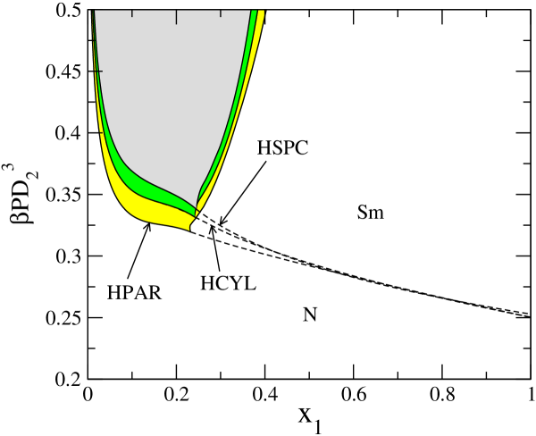
Figure 5: Phase diagrams in the reduced pressure–composition plane of three different mixtures composed of rods of different geometries (HSPC, HCYL, and HPAR) with HS. Different lines corresponding to each mixture are labelled in the figure. Also indicated are the stability regions of the nematic and the smectic phases. Solid lines represent the binodals of the N–Sm coexistence, while the continuous N–Sm transitions have been indicated by a dashed line.

The resulting phase diagrams are shown in Fig. 5. The first interesting feature of all phase diagrams is the presence of a tricritical point, where the nature of the N–Sm transition changes from second to first ordertricritical . For pressures higher than that of the tricritical point, the demixing instability region becomes wider. The width of this demixing window increases for mixtures going from HSPC to HCYL and then HPAR. This scenario clearly demonstrates that increasing differences in shape between spheres and rods enhance the depletion in smectics, resulting in a wider demixing gap.

IV.3 Zwanzig model: Onsager theory versus FMT

In order to check whether the effects presented above are robust with respect to the theory and approximations used, we have analysed a mixture of HPAR and HC using Fundamental–Measure theory in the Zwanzig approximation. Zwanzig Zwanzig introduced a model that considerably reduces the complexities associated with minimising a density-functional that depends on particle orientations. The approximation consists of restricting the possible orientations of a rod to lie along the three orthogonal axes $x,y$ and $z$, treating a pure system as a three-component mixture (one component for each orientation). The approximation is very useful and has been used quite substantially. In our FMT context, the resulting theory treats spatial correlations very accurately so that it should better describe the onset of smectic order in the nematic fluid. We have used the HPAR-HC system and the Zwanzig approximation because in this combination a FMT can be rigorously formulated Yuri . The Zwanzig approximation should not be terribly limiting, since the nematic fluid is well oriented. In order to elucidate the effect of restricted orientations separately from that inherent to the proper inclusion of higher–order correlations, a study of the HPAR-HC mixture using a Zwanzig–Onsager theory, together with that on mixtures of parallel HPAR and HC, is necessary.

IV.3.1 Zwanzig model in the Onsager formulation

In Appendix D we have written expressions for the Fourier transforms of the correlations functions $\tilde{c}_{ij}(k)$ as obtained from the Zwanzig–Onsager approach. These expressions are necessary to calculate the $\tau$ parameter using Eqn. (C.10). The results obtained are plotted in Fig. 6. In the same figure the parallel case is also plotted for the sake of comparison. The usual cubic power–law behaviour of $\tau$ with respect to $d$ is obtained; this is typical of any Onsager approach, as discussed in Sec. IV.2. The Zwanzig approach gives a lower value for $\tau$ as compared to the parallel case. This result is similar to that already obtained using the freely rotating Onsager approach for HSPC. For high values of $\kappa_{1}$, both approaches collapse into a single line, which is due to the high value of the order parameter $Q$ of a fluid composed of long particles.

Figure 6: $\tau$ parameter as a function of $d$ for three different values of $\kappa_{1}$, as indicated. Solid and dashed lines correspond to the Zwanzig and parallel approaches, respectively.

IV.3.2 Zwanzig model in the FMT formulation

Details on this approximation can be found in Ref. Yuri . Here we only give a brief sketch of the theory. We continue to use the notation introduced in the previous section for the dimensions of the particles, i.e. the length of the HPAR is $L_{1}$, the side length is $D_{1}$ (these particles are assumed to have a square section), and $D_{2}$ is the side length of the cubes. Since the unit vector $\hat{\bf\Omega}$ only has three possible orientations, the one–particle distribution functions $\rho_{s}({\bf r},\hat{\bf\Omega})$ can be expressed as

$$\rho_{s}({\bf r},\hat{\bf\Omega})=\sum_{\mu}\rho_{s\mu}({\bf r})\delta(\hat{\bf\Omega}-\hat{\bf e}_{\mu})$$ (22)

where $\hat{\bf e}_{\mu}$, $\mu=1,2,3$, are unit vectors along the three perpendicular directions $xyz$, respectively, and $\rho_{s\mu}({\bf r})$ are the local density of species $s$ parallel to the $\mu$-axis. The excess part of the free-energy density, in reduced thermal units, is obtained in Yuri , and has the form

$$\Phi_{\hbox{\tiny ex}}({\bf r};\{\rho_{s}\})=-n_{0}\ln(1-n_{3})+\frac{{\bf n}_{1}\cdot{\bf n}_{2}}{1-n_{3}}+\frac{n_{2x}n_{2y}n_{2z}}{(1-n_{3})^{2}},$$

(23)

with the functions $\{n_{\alpha}\}$ ($\alpha=\{0,1x,1y,1z,2x,2y,2z,3\}$) being weighted densities obtained as

$$n_{\alpha}({\bf r})=\sum_{s=1}^{2}\sum_{\mu=1}^{3}\int_{V}d{\bf r}^{\prime}\rho_{s\mu}({\bf r}^{\prime})\omega_{s\mu}^{(\alpha)}({\bf r}-{\bf r}^{\prime}),$$ (24)

where $\omega_{s\mu}^{(\alpha)}$ are characteristic functions whose spatial integrals give the fundamental measures of the particles (edge length, surface and volume). The ideal part of the free energy density in reduced thermal units for this model is

$$\Phi_{\rm{id}}(z)=\sum_{s\mu}\rho_{s\mu}(z)\left[\log\rho_{s\mu}(z)-1\right],$$ (25)

so that the total free energy per unit volume and unit thermal energy can be calculated as

$$\Phi=\frac{1}{d_{s}}\int_{0}^{d_{s}}dz\left[\Phi_{\rm{id}}(z)+\Phi_{\rm{exc}}(z)\right].$$ (26)

Density and order–parameter profiles can be defined; in particular, the density profile is

$$\rho_{s}(z)=\sum_{\mu}\rho_{s\mu}(z).$$ (27)

The nematic–smectic spinodal line can be obtained in this theory using the same kind of arguments used for the Onsager theory (Sec. II). Note, however, that the expression (17) for the $\tau$ parameter is not valid in this context, and we need to use the more general formula (C.10), valid for any mixture of freely rotating particles. In the Appendix C we describe in detail how this formula is obtained. An alternative way to calculate this parameter is to implement a numerical differentiation scheme on the spinodal line $\eta(\eta_{2})$.

The nematic–smectic spinodal lines for the case $\kappa_{1}=8$ and various values of the scaled cube side length $d^{-1}=D_{2}/D_{1}$ are shown in Fig. 7, whereas the corresponding $\tau$ parameters for different values of $\kappa_{1}$ are shown in Fig. 8. As was the case in the mixtures analysed using Onsager theory, $\tau$ decreases as the size of the cubes is diminished, indicating a stronger depletion effect and a corresponding enhancement of the smectic–phase stability.

Figure 7: Nematic–smectic spinodal line $\eta$–$\eta_{2}$, as obtained from Fundamental–Measure theory for the HPAR-HC mixture, for $\kappa_{1}=8$ and various values of $d^{-1}$, as indicated in the graph.

An interesting feature of these results is that they appear to exhibit linear behaviour for large values of $d$ (i.e. as the size of the cubes becomes smaller). Fig. 8 shows this by means of least–square fits to linear functions. The coefficients of the fit are functions of the aspect ratio $\kappa_{1}$, and, in turn, appear to be linear in $\kappa_{1}$, as shown in Fig. 9.

Figure 8: $\tau$ parameter as a function of $d$ for various values of the parallelepiped length–to–breadth $\kappa_{1}=L_{1}/D_{1}$ (indicated in the graph). The data are indicated by symbols; linear least-square fits $\tau=\alpha(\kappa_{1})+\beta(\kappa_{1})d$ are included as lines for each value of $\kappa_{1}$.

Figure 9: Symbols: coefficients $\alpha$ (circles) and $\beta$ (squares) as a function of $\kappa_{1}$. Solid lines: linear fits $\alpha(\kappa_{1})=\alpha_{1}+\alpha_{2}\kappa_{1}$ and $\beta(\kappa_{1})=\beta_{1}+\beta_{2}\kappa_{1}$, with $\beta_{2}=-0.038$.

To explain the linear behaviour obtained for the $\tau$ parameter as a function of $d$, we have analytically calculated the asymptotic behaviour of $\tau$ in the régime $d\gg 1$ for a mixture of parallel parallelepipeds and cubes in the FMT formulation. In Fig. 10 we compare the $\tau$ parameter, for various values of $\kappa_{1}$, obtained from the Zwanzig and parallel FMT approaches. An interesting feature is that depletion is enhanced in the Zwanzig approach, a result opposite to that from the Onsager approach (Fig. 6).

Figure 10: The $\tau$ parameter as a function of $d$ calculated from the Zwanzig (solid line) and parallel (dashed line) FMT approaches. Values of $\kappa_{1}$ are indicated as labels.

Details on the calculation of the asymptotic behaviour of $\tau$ with respect to $d$ have been relegated to Appendix F. From the general expression of $\tau$ (Eqn. C.10), particularized for the parallel case ($Q=1$, which makes the third terms in the numerator and denominator to vanish), the linear behaviour can be explained if the sum of the two terms in the numerator are of order $d^{-2}$. Since the volume ratio is $v_{1}/v_{2}=\kappa_{1}d^{3}$, we obtain the asymptotic behaviour $\tau\sim\kappa_{1}d=L_{1}/D_{2}$. This result can also be obtained using the Zwanzig model (Figs. 8 and 9), which shows that the third term of the numerator in Eqn. (C.10) is also of order $\sim d^{-2}$. The coefficient $\beta(\kappa_{1})$ of the linear fits of $\tau$ with respect to $\kappa_{1}$ (Fig. 9) depends linearly on $\kappa_{1}$ and has a slope $\beta_{2}=-0.038$ (see caption of Fig. 9), which is in the range of values predicted by the asymptotic limit of $W(\kappa_{1})\equiv\tau/(\kappa_{1}d)$ as a function of $\kappa_{1}$, shown in Fig. (11).

The function $\left(\partial\Delta/\partial\rho_{2}\right)^{(0)}$ [Eqn. (F.1)] is of order $d^{-2}$ only within the FMT formulation, the Onsager approach giving a term $\sim d^{0}$. This, in turn, shows the importance of properly taking account of pair correlations between particles in order to adequately describe depletion interactions. The asymptotic limit coincides with the adhesive limit because, when the mixture is highly asymmetric, the attractive depletion potential between two big particles becomes narrower and deeper, tending in the limit to a Dirac delta function at contact. This result is confirmed by our calculations in Appendix F, which show that the inverse Fourier transform of one of the terms of the function $\left(\partial\Delta/\partial\rho_{2}\right)^{(0)}$ is a Dirac delta function at contact. We have repeated the same analysis in Appendix F for the case of a HS binary mixture in the FMT formulation (PY approach). We have obtained that $\left(\partial\Delta/\partial\rho_{2}\right)^{(0)}_{\hbox{\tiny HS}}\sim{\cal O}(d^{-3})$. Also, a Dirac delta function at contact is present in the inverse Fourier transform of $\left(\partial\Delta/\partial\rho_{2}\right)^{(0)}$. The difference in the limit of infinite size asymmetry between the HPAR-HC and HS cases is due to the difference in particle shapes: when two big particles are closer enough the parallel sides of two parallelepipeds exclude many more small particles from their interstitial space than the curved surface of two big hard spheres. The discussion above forces us to speculate about the possible asymptotic behaviour of the $\tau$ parameter for the HSPC-HS mixture in the limit $d\gg 1$: since $v_{1}/v_{2}\sim d^{3}$, $\tau\sim{\cal O}(d^{0})$ [Eqns. (C.10) and (F.2)]; this is a consequence of the caps of the spherocylinders being spherical. This argument does not apply to the behaviour of $\tau$ in the limit of large $\kappa_{1}$ for fixed $d$, which continues to be linear.

V Conclusions and perspectives

The first result from this study on depletion effects in smectic phases is that, within Onsager theory, the inclusion of orientational degrees of freedom significantly reduces the enhanced stability of the smectic phase over the nematic phase as compared to that obtained from the frozen-orientation approximation. A second conclusion that can be drawn is that when the surface curvature of the rods is very different from that of the other species (e.g. the case of HPAR and HS), depletion is enhanced and the smectic phase stabilizes at lower packing fractions as HS become more abundant. This effect is also reflected in the fact that the N–Sm demixing gap in the phase diagram widens as one goes from HSPC to HP particles through the HC geometry. Finally, the inclusion of more realistic pair correlations between particles, in the manner of FMT theory, changes the asymptotic behaviour of the $\tau$ parameter (a convenient measure of depletion in smectics) for large values of the ratio $d$, i.e. the asymmetry between the breadth of the rod and the sphere diameter; in particular, for HPAR, $\tau$ increases linearly with $d$, while for HSPC we speculate that $\tau$ goes to a finite limit. The limiting case of large aspect ratios and finite $d$ is similarly captured by both Onsager and Fundamental–Measure theories.

In this work we have studied the depletion mechanism along the N–Sm spinodal line for different mixtures by explicit calculation of the $\tau$ parameter evaluated on this line in the pure fluid. An interesting task could be to extend this study to equilibrium smectic phases, consisting of well-developed density peaks, by defining some quantity evaluated at the smectic density profile. In this case depletion-based mechanisms may add interesting phenomenology, such as strong microsegregation between different species, which could be directly quantified using some suitably defined parameter. Work along this direction is currently in progress.

VI Appendix

Appendix A. Overlap functions: case of frozen orientations

When particle orientations are parallel, the functions $f_{ij}(z)$ and their Fourier transforms can be written exactly for a large class of particle shapes and their mixtures. We consider in turn each of the particle geometries analysed in the paper.

In the case of mixtures of HSPC of length $L_{1}$ and breadth $D_{1}$, and HS of diameter $D_{2}$, the Fourier transforms are

$$\tilde{f}_{11}(k) = \frac{4\pi}{k^{3}}\left\{\sin\left[k(D_{1}+L_{1})\right]\right.$$

$$- \left.D_{1}k\cos\left[k(D_{1}+L_{1})\right]-\sin\left(kL_{1}\right)\right\},$$

$$\tilde{f}_{12}(k) = \frac{4\pi}{k^{3}}\left\{\sin\left[(D_{12}+L_{1})k/2\right]\right.$$

$$- \left.\frac{k}{2}D_{12}\cos\left[(D_{12}+L_{1})k/2\right]-\sin\left(kL_{1}/2\right)\right\},$$

$$\tilde{f}_{22}(k) = \frac{4\pi}{k^{3}}\left[\sin\left(kD_{2}\right)-kD_{2}\cos\left(kD_{2}\right)\right],$$ (A.1)

where $D_{12}=D_{1}+D_{2}$.

For mixtures of HCYL of length $L_{1}$ and breadth $D_{1}$, and HS of diameter $D_{2}$, the appropriate Fourier transforms:

$$\tilde{f}_{11}(k) = \frac{2\pi D_{1}^{2}}{k}\sin\left(kL_{1}\right),$$

$$\tilde{f}_{12}(k) = 2\pi\Bigg{\{}\frac{D_{1}^{2}}{4k}\sin\left[\frac{k(L_{1}+D_{2})}{2}\right]-\frac{D_{2}}{k^{2}}\cos\left[\frac{k(L_{1}+D_{2})}{2}\right]$$

$$+ \frac{2}{k^{3}}\left[\sin\left[\frac{k(L_{1}+D_{2})}{2}\right]-\sin\left(\frac{kL_{1}}{2}\right)\right]$$

$$+ \frac{D_{1}D_{2}}{2k}\left[\frac{\pi}{2}\left[\cos\left(\frac{kL_{1}}{2}\right)J_{1}\left(\frac{kD_{2}}{2}\right)\right.\right.$$

$$- \left.\left.\sin\left(\frac{kL_{1}}{2}\right)H_{1}\left(\frac{kD_{2}}{2}\right)\right]+\sin\left(\frac{kL_{1}}{2}\right)\right]\Bigg{\}},$$

$$\tilde{f}_{22}(k) = \frac{4\pi}{k^{3}}\left[\sin\left(kD_{2}\right)-kD_{2}\cos\left(kD_{2}\right)\right]$$ (A.2)

where $J_{1}(x)$ and $H_{1}(x)$ are the Bessel and Struve functions of first order, respectively.

For mixtures of HPAR with length and square side length $L_{1}$, $D_{1}$, respectively, and HS of diameter $D_{2}$, the Fourier transforms are

$$\tilde{f}_{11}(k) = \frac{8D_{1}^{2}}{k}\sin\left(kL_{1}\right),$$

$$\tilde{f}_{12}(k) = 8\left\{\left(\frac{D_{1}}{2}\right)^{2}\frac{\sin{[k(L_{1}+D_{2})/2]}}{k}\right.$$

$$+ \left.\frac{\pi}{4}\left[\frac{2}{k^{3}}\left(\sin{\left[\frac{k(L_{1}+D_{2})}{2}\right]}-\sin{\frac{kL_{1}}{2}}\right)\right.\right.$$

$$- \left.\left.\frac{D_{2}}{k^{2}}\cos{\left[\frac{k(L_{1}+D_{2})}{2}\right]}\right]\right.$$

$$\left.+\right. \left.\frac{D_{1}D_{2}}{2k}\left[\frac{\pi}{2}\left[\cos{\left(\frac{kL_{1}}{2}\right)}J_{1}\left(\frac{kD_{2}}{2}\right)\right.\right.\right.$$

$$- \left.\left.\left.\sin{\left(\frac{kL_{1}}{2}\right)}H_{1}\left(\frac{kD_{2}}{2}\right)\right]+\sin{\left(\frac{kL_{1}}{2}\right)}\right]\right\},$$

$$\tilde{f}_{22}(k) = \frac{4\pi}{k^{3}}\left[\sin\left(kD_{2}\right)-kD_{2}\cos\left(kD_{2}\right)\right].$$ (A.3)

Appendix B. Minimisation of Onsager functional in the frozen-orientation approximation

We assume a Fourier expansion for the density profiles $\rho_{i}(z)$:

$$\rho_{i}(z)\equiv\rho x_{i}\psi_{i}(z)=\rho x_{i}\left(1+\sum_{n=1}^{\infty}s_{n}^{(i)}\cos{nkz}\right),$$ (B.1)

with $k$ the smectic wave number, and $s_{n}^{(i)}$ the $n$-th Fourier amplitude for species $i$. Introducing this expression into the free-energy funtional, Eqn. (1), we obtain

$$\Phi=\rho\Bigg{\{}\log\rho-1 + \sum_{i}x_{i}\ln x_{i}+\frac{x_{i}}{d_{s}}\int_{0}^{d_{s}}dz\psi_{i}\left(z\right)\ln\psi_{i}\left(z\right)$$ (B.2)

$$+ \rho{\cal W}(x,k,\{s_{k}^{(i)}\})\Bigg{\}},$$

Here we have expressed the excess part in terms of the function

$${\cal W}(x,k,\{s_{n}^{(i)}\})=\frac{1}{2}\sum_{i,j}x_{i}x_{j}$$

$$\hskip 28.45274pt\times\left[\tilde{f}_{ij}(0)+\frac{1}{2}\sum_{n=1}^{\infty}s_{n}^{(i)}s_{n}^{(j)}\tilde{f}_{ij}(k_{n})\right],$$ (B.3)

where $k_{n}=nk$ and the Fourier transforms $\tilde{f}_{ij}(k)$ were defined in Section II (since we are assuming perfect orientational order, we set $Q=1$). From this, the pressure is

$$\beta P=\rho+\rho^{2}{\cal W}(x,k,\{s_{n}^{(i)}\})$$ (B.4)

To calculate phase equilibria in the mixture it is more convenient to work in conditions of constant pressure. Then, we minimize the Gibbs free energy per particle and unit thermal energy,

$$g\equiv\frac{1}{\rho}\left(\Phi+\beta P\right)$$ (B.5)

with respect to the smectic wave number and the coefficients $\{s_{n}^{(i)}\}$. The corresponding derivatives can be written down explicitely but they have to be solved numerically using an iterative method. In practice, the Fourier expansions have been truncated; they include ca. 40 terms so as to satisfy a stringent convergence criterion in the iterative procedure (the number of Fourier amplitudes was chosen to guarantee an absolute error less than $10^{-7}$ in the density profiles).

Appendix C. $\tau$ parameter: general case

The strategy is to obtain the nematic–smectic spinodal line perturbatively in the composition $x$, since we only need to know the spinodal in the neighbourhood of $x=0$ to obtain the $\tau$ parameter. The equations to solve are three: two defining the spinodal, the third giving the equilibrium state of the nematic fluid on the spinodal [Eqns. (9)]. These equations can be written as

$$\Delta(k,\rho_{1},\rho_{2},Q)=\left[1-\rho_{1}\tilde{c}_{11}(k,\rho_{1},\rho_{2},Q)\right]$$

$$\times\left[1-\rho_{2}\tilde{c}_{22}(k,\rho_{1},\rho_{2},Q)\right]-\rho_{1}\rho_{2}\tilde{c}_{12}^{2}(k,\rho_{1},\rho_{2},Q)=0$$

(C.1)

$$\frac{\partial\Delta(k,\rho_{1},\rho_{2},Q)}{\partial k}=0$$ (C.2)

$$\frac{\partial\Phi(\rho_{1},\rho_{2},Q)}{\partial Q}=0,$$ (C.3)

where $\tilde{c}_{ij}(k,\rho_{1},\rho_{2},Q)$ are the Fourier transforms of the direct correlation functions between species $i$ and $j$. The relationship between infinitesimal changes in the variables $\{k,\rho_{1},\rho_{2},Q\}$ along the spinodal can be calculated from (C.1) as

$$\left(\frac{\partial\Delta}{\partial\rho_{1}}\right)d\rho_{1}+\left(\frac{\partial\Delta}{\partial\rho_{2}}\right)d\rho_{2}+\left(\frac{\partial\Delta}{\partial Q}\right)dQ+\left(\frac{\partial\Delta}{\partial k}\right)dk=0.$$

(C.4)

Similarly, the relation between the changes in the order parameter $Q$ and densities $\{\rho_{1},\rho_{2}\}$ can be obtained from (C.3) as

$$\left(\frac{\partial^{2}\Phi}{\partial Q\partial\rho_{1}}\right)d\rho_{1}+\left(\frac{\partial^{2}\Phi}{\partial Q\partial\rho_{2}}\right)d\rho_{2}+\left(\frac{\partial^{2}\Phi}{\partial Q^{2}}\right)dQ=0.$$

(C.5)

Defining the coefficient $\upsilon\equiv d\rho_{1}/d\rho_{2}$, we obtain from Eqns. (C.4) and (C.5):

$$\upsilon=-\frac{\displaystyle{\left(\frac{\partial\Delta}{\partial\rho_{2}}\right)-\left(\frac{\partial\Delta}{\partial Q}\right)\frac{\left(\partial^{2}\Phi/\partial Q\partial\rho_{2}\right)}{\left(\partial^{2}\Phi/\partial Q^{2}\right)}}}{\displaystyle{\left(\frac{\partial\Delta}{\partial\rho_{1}}\right)-\left(\frac{\partial\Delta}{\partial Q}\right)\frac{\left(\partial^{2}\Phi/\partial Q\partial\rho_{1}\right)}{\left(\partial^{2}\Phi/\partial Q^{2}\right)}}},$$ (C.6)

where the condition given in (C.2) of the absolute minimum of $\Delta(k,\rho_{1},\rho_{2},Q)$ with respect to the wave number $k$ was used. Note that this expression is valid for any composition $x$ of the mixture. Now, evaluating all the derivatives at $\rho_{2}=0$ we obtain, from Eqn. (C.1)

$$\left(\frac{\partial\Delta}{\partial\rho_{1}}\right)^{(0)} = -\rho_{0}\left[\left(\frac{\partial\tilde{c}_{11}}{\partial\rho_{1}}\right)^{(0)}+\frac{\tilde{c}_{11}^{(0)}}{\rho_{0}}\right],$$ (C.7)

$$\left(\frac{\partial\Delta}{\partial\rho_{2}}\right)^{(0)} = -\rho_{0}\left[\left(\frac{\partial\tilde{c}_{11}}{\partial\rho_{2}}\right)^{(0)}+\left(\tilde{c}_{12}^{(0)}\right)^{2}\right],$$ (C.8)

$$\left(\frac{\partial\Delta}{\partial Q}\right)^{(0)} = -\rho_{0}\left(\frac{\partial\tilde{c}_{11}}{\partial Q}\right)^{(0)},$$ (C.9)

where the superscripts mean that all derivatives are evaluated at $x=0$, $k=k_{0}$, and $Q=Q_{0}$, values corresponding to the one-component fluid spinodal [note that, from Eqn. (C.1), we get $1-\rho_{0}\tilde{c}_{11}=0$ at $\rho_{2}=0$, which has been used to obtain the derivatives above].

Now, using the fact that, for the one-component fluid, $1-\rho_{0}\tilde{c}^{(0)}_{11}=0$, and that the $\tau$ parameter can be expressed through the coefficient $\upsilon$ evaluated at $x=0$ as $\tau=1+(v_{1}/v_{2})\upsilon^{(0)}$, we finally obtain

$$\tau=1-\frac{v_{1}}{v_{2}}$$

$$\times\frac{\displaystyle{\left(\tilde{c}_{12}^{(0)}\right)^{2}+\left(\frac{\partial\tilde{c}_{11}}{\partial\rho_{2}}\right)^{(0)}-\left(\frac{\partial\tilde{c}_{11}}{\partial Q}\right)^{(0)}\frac{\left(\partial^{2}\Phi/\partial\rho_{2}\partial Q\right)^{(0)}}{\left(\partial^{2}\Phi/\partial Q^{2}\right)^{(0)}}}}{\displaystyle{\left(\tilde{c}_{11}^{(0)}\right)^{2}+\left(\frac{\partial\tilde{c}_{11}}{\partial\rho_{1}}\right)^{(0)}-\left(\frac{\partial\tilde{c}_{11}}{\partial Q}\right)^{(0)}\frac{\left(\partial^{2}\Phi/\partial\rho_{1}\partial Q\right)^{(0)}}{\left(\partial^{2}\Phi/\partial Q^{2}\right)^{(0)}}}}$$

(C.10)

which is a general expression for the $\tau$ parameter. In the Onsager approximation, we have $\tilde{c}_{ij}(k,\rho_{1},\rho_{2},Q)=\tilde{f}_{ij}(k,Q)$ and the derivatives of $\tilde{c}_{ij}$ with respect to the densities $\rho_{i}$ vanish, while for parallel rods ($Q=1$) the derivative with respect to $Q$ also vanishes, and we obtain expression (17).

For a fluid mixture of particles without orientational degrees of freedom, such as a mixture of parallel parallelepipeds and cubes or a mixture of hard spheres, expression (C.10) for $\tau$ can be reinterpreted as follows. From Eqn. (C.10), the $\tau$ parameter can be re-expressed as

$$\tau=1-\frac{v_{1}}{v_{2}}\frac{\displaystyle{\left(\frac{\partial S_{ef}^{-1}}{\partial\rho_{2}}\right)^{(0)}}}{\displaystyle{\left(\frac{\partial S_{ef}^{-1}}{\partial\rho_{1}}\right)^{(0)}}},$$ (C.11)

where $S^{-1}_{ef}(k,\rho_{1},\rho_{2})$ is the inverse structure factor of an effective one-component fluid of particles, labelled as 1, with interactions between them being mediated by particles labelled as 2. This structure factor can be calculated by evaluating the second functional derivative with respect to $\rho_{1}({\bf r})$ of the semi-grand canonical free-energy functional

$$\Upsilon[\rho_{1}]\equiv F[\rho_{1},\rho_{2}]-\mu_{2}\int d{\bf r}\rho_{2}({\bf r}),$$ (C.12)

at the bulk densitiesCuesta . Here $F[\rho_{1},\rho_{2}]$ is the Helmholtz free-energy functional of the binary mixture and the density profile $\rho_{2}({\bf r})$ in Eqn. (C.12) is calculated from the condition of fixed chemical potential of species 2:

$$\frac{\delta F[\rho_{1},\rho_{2}]}{\delta\rho_{2}({\bf r})}=\mu_{2}.$$ (C.13)

The result for this effective structure factor is

$$S_{eff}^{-1}(k,\rho_{1},\rho_{2}) = 1-\rho_{1}\tilde{c}_{11}(k,\rho_{1},\rho_{2})$$ (C.14)

$$- \frac{\rho_{1}\rho_{2}\tilde{c}^{2}_{12}(k,\rho_{1},\rho_{2})}{1-\rho_{2}\tilde{c}_{22}(k,\rho_{1},\rho_{2})}.$$

After the inclusion of its first derivative with respect to $\rho_{1}$ and $\rho_{2}$, evaluated at $\rho_{2}=0$ in Eqn. (C.11), we exactly obtain Eqn. (C.10) without the third terms in both numerator and denominator (as they vanish for fluids without orientational degrees of freedom).

Appendix D. Correlation functions for HPAR-HC mixture in the Zwanzig–Onsager approach

In the Zwanzig approximation the rods point along one of the Cartesian axes $x,y$ or $z$. For the binary HP-HC mixture in the Zwanzig approach the correlation functions evaluated at ${\bf k}=(0,0,k)$ can be calculated as

$$-\tilde{c}_{11}(k) = 2x_{\perp}^{2}\left[\tilde{f}_{1x,1x}(k)+\tilde{f}_{1x,1y}(k)\right]+x_{\parallel}^{2}\tilde{f}_{1z,1z}(k)$$ (D.1)

$$+ 4x_{\perp}x_{\parallel}\tilde{f}_{1x,1z}(k),$$

$$-\tilde{c}_{12}(k) = 2x_{\perp}\tilde{f}_{1x,2}(k)+x_{\parallel}\tilde{f}_{1z,2}(k),$$ (D.2)

$$-\tilde{c}_{22}(k) = \tilde{f}_{22}(k),$$ (D.3)

where the subindexes $1\mu$ ($\mu=x,y,z$) label particle 1 (rods), which point along the direction $\mu$, while the subindex 2 labels cubes. $x_{\perp}$ and $x_{\parallel}$ are respectively the fraction of rods perpendicular and parallel to the nematic director (which is taken to be parallel to the $z$ axis). These variables are functions of the nematic order parameter $Q$ [i.e. $x_{\perp}=(1-Q)/3$, and $x_{\parallel}=(1+2Q)/3$], the equilibrium values of which should be calculated from the extremum condition of the free-energy density with respect to $Q$. This condition reads

$$\frac{\partial\Phi}{\partial Q}=\frac{2}{3}\rho_{1}\left\{\ln\left[\frac{1+2Q}{1-Q}\right]-2\rho_{1}\left(L_{1}-D_{1}\right)^{2}D_{1}Q\right\}=0$$

The expressions for the Fourier-transformed overlap functions are

$$\tilde{f}_{1x,1y}(k)=2(L_{1}+D_{1})^{2}\frac{\sin(kD_{1})}{k},$$

$$\tilde{f}_{1x,1x}(k)=8L_{1}D_{1}\frac{\sin(kD_{1})}{k},$$

$$\tilde{f}_{1x,1z}(k)=4D_{1}(L_{1}+D_{1})\frac{\sin\left[k(L_{1}+D_{1})/2\right]}{k},$$

$$\tilde{f}_{1z,1z}(k)=8D_{1}^{2}\frac{\sin(kL_{1})}{k},$$

$$\tilde{f}_{1x,2}(k)=2(L_{1}+D_{2})(D_{1}+D_{2})\frac{\sin\left[k(D_{1}+D_{2})/2\right]}{k},$$

$$\tilde{f}_{22}(k)=8D_{2}^{2}\frac{\sin(kD_{2})}{k},$$

$$\tilde{f}_{1z,2}(k)=2(D_{1}+D_{2})^{2}\frac{\sin\left[k(L_{1}+D_{2})/2\right]}{k},$$ (D.5)

Note that, due to the discrete axial symmetry of the particles, some overlap functions can be expressed in terms of others; for instance, $\tilde{f}_{1x,1x}=\tilde{f}_{1y,1y}$, and $\tilde{f}_{1z,1x}=\tilde{f}_{1z,1y}$.

Appendix E. Correlation functions for HPAR-HC and HS mixtures in the FMT approach

To obtain the Fourier transforms of the correlation functions for HP-HC mixtures Yuri , and for HS mixtures Rosenfeld , we have used the FMT functional, which has the same structure in both systems, namely:

$$-\tilde{c}_{ij}({\bf k}) = \chi^{(0)}\tilde{f}_{ij}({\bf k})+\boldsymbol{\chi}^{(1)}\tilde{\boldsymbol{R}}_{ij}({\bf k})+\boldsymbol{\chi}^{(2)}\tilde{\boldsymbol{S}}_{ij}({\bf k})$$ (E.1)

$$+ \chi^{(3)}\tilde{V}_{ij}({\bf k}),$$

where $\tilde{f}_{ij}$, $\tilde{\boldsymbol{R}}_{ij}$, $\tilde{\boldsymbol{S}}_{ij}$ and $\tilde{V}_{ij}$ are Fourier transforms of the overlap function, and of the mean radius, surface and volume of the overlap region between particles $i$ and $j$, respectively. For a HPAR-HC mixture the mean radius and the surface area of the overlap region are vectors oriented along the directions parallel to the edge lengths (mean radius) and perpendicular to the sides (surface area) of the parallelepipeds. For the HS mixture they are scalars, as are the quantities $\chi^{(1)}$ and $\chi^{(2)}$, which for the HPAR-HC mixture are vectors. Finally, the correlation functions depend on the wave vector ${\bf k}$ or on its module $k$ in the HPAR-HC and HS mixtures, respectively. The expressions for $\chi^{(i)}$ corresponding to the HPAR-HC mixture are

$$\chi^{(0)} = \frac{1}{1-\eta},\quad\boldsymbol{\chi}^{(1)}=\frac{\boldsymbol{\xi_{2}}}{(1-\eta)^{2}},$$ (E.2)

$$\boldsymbol{\chi}^{(2)} = \frac{\boldsymbol{\xi_{1}}}{(1-\eta)^{2}}+\frac{2\boldsymbol{\zeta}_{2}}{(1-\eta)^{3}},$$ (E.3)

$$\chi^{(3)} = \frac{\rho}{(1-\eta)^{2}}+\frac{2\boldsymbol{\xi}_{1}\boldsymbol{\xi}_{2}}{(1-\eta)^{3}}+\frac{6\xi_{2x}\xi_{2y}\xi_{2z}}{(1-\eta)^{4}}$$ (E.4)

with $\rho=\sum_{i}\rho_{i}$ and $\eta=\sum_{i}\rho_{i}v_{i}$ the total density and packing fraction, respectively, $\boldsymbol{\zeta}_{2}=(\xi_{2y}\xi_{2z},\xi_{2z}\xi_{2x},\xi_{2x}\xi_{2y})$, and

$$\xi_{1x}=\xi_{1y}=\sum_{i}\rho_{i}D_{i},\quad\xi_{1z}=\rho_{1}L_{1}+\rho_{2}D_{2},$$ (E.5)

$$\xi_{2x}=\xi_{2y}=\rho_{1}L_{1}D_{1}+\rho_{2}D_{2}^{2},\quad\xi_{2z}=\sum_{i}\rho_{i}D_{i}^{2},$$ (E.6)

with $L_{1}$ and $D_{1}$ the length and breadth of the parallelepiped, while $D_{2}$ is the edge-length of the cube.For the HS mixture we have

$$\chi^{(0)} = \frac{1}{1-\eta},\quad\chi^{(1)}=\frac{\xi_{2}}{(1-\eta)^{2}},$$ (E.7)

$$\chi^{(2)} = \frac{\xi_{1}}{(1-\eta)^{2}}+\frac{1}{4\pi}\frac{\xi_{2}^{2}}{(1-\eta)^{3}},$$ (E.8)

$$\chi^{(3)} = \frac{\rho}{(1-\eta)^{2}}+\frac{2\xi_{1}\xi_{2}}{(1-\eta)^{3}}+\frac{1}{4\pi}\frac{\xi_{2}^{3}}{(1-\eta)^{4}},$$ (E.9)

where

$$\xi_{1}=\frac{1}{2}\sum_{i}\rho_{i}D_{i},\quad\xi_{2}=\pi\sum_{i}\rho_{i}D_{i}^{2},$$ (E.10)

and $D_{i}$ ($i=1,2$) the particle diameters.

To calculate the $\tau$ parameter we only need expressions for $\tilde{c}_{11}$ and $\tilde{c}_{12}$. The Fourier transforms of the geometric measures of overlapping bodies for the HPAR-HC fluid with a wave number ${\bf k}=(0,0,k)$ (smectic symmetry) are

$$\tilde{f}_{11}(k) = 8D_{1}^{2}\frac{\sin(kL_{1})}{k},$$ (E.11)

$$\tilde{\boldsymbol{R}}_{11}(k) = 4D_{1}^{2}\left[D_{1}\frac{\sin(kL_{1})}{k},D_{1}\frac{\sin(kL_{1})}{k},\right.$$ (E.12)

$$\left.4\left(\frac{\sin(kL_{1}/2)}{k}\right)^{2}\right],$$

$$\tilde{\boldsymbol{S}}_{11}(k) = 2D_{1}^{3}\left[4\left(\frac{\sin(kL_{1}/2)}{k}\right)^{2},4\left(\frac{\sin(kL_{1}/2)}{k}\right)^{2},\right.$$ (E.13)

$$\left.D_{1}\frac{\sin(kL_{1})}{k}\right],$$

$$\tilde{V}_{11}(q) = 4D_{1}^{4}\left(\frac{\sin(kL_{1}/2)}{k}\right)^{2}$$ (E.14)

The expressions for particles 1 and 2 are

$$\tilde{f}_{12}(k) = 2D_{12}^{2}\frac{\sin(kL_{12}/2)}{k}$$ (E.15)

$$\tilde{\boldsymbol{R}}_{12}(k) = 2D_{12}\left[D_{1}D_{2}\frac{\sin(kL_{12}/2)}{k},D_{1}D_{2}\frac{\sin(kL_{12}/2)}{k},\right.$$ (E.16)

$$\left.2D_{12}\frac{\sin(kL_{1}/2)\sin(kD_{2}/2)}{k^{2}}\right],$$

$$\tilde{\boldsymbol{S}}_{12}(q) = 2D_{1}D_{2}\left[2D_{12}\frac{\sin(kL_{1}/2)\sin(kD_{2}/2)}{k^{2}},\right.$$

$$\left.2D_{12}\frac{\sin(kL_{1}/2)\sin(kD_{2}/2)}{k^{2}},\right.$$

$$\left.D_{1}D_{2}\frac{\sin(kL_{12}/2)}{k}\right]$$

$$\tilde{V}_{12}(q) = 4(D_{1}D_{2})^{2}\frac{\sin(kL_{1}/2)\sin(kD_{2}/2)}{k^{2}},$$ (E.18)

where $D_{12}=D_{1}+D_{2}$ and $L_{12}=L_{1}+D_{2}$.

For HS mixtures these expressions have the form

$$\tilde{f}_{ij}(k) = \frac{4\pi}{k^{2}}\left[\frac{\sin(kD_{ij}/2)}{k}-\frac{D_{ij}}{2}\cos(kD_{ij}/2)\right],$$ (E.19)

$$\tilde{R}_{ij}(k) = \frac{4\pi}{k^{2}}\left[\frac{\sin(kD_{i}/2)\sin(kD_{j}/2)}{k^{2}}\right.$$ (E.20)

$$- \left.\frac{D_{i}D_{j}}{4}\cos(kD_{ij}/2)\right],$$

$$\tilde{S}_{ij}(k) = \frac{(4\pi)^{2}}{k^{2}}\left[\frac{D_{ij}}{2}\frac{\sin(kD_{i}/2)\sin(kD_{j}/2)}{k^{2}}\right.$$ (E.21)

$$- \left.\frac{D_{i}D_{j}}{4}\frac{\sin(kD_{ij}/2)}{k}\right],$$

$$\tilde{V}_{ij}(k) = \frac{(4\pi)^{2}}{k^{4}}\left[\frac{\sin(kD_{i}/2)\sin(kD_{j}/2)}{k^{2}}-\frac{\sin(kD_{ij}/2)}{k}\right.$$ (E.22)

$$+ \left.\cos(kD_{i}/2)\cos(kD_{j}/2)\right],$$

for $i,j=1,2$.

Appendix F. Asymptotic behaviour of $\tau$

The asymptotic behaviour of $\left(\partial\Delta/\partial\rho_{2}\right)^{(0)}$ for $d=D_{1}/D_{2}\gg 1$ can be calculated from (C.8) and (E.1), particularizing the latter equation to HPAR-HC and HS mixtures. After some algebra, we arrive at

$$\left(\frac{\partial\Delta}{\partial\rho_{2}}\right)^{(0)}_{HPAR}=-\rho_{0}\left[\left(\tilde{c}_{12}^{(0)}\right)^{2}+\left(\frac{\partial\tilde{c}_{11}}{\partial\rho_{2}}\right)^{(0)}\right]$$

$$\sim - \frac{v_{1}}{d^{2}}y(1+y)\left\{2(1+y)^{2}T_{1}^{2}(k_{0}^{*}/2)\right.$$ (F.1)

$$+ \left.\left[T_{0}(k^{*}_{0})+2yT_{1}(k_{0}^{*})+y^{2}T_{1}^{2}(k^{*}_{0}/2)\right]\kappa_{1}^{-2}\right\},$$

where $\kappa_{1}=L_{1}/D_{1}$, $T_{0}(x)=\cos{x}$, and $T_{1}(x)=\sin{x}/x$, while $y=\eta_{0}/(1-\eta_{0})$, and $k^{*}_{0}=k_{0}L_{1}$. The expression corresponding to the HS fluid reads

$$\left(\frac{\partial\Delta}{\partial\rho_{2}}\right)^{(0)}_{HS} \sim -\frac{v_{1}}{d^{3}}y(1+y)\left\{2y^{2}(1+3y)T_{V}(k^{*}_{0})+T_{\delta}(k_{0}^{*})\right.$$ (F.2)

$$+ \left.2yT_{f}(k_{0}^{*})+y(1+6y)T_{S}(k_{0}^{*})\right\},$$

where we have defined the dimensionless quantities $T_{V}(k_{0}^{*})=6v_{1}^{-2}\tilde{V}(k^{*}_{0})$, $T_{\delta}(k_{0}^{*})=3s_{1}^{-1}\tilde{\delta}(k_{0}^{*})$, $T_{f}(k_{0}^{*})=3v_{1}^{-1}\tilde{f}(k_{0}^{*})$, and $T_{S}(k_{0}^{*})=6(v_{1}s_{1})^{-1}\tilde{S}(k_{0}^{*})$, with $s_{1}$ and $v_{1}$ the surface area and volume of particle 1, while $\tilde{\delta}(q)$ is the Fourier transform of the Dirac delta function $\delta(D_{1}-|{\bf r}|)$. The presence of a delta function indicates that, in the limit $d\to\infty$, the one-component sticky-sphere limit of the fluid is obtained. We arrive at the same conclusion, in the same limit, for the HPAR/HC mixture, by comparing Eqns. (F.1) and (F.2). Each term in the right-hand side of Eqn. (F.1), from left to right, has the same meaning as in the HS mixture: they are related to the Fourier transform of the volume, adhesiveness, overlap function, and surface area of the overlap region between two particles, respectively. For example, the inverse Fourier transform of $T_{0}(k^{*})$, with the smectic symmetry ${\bf q}=(0,0,q)$, results in a term proportional to $\delta(L_{1}-|z|)/2$, which reflects the stickiness of parallelepipeds along the $z$ direction. A complete effective density functional for the infinite asymmetric limit was worked out for hard-cube mixtures in Ref.YuriCuesta . The direct correlation function resulting from this functional has a Dirac delta function located at contact of the sides of the cubes.

However, there is an important difference between the HP-HC and HS mixtures, which is related to the square and cubic power dependence of the expressions (F.1) and (F.2) with respect to the asymmetric parameter $d=D_{1}/D_{2}$. This result is related to the fact that the planar geometry of the sides of parallelepipeds enhances the depletion interaction between two big particles. We should compare these results with those obtained using the Onsager approach, where $\tilde{c}_{ij}(k,\rho_{1},\rho_{2})=\tilde{f}_{ij}(k)$ and then $\left(\partial\Delta/\partial\rho_{2}\right)^{(0)}\sim{\cal O}(d^{0})$. Thus, we can conclude that depletion interactions in this limit cannot be properly described by the Onsager approximation.

Finally, to obtain the asymptotic behaviour of the $\tau$ parameter for the HP-HC mixture in the limit $d\to\infty$ , we use Eqns. (C.10), (F.1) and (E.1), particularized for HP, together with the spinodal instability condition $1-\rho_{0}\tilde{c}_{11}^{(0)}=0$, to obtain explicitly

$$\tau\sim\kappa_{1}dW(\kappa_{1}),$$ (F.3)

$$W(\kappa_{1})=-\left\{2(1+y)^{2}T_{1}^{2}(k_{0}^{*}/2)+\left[T_{0}(k^{*}_{0})+2yT_{1}(k_{0}^{*})\right.\right.$$

$$+\left.\left.y^{2}T_{1}^{2}(k^{*}_{0}/2)\right]\kappa_{1}^{-2}\right\}\left\{y^{-1}\left(3+y^{-1}\right)+2(3+y)T_{1}(k_{0}^{*})\right.$$

$$-\left.\left[3+y+6(1+y)^{3}\right]T_{1}^{2}(k_{0}^{*})\right\}^{-1}$$ (F.4)

In Fig. (11) the function $W(\kappa_{1})$ is plotted. As can be seen from the figure, (i) $W$ varies very little with respect to $\kappa_{1}$, and (ii) depletion is maximum in the Onsager limit ($\kappa_{1}\to\infty$). Note that, on taking the latter limit, the condition $d=D_{1}/D_{2}\gg 1$ must be fulfilled.

It is well known that, when the PY approximation is used, the condition $1-\rho_{0}\tilde{c}_{11}(k,\rho_{0})>0$ is always fulfilled for all $\eta$ and $q$ in the physical parameter region. Because of the absence of a fluid-solid spinodal in this approximation, we cannot calculate the $\tau$ parameter to estimate the effect of depletion at the freezing transition.

Figure 11: The function $W(\kappa_{1})$.

References

- (1) M. Adams, S. Fraden, Biophys. J. 74, (1998) 669.
- (2) M. Adams, Z. Dogic, S.L. Keller, S. Fraden, Nature 393, (1998) 349.
- (3) Z. Dogic, S. Fraden, Current Opinion in Colloid & Interface Science 11, (2006) 47.
- (4) D. L. Cheung and M. P. Allen, Phys. Rev. E 74, (2006) 021701.
- (5) D. Andrienko, M. Tasinkevych, P. Patricio, M. P.Allen, and M. M. Telo da Gamma, Phys. Rev. E 68, (2003) 051702.
- (6) R. Roth, R.van Roij, D. Andrienko, K. R. Mecke, and S. Dietrich, Phys. Rev. Lett. 89, (2002) 088301.
- (7) T. Koda, M. Numajiri, S. Ikeda, J. Phys. Soc. Jap. 65, (1996) 3551.
- (8) T. Koda, S. Ikeda, Mol. Cryst. Liq. Cryst. 318, (1998) 101.
- (9) T. Koda, Y. Sato, S. Ikeda, Prog. Theor. Phys. Suppl. 138, (2000) 476.
- (10) Z. Dogic, D. Frenkel, and S. Fraden, Phys. Rev. E 62, (2000) 3925.
- (11) G. Cinacchi, E. Velasco, L. Mederos, J. Phys. Cond. Matter 16, (2004) S2003;
- (12) S. Lago, A. Cuetos, B. Martínez–Haya, L. F. Rull, J. Molecular Recognition 17, (2004) 417.
- (13) F. J. Vesely, Mol. Phys. 103, (2005) 679.
- (14) L. Onsager, Ann. N.Y. Acad. Sci. 51, (1949) 627.
- (15) G. Cinacchi, L. Mederos, E. Velasco, J. Chem. Phys. 121, (2004) 3854.
- (16) Y. Rosenfeld, J. Chem. Phys. 89, 4272 (1988); Phys. Rev. Lett. 63, (1989) 980.
- (17) J. A. Cuesta and Y. Martínez–Ratón, Phys. Rev. Lett. 78, (1997) 3691; J. Chem. Phys. 107, (1997) 6379.
- (18) A. Esztermann, H. Reich, M. Schmidt, Phys. Rev. E 73, (2006) 011409.
- (19) S. Asakura and F. Oosawa, J. Chem. Phys. 22, 1255 (1954); J. Polym. Sci. 33, 183 (1958).
- (20) Tricritical points are predicted by a large number of models for liquid crystals and other systems, even in pure fluids. In particular, the present phase diagram is topologically equivalent to that predicted by the Blume-Emery-Griffiths model [Phys. Rev. A 4, 1071 (1971)] for a He4–He3 mixture, identifying rods with He4, spheres with He3 and inverse temperature with reduced pressure.
- (21) R. Zwanzig, J. Chem. Phys. 39, 1714 (1963).
- (22) J. A. Cuesta and Y. Martínez-Ratón, J. Phys: Condens. Matter 11, (1999) 10107.
- (23) Y. Martínez-Ratón and J. A. Cuesta, Phys. Rev. E 58, (1998) R4080.