Sensitivity of solar off-limb line profiles to electron density stratification and the velocity distribution anisotropy

The effect of the electron density stratification on the intensity profiles of the H i Ly-$\alpha$ line and the O vi and Mg x doublets formed in solar coronal holes is investigated. We employ an analytical 2-D model of the large scale coronal magnetic field that provides a good representation of the corona at the minimum of solar activity. We use the mass-flux conservation equation to determine the outflow speed of the solar wind at any location in the solar corona and take into account the integration along the line of sight (LOS). The main assumption we make is that no anisotropy in the kinetic temperature of the coronal species is considered. We find that at distances greater than 1 $R_{\sun}$ from the solar surface the widths of the emitted lines of O vi and Mg x are sensitive to the details of the adopted electron density stratification. However, Ly-$\alpha$, which is a pure radiative line, is hardly affected. The calculated total intensities of Ly-$\alpha$ and the O vi doublet depend to a lesser degree on the density stratification and are comparable to the observed ones for most of the considered density models. The widths of the observed profiles of Ly-$\alpha$ and Mg x are well reproduced by most of the considered electron density stratifications, while for the O vi doublet only few stratifications give satisfying results. The densities deduced from SOHO data result in O vi profiles whose widths and intensity ratio are relatively close to the values observed by UVCS although only isotropic velocity distributions are employed. These density profiles also reproduce the other considered observables with good accuracy. Thus the need for a strong anisotropy of the velocity distribution (i.e. a temperature anisotropy) is not so clear cut as previous investigations of UVCS data suggested. However, these results do not rule completely out the existence of some degree of anisotropy in the corona. The results of the present computations also suggest that the data can also be reproduced if protons, heavy ions and electrons have a common temperature, if the hydrogen and heavy-ion spectral lines are also non-thermally broadened by a roughly equal amount.

1 Introduction

Extreme-ultraviolet (EUV) spectral lines provide valuable information on the plasma conditions in the solar wind acceleration zone. Information on the densities, the temperatures, the bulk velocities and the velocity distributions of different species, can be obtained from the total intensity, Doppler width and shift of multiple line profiles with the appropriate instrument. Basically three techniques are used to deduce both bulk velocity and the velocity distribution.

The first is the usual Doppler effect that provides information on the LOS velocity of the emitting source. The second is the Doppler dimming which yields information on (microscopic and macroscopic) velocity components not directed along the LOS, on the basis of the technique proposed by Rompolt (1967 & 1969) and Hyder & Lites (1970). See, e.g., Beckers & Chipman (1974) for a description. Note that Doppler dimming acts only on the radiative component of a line. Rompolt (1967, 1969 & 1980), Heinzel & Rompolt (1987) and Gontikakis et al. (1997a,b) used the Doppler dimming of Ly-$\alpha$ to study moving prominences. It has later been considered to diagnose the solar wind (Kohl & Withbroe 1982; Withbroe et al. 1982; Strachan et al. 1989 & 1993; etc.).

Optical pumping is a third process. It happens when, due to the Doppler effect, the absorption profile of the moving atom overlaps with a neighboring incident spectral line. This is the case for the coronal O vi 1037.61 Å line that can be excited by the chromospheric C ii doublet at 1036.3367 and 1037.0182 Å when the solar wind speed reaches values between $\sim 100$ and $\sim 500$ km s^-1 (Noci et al. 1987; Kohl et al. 1998; Li et al. 1998). Finally, Cranmer et al. (1999a) used optical pumping by Fe iii 1035.77 Å to diagnose wind speeds around $\sim 530$ km s^-1.

UVCS (the UltraViolet Coronagraph Spectrometer; Kohl et al. 1995 & 1997) on the SOHO (the SOlar and Heliospheric Observatory; Domingo et al. 1995) mission yielded valuable data on the solar corona, including the polar coronal holes up to more than 3.5 $R_{\sun}$ (Kohl et al. 1997 & 1998; Noci et al. 1997; Habbal et al. 1997; Li et al. 1998; etc.). One of the most exciting results obtained from data recorded by UVCS concerns the very broad lines emitted by heavy ions (namely O vi and Mg x) in polar coronal holes during the minimum of the solar activity cycle. From the analysis of profiles of coronal lines (mainly the Ly-$\alpha$, O vi and Mg x doublets) Kohl et al. (1997 & 1998), Noci et al. (1997) and others concluded that the evidence for highly anisotropic velocity distributions of the cited species is strong. For O vi and Mg x the ratio of kinetic temperatures in the directions perpendicular and parallel to the coronal magnetic field, respectively, is found to range from 10 to more than 100 (Kohl et al. 1997 & 1998; Cranmer et al. 1999b; etc.). In addition, the heavy ions are deduced to be significantly hotter and faster than the protons (Li et al. 1997).

In the present paper we extend the work of Raouafi & Solanki (2004; hereafter abbreviated as RS04) in different ways. Firstly, we consider a more complete set of published density profiles. Secondly, we study the effect of the density stratification on spectral lines having very different formation mechanisms: Ly-$\alpha$ is purely radiative; Mg x lines are exclusively collisional and the O vi doublet results from both mechanisms. In addition, we also calculate the LOS integrated total intensities of the Ly-$\alpha$ and O vi lines.

2 Line formation in the corona

In an optically thin medium, the general form of the contribution to the emissivity of a given point on the LOS, assuming a Maxwellian velocity distribution and a Gaussian shaped incident profile, is given by

$$\begin{array}[]{l}{\displaystyle{\cal{I}}(\nu)=\int_{LOS}{\rm{d}}Z\;\Bigg{\{}\frac{N_{X^{n+}}(\theta)\,{N_{\rm e}}(\theta)\,{\alpha}_{lu}}{4\,\pi\,\sqrt{\pi}\,\alpha_{s}}\,{\rm{e}}^{-\left(\frac{\delta\nu-\frac{\nu_{0}}{c}u_{Z}}{\alpha_{s}}\right)^{2}}}\\ \;\;\;+{\displaystyle\frac{N_{X^{n+}}(\theta)\,B_{lu}\,{\cal{I}}_{R}}{\left(4\,\pi\right)^{2}}}{\displaystyle\int_{\Omega}\!{\rm{d}}\Omega\;\left[f\times{\cal{D}}\times{\cal{P}}\times{\cal{M}}\right](\Omega,\theta)\Bigg{\}}};\end{array}$$ (3)

where $N_{X^{n+}}(\theta)$ and ${N_{\rm{e}}}(\theta)$ are densities of scattering ions $X^{n+}$ and electrons (cm^-3), respectively. $B_{lu}$ and ${\alpha}_{lu}$ are the Einstein coefficient for absorption between the two atomic levels $l$ and $u$ and the coefficient of electronic collisions, respectively. The width of the microscopic velocity distribution $\alpha_{s}$ is assumed to be isotropic (no anisotropy in the kinetic temperature of scattering atoms/ions is considered throughout this paper)). $\alpha_{s}$ includes the contribution due to thermal motions. ${\displaystyle\delta\nu=\nu-\nu_{0}}$, where $\nu_{0}$ is the rest frequency of the reemitted line. The geometry of the scattering process is given by Fig. 1 in RS04. The other terms entering Eq. (3) are defined in the same paper. The different values of the coefficient ${\cal{W}}_{ul}$ in the expression of ${\cal{M}}(\Omega,\theta)$ and the corresponding spectral lines studied here are given in Table 1. Eq. (3) is general and applies to any spectral line irrespective of whether it is formed by collisions and/or by radiation. An exception is when the incident profiles deviates from a Gaussian (see Sect. 5.1 on how such a case can be dealt with).

Table 1: Values of ${\cal{W}}_{ul}$ for the spectral lines considered here.

$J_{l}$	$J_{u}$	${\cal{W}}_{ul}$	Examples of spectral lines
$\displaystyle\frac{1}{2}$	$\displaystyle\frac{1}{2}$	0	Mg x 624.941 Å, O vi 1037.61 Å
			H i 1215.6736 Å
$\displaystyle\frac{1}{2}$	$\displaystyle\frac{3}{2}$	0.5	Mg x 609.793 Å, O vi 1031.92 Å
			H i 1215.6682 Å

Figure 1: Electron density plotted as a function of the distance to Sun center for different empirical models (solid curve: DKL (Doyle et al. 1999a,b; Kohl et al. 1998; and Lamy et al. 1997) dotted: Guhathakurta et al. 1999; Dashes: Guhathakurta & Holzer 1994; Dot-dashes: Cranmer et al. 1999c; Triple-dot-dashes: Esser et al. 1999).

According to Eq. (3), the profiles created by collisions and by resonant scattering at a given point along the LOS all have Gaussian shapes. However, there are significant differences between the two components. The main differences are:
1) The intensity of the collisional component is proportional to the square of the electron density, where as the radiative component is only proportional to the density. Thus, the collisional component suffers the radial density drop more than the radiative one.
2) The radiative component is affected by the outflow speed of the scattering ions through the Doppler dimming effect, while the collisional component is not. Thus, the contributions to the collisional component from sections along the LOS supporting large outflow speeds are more important than the contributions to the radiative one, since the latter gets progressively out of resonance due to the increase in outflow speed of the solar wind with the distance from Sun center.
3) For a given point on the LOS, the Doppler shift of the collisional component reflects the real LOS speed $u_{Z}$ of the scattering atoms/ions. The shift of the radiative component, however, corresponds to only a fraction of this speed. This point is very important for the broadening of the line profile. Note that in frame of the complete redistribution approximation, there is no shift difference between collisionally and radiatively excited profiles (see Sahal-Bréchot & Raouafi 2005).

3 Atmospheric parameters

The realistic synthesis of spectral line profiles requires the modeling of all the parameters entering the formation process of a given spectral line. According to Eq. (3), this includes the magnetic field, the solar wind outflow velocity, the density stratifications of electrons and of atoms/ions, etc., at every point along the LOS. For the large scale magnetic field of the corona and the solar wind velocity we adopt the same descriptions as RS04, while for the density stratifications we consider a wider range of models.

The coronal magnetic field is described by the model of Banaszkiewicz et al. (1998; see Fig. 1 of RS04). Cranmer et al. (1999c) used the same model to constrain the strength and superradial expansion of the magnetic field in the corona. The solar wind outflow speed is obtained through the mass-flux conservation equation

$$\begin{array}[]{c}{\displaystyle V(r,\theta)=\frac{Ne(R_{\sun})}{Ne(r,\theta)}\,\frac{B(r,\theta)}{B(R_{\sun},\theta_{\sun})}\,V(R_{\sun},\theta_{\sun})},\end{array}$$ (5)

where $Ne(R_{\sun}),\,V(R_{\sun},\theta_{\sun})$ and $B(R_{\sun},\theta_{\sun})$ are the electron density, the outflow speed of the ions and the coronal magnetic field at the base of the solar corona (solar surface), respectively. $Ne(r,\theta),\;V(r,\theta)$ and $B(r,\theta)$ are the same quantities at coordinates $(r,\theta)$, with $r>R_{\sun}$. The angles $\theta$ and $\theta_{\sun}$ are related to each other by the requirement that Eq. (5) is valid along a field line. This also implies that the velocity vector is parallel to the magnetic field vector (needed for the calculation of the dimming rate of the radiative component and also for the determination of the Doppler shift of the reemitted spectral line). In order to be consistent with Ulysses observations that the fast solar wind varies by less than a few percent with latitude (Neugebauer et al. 1998; McComas et al. 2000; Zhang et al. 2002), we adopt $V(R_{\sun},\theta_{\sun})\propto B(R_{\sun},\theta_{\sun})$ as boundary condition on the outflow speed on the solar surface (see Table 2). We consider different values of $V_{\sun}$ for the different species. We also consider different $V_{\sun}$ for the different density stratification models in order to get as close as possible to the observed values of widths, total intensities and intensity ratios.

Table 2: Proportionality coefficient, $\kappa$, of $V(R_{\sun},\theta_{\sun})$ to $B(R_{\sun},\theta_{\sun})$ $\left(\displaystyle{{V(R_{\sun},\theta_{\sun})}=\kappa\times{B(R_{\sun},\theta_{\sun})}}\right)$ used for the calculations of the different spectral lines considered in the present paper and corresponding to the different density models.

	DKL	Guhathakurta & Holzer	Guhathakurta et al.	Cranmer et al.	Esser et al.
		(1994)	(1999)	(1999c)	(1999)
H i	0.63	0.85	0.35	0.30	0.13
O vi	0.85	0.88	0.50	0.35	0.13
Mg x	0.85	0.88	0.50	0.35	0.13

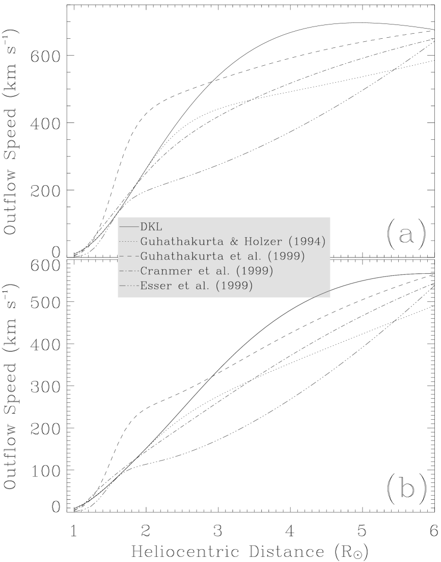
Figure 2: Outflow speed of the O vi ions along the polar axis and field line arising from 70 degree latitude, respectively, for the different density models considered. The Boundary condition on the outflow speed of the coronal ions is chosen to be proportional to the solar surface magnetic field strength (see text). In order to get as close as possible to the measured values, we adopt different values of the proportionality coefficient of $V(R_{\sun},\theta_{\sun})$ with respect to $B(R_{\sun},\theta_{\sun})$ for the different density models. The outflow speed of other species can be obtained by multiplying the present ones by a constant.

RS04 have shown that the density stratification is a key quantity for determining the off-limb profiles of collision-dominated lines, in particular the line width. Here we consider a more complete set of empirical density stratifications than in that paper. In addition to the electron density profiles from (Doyle et al. 1999a,b; hereafter abbreviated as DKL) determined empirically by combining the results obtained by three instruments on SOHO (SUMER: Doyle et al. 1999a,b; UVCS: Kohl et al. 1999; LASCO: Lamy et al. 1997) and from Guhathakurta & Holzer (1994; SKYLAB) which were considered by RS04, we also employ the models of Guhathakurta et al. (1999; SPARTAN), Cranmer et al. (1999c) and Esser et al. (1999; SPARTAN and Mauna Loa; Fisher & Guhathakurta 1995). The absolute values of the density in all these models are not very different. They are generally within the error bars of the coronal densities which are typically 20 - 30 % of the measured values (the main exception is the Esser et al. model). Except for the DKL model, the data for the other models has been fitted by power series functions based on the fact that the density drops very fast close to the Sun and follows an $\sim{r^{-2}}$ function sufficiently far away. The description given by Doyle et al. for the DKL electron density stratification (Eq. (13) of RS04) assumes that the coronal gas is isothermal and in hydrostatic equilibrium (see Guhathakurta & Fisher 1995 & 1998).

The absolute value of the electron density directly affects the intensity of the emitted line at any point along the LOS. However, the importance of the density stratification resides therein that it also influences the LOS-integrated profile indirectly through the solar wind speed, which is determined via mass-flux conservation and thus depends on both the density stratification and the magnetic field. Even somewhat different density stratifications give quite different solar wind speeds and therefore very different line profiles. A more thorough discussion is given in the following Sects. The effect of the density stratification on the outflow speed and LOS velocity has been illustrated by RS04; see their Fig. 5.

The solar wind speed profiles obtained for the combination of the chosen magnetic structure and the density stratifications are plotted in Fig. 2 for two extreme cases. In Fig. 2(a) the wind speed along the polar axis is displayed, while Fig. 2(b) shows the speed along the field line arising from 70 degree latitude on the solar surface. The LOS at $3.5\leavevmode\nobreak\ R_{\sun}$ intersects this field line at $6\leavevmode\nobreak\ R_{\sun}$, which is the distance to which we integrate the profiles.

The small decrease in the solar wind speed at high altitudes (solid line in panel a) indicates some mismatch between the DKL model and the Banaszkiewicz et al. magnetic structure right above the pole. This decrease does not affect our conclusions since it occurs at altitudes above $4\leavevmode\nobreak\ R_{\sun}$, whereas the furthest LOS we consider passes at $3.5\leavevmode\nobreak\ R_{\sun}$ above the pole.

The scaling factors of the solar wind speed at the solar surface are listed in Table 2. Clearly although the scaling factors of the heavy elements are not the same as for hydrogen, they differ by less than a factor of 1.5, with the hydrogen atoms moving more slowly.

In order to compute the total intensities of the lines emitted in the polar coronal holes, we need the absolute density of each ion $N_{X^{n+}}$, a parameter not considered by RS04. It can be written as follows

$$\begin{array}[]{l}{\displaystyle N_{X^{n+}}=\frac{N_{X^{n+}}}{N_{X}}\,\frac{N_{X}}{N_{H}}\,\frac{N_{H}}{N_{\rm{e}}}\,N_{\rm{e}}},\end{array}$$ (7)

where ${\displaystyle({N_{X^{n+}}}/{N_{X}}})$ is obtained from the ionization balance of the $X$ species, ${\displaystyle({N_{X}}/{N_{H}}})$ is the abundance of X relative to hydrogen and ${\displaystyle({N_{H}}/{N_{\rm{e}}}})$ is the abundance of Hydrogen relative to electrons. Here we adopt a plasma with 10% of helium (the cosmic value) so that ${\displaystyle{N_{H}}/{N_{\rm{e}}}=0.83}$. However, the coronal helium abundance could be considerably larger and could vary significantly through the region considered here (see Joselyn & Holzer 1978; Hansteen, Holzer & Leer 1993, Hansteen, Leer & Holzer 1994a,b & 1997). The considered fraction of neutral hydrogen is $2.667\leavevmode\nobreak\ 10^{-7}$ (John Raymond, private communication). ${\displaystyle{N_{O^{5+}}}/{N_{O}}}=4.78\leavevmode\nobreak\ 10^{-3}$ (Nahar 1999) and the abundance of oxygen relative to hydrogen is taken to be 8.7 (Asplund et al. 2004).

4 Effect of the integration along the LOS on the collisional and radiative components

The results that will be presented in the present Sect. are obtained by using the DKL density stratification. The use of any of the other density models does not change the conclusions.

UVCS samples three types of lines: the Mg x lines at 609.793 Å and 624.941 Å are only excited by electron collisions, while the Ly-$\alpha$ line is exclusively created by resonant scattering of the solar disk radiation. The contribution of the collisional component is negligible (less than 1% according to Raymond et al. 1997). The O vi lines at 1031.92 Å and 1037.61 Å are excited by the combination of collisions and scattering of the transition region radiation.

Here we consider separately the collisional and radiative components of the considered coronal spectral lines in order to illustrate better the effects of the solar wind outflow velocity, density stratification and the integration along the LOS on each of them. The behavior of a particular line depends on the relative strengths of these two components.

Figs. 3 and 4 display the profiles emitted from different sections along the LOS for two different projected heliocentric distances 1.5 and $3.5\leavevmode\nobreak\ R_{\sun}$ (i.e. different rays) for spectral lines created solely by electron collisions and purely from resonant scattering of the solar disk radiation, respectively. For the sake of clarity, we used constant $\alpha_{s}$ to illustrate the effect of the LOS integration on the profiles in Figs. 3, 4 & 5. When comparing with observed profiles in Sect. 5, however, we only consider computations with height-dependent $\alpha_{s}$.

At low altitudes ($<2\leavevmode\nobreak\ R_{\sun}$) the main contribution is given by the central part of the LOS (i.e. near the polar axis). This is due to the fast drop of the densities as a function of the heliocentric distance (Fig.1). However, when further from the solar disk, significant contributions are obtained from larger sections (larger $|Z|$) along the LOS, due to the relatively slow decrease of the densities far from the solar limb ( Fig. 1). Doppler dimming, which is largest at greater heights, concentrates the contribution of the radiative component to the observed line profile toward small $|Z|$ (compare the bottom panels of Figs. 3 & 4). Another striking difference is seen in the Doppler shift behavior of the two components. The Doppler shift of the collisional profiles increases when moving away from the polar axis along the LOS (Fig. 3). The Doppler sift of the radiative component also increases at small $|Z|$, but ever more slowly at larger $|Z|$. Depending on the profile of the LOS velocity, the line shift can reach a limiting value characteristic of that LOS, or can even start to decrease again at greater $|Z|$ (Fig. 4).

Figure 3: Contributions to the final line profile emanating from different sections of the LOS (different values of $Z$) for a spectral line excited only by electron collisions (namely a Mg x doublet line) for LOSs coming to within $0.5\leavevmode\nobreak\ R_{\sun}$ and $2.5\leavevmode\nobreak\ R_{\sun}$ of the solar surface (top and bottom frames, respectively). The LOS integrated profile is the sum of all the individual profiles emitted by the different sections along the LOS. The marked $Z$ values are in units of $R_{\sun}$. Blue Doppler shifts correspond to positive LOS speeds (toward the observer) that are obtained for positive values of $Z$.

Figure 4: Equivalent results as in Fig.3 but for a purely radiatively excited line.

The behavior seen in Figs. 3 & 4 can be understood as follows. At a given $Z$, the Doppler shift of the collisional component is equal to the LOS speed $u_{Z}$ of the scattering atoms/ions (see first term of the RHS of Eq. (3)). However, for the radiative component the Doppler shift is given by ${\displaystyle(u_{Z}-\alpha_{si}\,n_{Z}\,\textbf{{u}}\cdot\textbf{{n}})}$. For small $|Z|$ (close to the pole where the field lines are only slightly inclined with respect to the polar axis), $n_{Z}$ is very small and the Doppler shift is approximately equal to $u_{Z}$, so that collisional and radiative line profiles arising at small $|Z|$ are similar. However, further away from the polar axis, $n_{Z}$ increases (in absolute value) so that, depending on $n_{Z}$ and $\alpha_{si}$ $(=\alpha_{s}^{2}/(\alpha_{i}^{2}+\alpha_{s}^{2}))$, the expression ${\displaystyle(u_{Z}-\alpha_{si}\,n_{Z}\,\textbf{{u}}\cdot\textbf{{n}})}$ either saturates or even decreases again ($\alpha_{i}$ is the Doppler width of the incident line profile). This effect is more marked at higher altitudes where the contribution from LOS sections with large $|Z|$ are important (see bottom panel of Fig. 4).

Figure 5: Line profiles obtained by integrating over different distances between $-Z_{0}$ and $Z_{0}$ along the LOS for a spectral line excited only by electron collisions (a) and only by radiation (b). These profiles are obtained for a point of closest approach of $3.5\leavevmode\nobreak\ R_{\sun}$ from Sun center and for $\alpha_{s}=200$ km s^-1 ($\alpha_{i}=100$ km s^-1 for the radiative component). The effect of the LOS integration on the radiatively excited line is rather small compared to the collisional line.

In Fig. 5 profiles for a purely collisionally (a) and purely radiatively (b) excited line are displayed. The plotted lines are obtained by integrating out to different distances along the LOS for a projected heliocentric distance of $3.5\leavevmode\nobreak\ R_{\sun}$. Profiles of collisional lines turn out to be sensitive to the atmospheric parameters, in particular LOS velocity, out to $|Z|=6\leavevmode\nobreak\ R_{\sun}$. The profile shape of the radiatively excited line is hardly altered by LOS integration, although the total intensity is significantly affected (not visible in Fig. 5 due to the normalization).

5 Application to coronal lines

Among the spectral lines observed by UVCS in polar coronal holes three sets are of particular interest. The first is the most intense line emitted in the solar corona, Ly-$\alpha$. This line is produced by the resonant scattering of the radiation emitted by the solar disk. The few electron collisions are negligible for this line (Raymond et al. 1997). The second group of lines is the O vi doublet. These lines are excited by both, the radiation coming from the underlying chromosphere-corona transition zone and by isotropic electron collisions. The third class is composed of the Mg x doublet, whose members are emitted following excitations produced almost exclusively by electron collisions (Wilhelm et al. 2004).

The dependence of $\alpha_{s}$ on $r$ and $\theta$ is computed consistently. We assume that $\alpha_{s}$ depends only on $r$, so that its value changes along the LOS. In the next subsections, we describe calculations of the profiles of these three sets of lines and their comparison with the observed ones.

5.1 The Ly-$\alpha$ line of hydrogen

Figure 6: Disk emission (+ signs) of Ly-$\alpha$ during the minimum of solar activity (Lemaire et al. 1998). The solid curve is a four-Gaussian fit to the data. The individual Gaussians contributing to the fit are given by the dotted, dashed, dot-dashed and triple-dot-dashed lines.

To calculate the coronal emission H Ly-$\alpha$, it is necessary to know the shape of the line profile coming from the solar disk (Fig. 6). A four Gaussian fit plus a constant background is applied to the complex shape of the observed profile. Numerically, we assume that coronal hydrogen atoms are illuminated by the photons of four incident Gaussian profiles emitted by the solar disk, with of course different parameters, as listed in Table 3. We do not consider any center-to-limb variation in the intensity emitted by the solar disk in Ly-$\alpha$ ($f(\Omega,\theta)=1$), which is in accordance with the filter images of Bonnet et al. (1980).

Figure 7: Widths (a) and total intensities (b) of the LOS-integrated Ly-$\alpha$ line profile as a function of the projected heliocentric distance obtained for the different density stratification models presented in Fig. 1. The correspondence symbols to density models are given in the top panel. The solid lines is the best fits to the observations recorded by UVCS and the dot-dashed line (top panel) is the turbulence velocity distribution of the hydrogen atoms. The vertical lines are the statistic error bars of the measurements.

Table 3: Parameters of the different Gaussians used to fit the Ly-$\alpha$ line. The Gaussians’ centers are given in (km s^-1) with respect to the line center as obtained from the data (+ signs in Fig. 6). The amplitudes are in ($10^{12}$ photons/cm²/s/(km s^-1) and the widths are in (km s^-1).

Gaussian	Amplitude	Position	Width
Dotted	0.22	-94.01	16.81
Dashed	2.24	-54.79	34.39
Dot-dashed	2.70	7.41	125.28
Triple-dot-dashed	2.13	65.13	34.91

A single Gaussian is sufficient to fit the calculated off-limb Ly-$\alpha$ profiles with good accuracy. Fig. 7(a) displays the e-folding (Doppler) widths of the LOS integrated Ly-$\alpha$ profiles as a function of the projected heliocentric distance on the plane of the sky (the widths of the best-fit Gaussian are plotted). The values of $\alpha_{s}$ used to reproduce these profiles are also given in the same Figure (dot-dashed line) together with the best fit to the observational data (solid line) by Cranmer et al. (1999a) (see also Kohl et al. 1998).

The computed Ly-$\alpha$ profiles are relatively in-sensitive to the details of the electron density stratification. For most of the density stratifications given in Fig. 1, the observed line width of Ly-$\alpha$ in polar coronal holes at different heights above the solar limb are comparable to the calculated ones in the presence of an isotropic velocity distribution and a gradual rise in $\alpha_{s}$ with projected distance to the limb. The displayed results are all located in the 1-$\sigma$ error bars of measured widths except for the widths obtained at low altitudes by using densities given by Guhathakurta et al. (1999) or between 2.3 and $2.7\leavevmode\nobreak\ R_{\sun}$ based on the Esser et al. densities. The reasons for these departures are visible in Fig. 2; note the high/low outflow speeds obtained through these density models at these altitudes. Note that the outflow speed of the hydrogen atoms at the solar surface is a free parameter. By lowering the outflow speed at $1\leavevmode\nobreak\ R_{\sun}$ (solar surface) for Guhathakurta et al. (1999) we can obtain a better correspondence with the measured widths a low altitudes. However, this occurs only at the cost of lower widths also at higher altitudes, so that the overall correspondence with the data is not improved.

Fig. 7(a) shows how the contribution to the line width from the small-scale velocity distribution, given by $\alpha_{s}$, which dominates at small $r$ is replaced by contributions from the outflowing solar wind at larger $r$, as the line width significantly exceeds the $\alpha_{s}$ value.

Fig. 7(a) also demonstrates that a more rapid drop in density with height leads to broader line profiles (compare profiles resulting from the DKL stratification with that of Guhathakurta et al. 1999). This means that of the two oppositely directed effects introduced by a steeper density gradient, a more rapidly increasing wind speed and a smaller contribution to the measured line profile from large $|Z|$ values, the former dominates.

Fig. 7(b) displays the total intensity of Ly-$\alpha$ as a function of the projected heliocentric distance for the different density stratifications considered in the present paper. The best fit to the observed intensities (solid curve) and the error bars of the measurements (vertical bars) are also plotted (see Cranmer et al. 1999a). All the density models considered give total intensities that are close to the observed ones (within a factor of $2-3$).

5.2 O vi doublet

We compute the intensity profiles of the lines of the O vi doublet at 1031.92 Å $\left(2s\;^{2}{\rm{S}}_{1/2}-2p\;^{2}{\rm{P}}_{3/2}\right)$ and 1037.61 Å $\left(2s\;^{2}{\rm{S}}_{1/2}-2p\;^{2}{\rm{P}}_{1/2}\right)$. In the solar corona, the O vi ions interact with electrons (with isotropic velocity distribution) and with the radiation coming from the underlying transition region. The effects of the ions’ motion are taken into account via the Doppler dimming, the Doppler shift and the optical pumping of the O vi 1037.61 Å line by the chromospheric C ii doublet (1036.3367 Å & 1037.0182 Å). This last effect is important above $\sim 2\leavevmode\nobreak\ R_{\sun}$ where the solar wind outflow speed reaches values that enable optical pumping to occur (the exact radius at which this occurs depends on the adopted solar wind profile). The incident solar disk spectrum considered for the calculations of the coronal O vi lines is shown in Fig. 2 of RS04. All the line profiles are assumed to be Gaussians. In the present computations, the radiances of the individual members of the O vi doublet on the disk spectrum are equated to 305 and 152.5 erg cm^-2 s^-1 sr^-1, respectively. Both O vi incident lines are assumed to have the same widths, corresponding to 35 km s^-1. We consider also two identical profiles for the C ii doublet with widths of 25 km s^-1 and radiances of 52 erg cm^-2 s^-1 sr^-1 each. We use the limb-brightening measured by Raouafi et al. (2002) for the O vi line and no limb-brightening for the C ii lines (see Warren et al. 1998). For comparison, Table 1 of RS04 presents different values of these parameters measured from different observations.

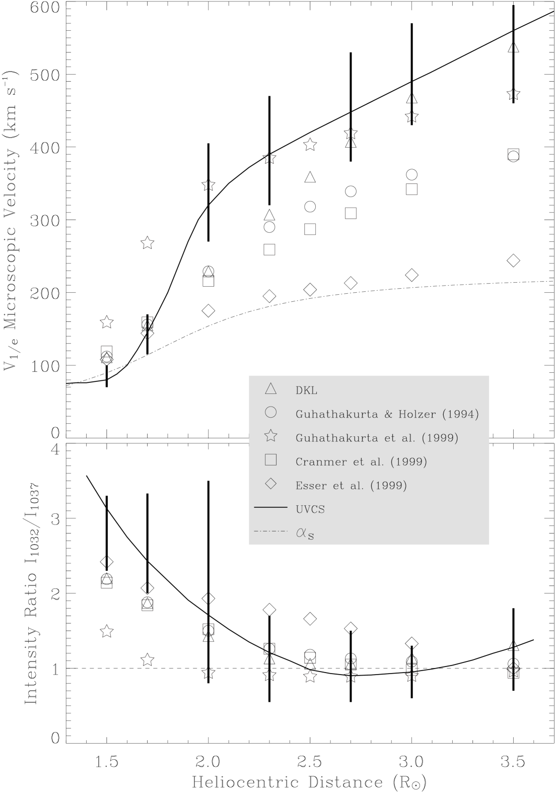
Figure 8: The symbols represent the variation of the width (top panel) and intensity ratio (bottom panel) of the LOS integrated synthetic line profiles of O vi as a function of the heliocentric distance. The correspondence between symbols and models is indicated in the grey frame. The dot-dashed curve displays the used values of $\alpha_{s}$. The observed dependence is given by the solid curves (best fits to the observations; see Cranmer et al. 1999c), with the vertical lines being error bars.

Figure 9: Total intensities of the O vi lines as a function of the projected heliocentric distance. The correspondence to the different density stratifications is given by the symbols in the top panel. The solid curves are the best fits to the observed intensities by UVCS and the vertical bars represent estimates of the accuracy of the observations.

Figure 10: LOS integrated profiles of the O vi 1031.92 Å line obtained at a projected heliocentric distance of $3.5\leavevmode\nobreak\ R_{\sun}$ for the different electron density stratifications considered in the present paper. The obtained line profiles are all approximatively Gaussian shaped, although they differ strongly in width.

The top panel of Fig. 8 displays the widths of the O vi 1031.92 Å line calculated for rays (LOSs) corresponding to different projected heliocentric distances and for different density stratification models. These widths are obtained by applying a Gaussian fit to each calculated profile. All profiles are well represented by a Gaussian. The profiles at the furthest considered ray ($3.5\leavevmode\nobreak\ R_{\sun}$) show the strongest departure from a Gaussian shape. They are plotted for all considered density models in Fig. 10. The solid line represents the best fit to the UVCS data (Cranmer et al. 1999a). Note that no anisotropy in the kinetic temperature of the emitting ions is considered.

At small heights ($<2\leavevmode\nobreak\ R_{\sun}$) the widths of the calculated profile are comparable for most of the density models except for the one by Guhathakurta et al. (1999). For this model the boundary condition on the solar wind speed at the solar surface is chosen to fit the widths at high latitudes. This gives higher solar wind speeds already at $1.5\leavevmode\nobreak\ R_{\sun}$ and explains the broader profiles resulting from this model at low altitudes. At larger heights $(>2.0\leavevmode\nobreak\ R_{\sun})$ the line widths are very sensitive to the details of the electron density stratification. This can be easily seen by the difference in the width of the different profiles obtained through slightly different density stratification models. The model by DKL gives line widths comparable to the ones obtained from the data, except between 2 and $2.7\leavevmode\nobreak\ R_{\sun}$, where the obtained widths are slightly smaller than the observed ones.

The bottom panel of Fig. 8 displays the ratio of total intensities of the O vi doublet lines $({\cal{I}}_{1032}/{\cal{I}}_{1037})$ as a function a the projected heliocentric distance. This ratio exhibits a marked dependence on radial distance being well over 2 close to the Sun, then dropping rapidly (except for the density models by Esser et al. 1999, which produces larger ratios compared to the ones given by the other density models and which do not fit the observations in particular at distances between 2.3 and $3\leavevmode\nobreak\ R_{\sun}$). All the other models lead to a minimum in the ratio at $r\approx 2.5-3\leavevmode\nobreak\ R_{\sun}$, which then increases again at larger $r$ (a number of the considered models exhibit a slightly different behavior, showing a slight decrease in the ratio out to $r=3.5\leavevmode\nobreak\ R_{\sun}$). Generally, most of the calculated intensity ratios (in particular those obtained from the DKL density stratification) are within the error bars of the ones observed by UVCS.

Fig. 9 displays the computed total intensities of the O vi lines as a function of the projected heliocentric distance. The density model of DKL, Cranmer et al., Guhathakurta & Holzer, and for $r\geq 2\leavevmode\nobreak\ R_{\sun}$, Esser et al. give comparable intensities of the O vi doublet that agree relatively reasonably with respect to the observations. All models produce a slightly less steep drop in intensity with altitude than suggested by the observations, however. The density models by Guhathakurta et al. (1999) and Esser et al. (1999) give low intensities at low altitudes. This is due the fast drop of the electron density at low altitudes for these two models.

5.3 Mg x doublet

The coronal Mg x ion emits a doublet at 609.793 Å and 624.941 Å that corresponds to the atomic transitions $2s\;^{2}{\rm{S}}_{1/2}-2p\;^{2}{\rm{P}}_{3/2}$ and $2s\;^{2}{\rm{S}}_{1/2}-2p\;^{2}{\rm{P}}_{1/2}$, respectively. They are formed in the solar corona almost exclusively by electron collisions (the disk emission is almost non existent; see Curdt et al. 2001). Due to the weakness of the coronal emission in these lines, UVCS was only able to record data in the polar coronal holes up to a height of 2 $R_{\sun}$ from Sun center. The members of the doublet have almost identical widths, so that a single value suffices to describe both of them. The widths of the observed profiles are displayed in Fig. 11 together with their error bars. Note the small, but systematic difference between the values determined by Esser et al. (1999) and Kohl et al. (1999). The widths of the calculated profiles and the values of microscopic velocities $\alpha_{s}$ used to reproduce these profiles are plotted in the same Figure. The obtained synthetic profile widths are comparable with the observed widths within the accuracy of the data, in particular if we consider the scatter of the data point. Note that we consider only the widths obtained from single Gaussian fits to the data, i.e. assuming no anisotropy of the velocity distribution. The line profiles obtained at 3.5 $R_{\sun}$ for the different density models present a slight flattening at the central frequency which makes their one-Gaussian-fitting less accurate. The corresponding line widths in Fig. 11 are therefore more uncertain.

At heights above $2\leavevmode\nobreak\ R_{\sun}$ the variation of the width of the synthetic profiles of Mg x as a function of the projected heliocentric distance shows how sensitive the collisional line profile is to the details of the electron density stratification. This explains why the profiles emitted by heavy ions in the corona, namely O vi and Mg x, which are partially or totally collisional, are larger compared to the ones of Ly-$\alpha$ (pure radiative lines).

Figure 11: Widths of the LOS integrated line profiles of the Mg x doublet plotted as a function of the projected heliocentric distance for the different density stratification models considered in the present paper. The dot-dashed line gives $\alpha_{s}$ as a function of the heliocentric distance. Also plotted are the measured widths of the Mg x lines together with the error bars. For the sake of clarity they are plotted slightly to the right (full circles; data of Kohl et al. 1999) and to the left (full diamonds; data of Esser et al. 1999) from their respective x-coordinates.

A comparison with Fig. 8 shows that the line widths obtained for the Mg x lines are only slightly larger than for the O vi lines. This suggests that already for O vi the excitation through electron collisions dominates over resonant scattering.

6 Discussion

We have considered the effect of the density stratification on the strongest lines observed by UVCS in the polar holes of the solar corona in the presence of a consistent model of the large scale magnetic field and solar wind structure. We consider lines with different formation processes (pure scattering lines, purely collisionally excited lines, and lines for which both processes are important; represented by Ly-$\alpha$, the Mg x and O vi doublets, respectively). We calculate the line profiles, total intensities and (for the O vi lines) intensity ratio of the spectral lines emitted at different altitudes in the polar coronal holes. Integration along the LOS is taken into account. The velocity distributions of the reemitting atoms/ions are considered to be simple Maxwellians with a drift macroscopic velocity vector that is identical to the solar wind outflow velocity, which is calculated according to mass-flux conservation. We note that the main assumption underlying this investigation is that no anisotropy in the kinetic temperature of the scattering atoms/ions is considered.

It is found that whereas the width of the Ly-$\alpha$ profile reacts little to the choice of density stratification, the widths of the O vi and Mg x lines are strongly dependent. The Ly-$\alpha$ total intensities obtained from the different density stratifications are comparable and reasonably fit the observed intensities by most models at most heights.

The line widths of the O vi and Mg x doublets obtained at different heights in the polar coronal holes are found to be very sensitive to details of the electron density stratification. At low altitudes in the polar coronal holes, the calculated profiles of the lines of a given doublet all have comparable widths, which is due to the fact that the main contribution comes from the area around the polar axis, due to the fast drop of the electron density with height. At greater heights, the density drops more slowly and contributions to the LOS integrated profile from sections of the LOS with large $|Z|$ are increasingly important. At these relatively large heights, where the solar wind speed reaches values that leave the O vi line out of resonance, the reemitted lines behave like pure collisional lines. This is confirmed by the fact that the calculated O vi and Mg x lines exhibit similar, large line widths at these altitudes. Their widths are very sensitive to the LOS solar wind speed, which is strongly dependent on the density stratification, so that the differences between the profiles obtained through different density stratifications start to show up clearly at greater heights.

The intensity ratios of the O vi doublet drops from values above 2 at heights of $1.5\leavevmode\nobreak\ R_{\sun}$ to reach a minimal value that is very close to unity at a height that depends on the density model. For most of the considered density stratification models, the obtained intensity ratios are within the error bars outlining the scatter of the observations. The LOS integrated total intensities of the O vi lines also show only a weak dependence on the density stratification. Generally, the obtained values are reasonable compared to the observations for both lines of the O vi doublet. Note that for the total intensity the absolute values of the electron densities are as important as their stratification, which may explain the small dependence of the obtained intensities on the density stratification.

For the DKL density stratification the calculated parameters are close to those obtained from observations carried out by UVCS, in spite of the fact that we only consider an isotropic kinetic temperature of the scattering atoms and ions. Our analysis does not aim to decide between density models, since the exact results depend on, e.g, the details of the magnetic structure, or on how well the contribution of the polar plumes or foreground coronal material has been separated from the part of the coronal hole giving rise to the fast wind. However, it shows that a reasonable combination of the magnetic, solar wind and density structures exist that reproduce a wide variety of the observed parameters. Our analysis confirms and strengthens the conclusion of RS04 that the need for anisotropic velocity distributions (i.e. anisotropy of kinetic temperature of the heavy ions) in the solar corona may not be so pressing as previously concluded, although we stress that the current results do not rule out such anisotropies.

It is beyond the scope of the present paper to determine the implications of this result for the mechanisms of heating and acceleration of different species in the polar coronal holes. In particular, it remains to be shown to what extend the ion cyclotron waves proposed to heat the outer corona in numerous studies (Cranmer et al. 1999c; Isenberg et al. 2000 & 2001; Isenberg 2001 & 2004; Markovskii & Hollweg 2004; etc.) are consistent with an isotropic non-thermal broadening velocity (which is known to be present in all layers of the solar atmosphere).

We note that the difference between the kinetic temperatures of heavy ions and protons, found earlier by Li et al. (1997), is also present in our analysis. If, however, we consider the more realistic case that the $\alpha_{s}$ values obtain a contribution both from thermal and non-thermal broadening, then the protons and heavy ions give more consistent results. If we further assume both protons and heavy ions to be affected by a temperature of $0.9\leavevmode\nobreak\ 10^{6}$ K, which is typical of the electron temperature in the polar coronal holes (David et al. 1998), we find that the non-thermal broadening for the O vi lines varies between $\sim 85$ km s^-1 at 1.5 $R_{\sun}$ to $\sim 210$ km s^-1 at 3.5 $R_{\sun}$. For Ly-$\alpha$ these values are $\sim 165$ km s^-1 and $\sim 185$ km s^-1, respectively; i.e. they lie between the values deduced from the O vi lines. This relative consistency between the non-thermal broadening of protons and heavy ions is all the more surprising since we did not in any way optimize the computations with such an aim. We note that an extended model including the influence of polar plumes (Raouafi & Solanki, in preparation) suggests that the difference in the non-thermal broadening at low altitudes is at least partly due to the neglect of polar plumes in the present computations. Once more, we stress that the current work in no way rules out alternative interpretations; it simply opens up the possibility of considering models in which protons, heavy ions and electrons all have the same temperature. In agreement with earlier results we find a somewhat lower outflow speed for protons than heavy ions, however.

- (1) Asplund, M., Grevesse, N., Sauval, A. J., Allende Prieto, C., & Kiselman, D. 2004, A&A, 417, 751
- (2) Banaszkiewicz, M., Axford, W. I., & McKenzie, J. F. 1998, A&A, 337, 940
- (3) Beckers, J. M., & Chipman, E. 1974, Sol. Phys., 34, 151
- (4) Bonnet, R. M., Decaudin, M., Bruner, E. C., Jr., Acton, L. W., & Brown, W. A 1980, ApJ, 237, L47
- (5) Cranmer, S. R., Kohl, J. L., Noci, G., et al. 1999a, ApJ, 511, 481
- (6) Cranmer, S. R., Field, G. B., & Kohl, J. L. 1999b, ApJ, 518, 937
- (7) Cranmer, S. R., Field, G. B., & Kohl, J. L. 1999c, Space Sci. Rev., 87, 149
- (8) Curdt, W., Brekke, P., Feldman, U., et al. 2001, A&A, 375, 591
- (9) David, C., Gabriel, A. H., Bely-Dubau, F., Fludra, A., Lemaire, P., & Wilhelm, K. 1998, A&A, 336, L90
- (10) Domingo, V., Fleck, B., & Poland, A. I. 1995, Sol. Phys., 162, 1
- (11) Doyle, J. G., Keenan, F. P., Ryans, R. S. I., Aggarwal, K. M., & Fludra, A. 1999a, Sol. Phys., 188, 73
- (12) Doyle, J. G., Teriaca, L., & Banerjee, D. 1999b, A&A, 349, 956
- (13) Esser, R., Fineschi, S., Dobrzycka, D., et al. 1999, ApJ, 510, L63
- (14) Fisher, R. A., & Guhathakurta, M. 1995, ApJ, 447, L139
- (15) Gontikakis, C., Vial, J.-C., & Gouttebroze, P. 1997a, Sol. Phys., 172, 189
- (16) Gontikakis, C., Vial, J.-C., & Gouttebroze, P. 1997b, A&A, 325, 803
- (17) Guhathakurta, M., & Holzer, T. E. 1994, ApJ, 426, 782
- (18) Guhathakurta, M., & Fisher, R. A. 1995, Geochim. Res. Lett., 22, 1841
- (19) Guhathakurta, M., & Fisher, R. A. 1998, ApJ, 499, L215
- (20) Guhathakurta, M., Fludra, A., Gibson, S. E., Biesecker, D., & Fisher, R. 1999, J. Geophys. Res., 104, 9801
- (21) Habbal, S. R., Woo, R., Fineschi, S., et al. 1997, ApJ, 489, L103
- (22) Hansteen, V. H., Holzer, T. E., & Leer, E. 1993, ApJ, 402, 334
- (23) Hansteen, V. H., Leer, E., & Holzer, T. E. 1994a, ApJ, 428, 843
- (24) Hansteen, V. H., Leer, E., & Holzer, T. E. 1994b, Space Sci. Rev., 70, 347
- (25) Hansteen, V. H., Leer, E., & Holzer, T. E. 1997, ApJ, 482, 498
- (26) Heinzel, P., & Rompolt, B. 1987, Sol. Phys., 110, 171
- (27) Hyder, C. L., & Lites, B. W. 1970, Sol. Phys., 14, 147
- (28) Isenberg, P. A., Lee, M. A., & Hollweg, J. V. 2000, Sol. Phys., 193, 247
- (29) Isenberg, P. A. 2001, J. Geophys. Res., 106, 29249
- (30) Isenberg, P. A., Lee, M. A., & Hollweg, J. V. 2001, J. Geophys. Res., 106, 5649
- (31) Isenberg, P. A. 2004, J. Geophys. Res., 109, 3101
- (32) Joselyn, J., & Holzer, T. E. 1978, J. Geophys. Res., 83, 1019
- (33) Kohl, J. L., & Withbroe, G. L. 1982, ApJ, 256, 263
- (34) Kohl, J. L., Esser, R., Gardner, L. D., et al. 1995, Sol. Phys., 162, 313
- (35) Kohl, J. L., Noci, G., Antonucci, E., et al. 1997, Sol. Phys., 175, 613
- (36) Kohl, J. L., Noci, G., Antonucci, E., et al. 1998, ApJ, 501, L127
- (37) Kohl, J. L., Esser, R., Cranmer, S. R., et al. 1999, ApJ, 510, L59
- (38) Lamy P., Quemerais E., Liebaria A., et al., 1997, Fifth SOHO Workshop, ESA SP-404, p. 491
- (39) Lemaire, P., Emerich, C., Curdt, W., Schuehle, U. & Wilhelm, K. 1998, A&A, 334, 1095L
- (40) Li, X., Esser, R., Habbal, S. R. & Hu, Y.-Q. 1997, J. Geophys. Res., 102, 17419
- (41) Li, X., Habbal, S. R., Kohl, J. L., & Noci, G. 1998, ApJ, 501, L133
- (42) Markovskii, S. A., & Hollweg, J. V. 2004, ApJ, 609, 1112
- (43) McComas, D. J., Barraclough, B. L., Funsten, H. O., et al. 2000, J. Geophys. Res., 105, 10419
- (44) Nahar, S. N. 1999, ApJS, 120, 131
- (45) Neugebauer, M., Forsyth, R. J., Galvin, A. B., et al. 1998, J. Geophys. Res., 103, 14587
- (46) Noci, G., Kohl, J. L., & Withbroe, G. L. 1987, ApJ, 315, 706
- (47) Noci, G., Kohl, J. L., Antonucci, E., et al. 1997, Adv. Space Res., 20, 2219
- (48) Raouafi, N.-E., Sahal-Bréchot, S., Lemaire, P., & Bommier, V. 2002, A&A, 390, 691
- (49) Raouafi, N.-E., & Solanki S. K. 2004, A&A, 427, 725
- (50) Raymond, J. C., Kohl, J. L., Noci, G., et al. 1997, Sol. Phys., 175, 645
- (51) Rompolt, B. 1967, Acta Astronomica, 17, 329
- (52) Rompolt, B. 1969, IV Consultation on Solar Physics and Hydromagnetics. Edited by Jan Megentaler. A Universitatis Wratislaviensis No. 77. Matematyka, Fizyka, Astronomia VIII. Wroclaw, p.117
- (53) Rompolt, B. 1980, Hvar Observatory Bulletin, 4, 55
- (54) Sahal-Bréchot, S., & Raouafi, N.-E. 2005, A&A, in press
- (55) Strachan, L., Kohl, J. L., Munro, R. H., & Withbroe, G. L. 1989, BAAS, 21, 840
- (56) Strachan, L., Kohl, J. L., Weiser, H., Withbroe, G. L., & Munro, R. H. 1993, ApJ, 412, 410
- (57) Warren, H. P., Mariska, J. T., & Wilhelm, K. 1998, ApJS, 119, 105
- (58) Wilhelm, K., Dwivedi, B. N., & Teriaca, L. 2004, A&A, 415, 1133
- (59) Withbroe, G. L., Kohl, J. L., Weiser, H., & Munro, R. H. 1982, Space Sci. Rev., 33, 17
- (60) Zhang, J., Woch, J., Solanki, S. K., & von Steiger, R. 2002, Geochim. Res. Lett., 29, 77