Simulation of Ultra High Energy Neutrino Interactions in Ice and Water
(the ACoRNE Collaboration)^a

S. Bevan¹, S. Danaher², J. Perkin³, S. Ralph^3†, C. Rhodes⁴, L. Thompson³, T. Sloan^5b and D. Waters¹.

¹ Physics and Astronomy Dept, University College London, UK.

² School of Computing Engineering and Information Sciences, University of Northumbria, Newcastle-upon-Tyne, UK.

³ Dept of Physics and Astronomy, University of Sheffield, UK.

⁴ Institute for Mathematical Sciences, Imperial College London, UK.

⁵ Department of Physics, University of Lancaster, Lancaster, UK

^† Deceased

^a Work supported by the UK Particle Physics and Astronomy Research Council and by the Ministry of Defence Joint Grants Scheme
^b Author for correspondence, email t.sloan@lancaster.ac.uk

The CORSIKA program, usually used to simulate extensive cosmic ray air showers, has been adapted to work in a water or ice medium. The adapted CORSIKA code was used to simulate hadronic showers produced by neutrino interactions. The simulated showers have been used to study the spatial distribution of the deposited energy in the showers. This allows a more precise determination of the acoustic signals produced by ultra high energy neutrinos than has been possible previously. The properties of the acoustic signals generated by such showers are described.

(Submitted to Astroparticle Physics)

1 Introduction

In recent years interest has grown in the detection of very high energy cosmic ray neutrinos [1]. Such particles could be produced in the cosmic particle accelerators which make the charged primaries or they could be produced by the interactions of the primaries with the Cosmic Microwave Background, the so called GZK effect [2]. The flux of neutrinos expected from these two sources has been calculated [3, 4]. It is found to be very low so that large targets are needed for a measurable detection rate. It is interesting to measure this neutrino flux to see if it is compatible with the values expected from these sources, incompatibility implying new physics.

Searches for cosmic ray neutrinos are ongoing in AMANDA [5], IceCube [6], ANTARES [7] and NESTOR [8], detecting upward going muons from the Cherenkov light in either ice or water. In general, these experiments are sensitive to lower energies than discussed here since the Earth becomes opaque to neutrinos at very high energies. The experiments could detect almost horizontal higher energy neutrinos but have limited target volume due to the attenuation of the light signal in the ice. The Pierre Auger Observatory, an extended air shower array detector, will also search for upward and almost horizontal showers from neutrino interactions [9]. In addition to these detectors there are ongoing experiments to detect the neutrino interactions by either radio or acoustic emissions from the resulting particle showers [1]. These latter techniques, with much longer attenuation lengths, allow very large target volumes utilising either large ice fields or dry salt domes for radio or ice fields, salt domes and the oceans for the acoustic technique.

In order to assess the feasibility of each technique the production of the particle shower from neutrino interactions needs to be simulated. Since experimental data on the interactions of such high energy particles do not exist it is necessary to use theoretical models to simulate them. The most extensive ultra high energy simulation program which has so far been developed is CORSIKA [10]. However, this program has been used previously only for the simulation of cosmic ray air showers. The program is readily available [10].

Different simulations are necessary for the radio and acoustic techniques. Radio emission occurs due to coherent Cherenkov radiation from the particles in the shower, the Askaryan Effect [11]. The emitted energy is sensitive to the distribution of the electron-positron asymmetry which develops in the shower and which grows for lower energy electromagnetic particles. Hence, to simulate radio emission, the electromagnetic component of the shower must be followed down to very low kinetic energies ($\sim 100$ keV)[12]. In contrast, an acoustic signal is generated by the sudden local heating of the surrounding medium induced by the particle shower [13]. Thus to simulate the acoustic signal the spatial distribution of the deposited energy is needed. Once the electromagnetic energy in the shower reaches the MeV level (electron range $\sim 1$ cm) the energy can be simply added to the total deposited energy and the simulation of such particles discontinued. Extensive simulations have been carried out for the radio technique [14]. However, the simulations for the acoustic technique are less advanced. Some work has been done [15, 16] using the Geant4 package [17]. However, this work is restricted to energies less than $10^{5}$ GeV for hadron showers since the range of validity of the physics models in this package does not extend to higher energy hadrons.

In this paper the energy distributions of showers produced by neutrino interactions in sea water at energies up to $10^{12}$ GeV are discussed. The distributions are generated using the air shower program CORSIKA [10] modified to work in a sea water medium. The salt component of the sea water has a negligible effect and the results are presented in distance units of g cm^-2, hence they should be applicable to ice also. The computed distributions have been parameterised and this parameterisation is used to develop a simple program to simulate neutrino interactions and the resulting particle showers. The properties of the acoustic signals from the generated showers are also presented.

2 Adaptation of the CORSIKA program to a water medium

The air shower program, CORSIKA (version 6204) [10], has been adapted to run in sea water i.e. a medium of constant density of 1.025 g cm^-3 rather than the variable density needed for an air atmosphere. Sea water was assumed to consist of a medium in which $66.2\%$ of the atoms are hydrogen, $33.1\%$ of the atoms are oxygen and $0.7\%$ of the atoms are made of common salt, NaCl. The salt was assumed to be a material with atomic weight and atomic number A=29.2 and Z=14, the mean of sodium and chlorine. The purpose of this is to maintain the structure of the program as closely as possible to the air shower version which had two principal atmospheric components (oxygen and nitrogen) with a trace of argon. The presence of the salt component had an almost undetectable effect on the behaviour of the showers.

Other changes made to the program to accommodate the water medium include a modification of the stopping power formula to allow for the density effect in water . This only affects the energy loss for hadrons since the stopping powers for electrons are part of the EGS [18] package which is used by CORSIKA to simulate the propagation of the electromagnetic component of the shower. Smaller radial binning of the shower was also required since shower radii in water are much smaller than those in air. In addition the initial state energy for electrons and photons above which the LPM effect [19] was simulated in the program was reduced to the much lower value necessary for water . The LPM effect suppresses pair production from high energy photons and bremsstrahlung from high energy electrons. Similarly, the interactions of neutral pions had to be simulated at lower energy than in air because of the higher density water medium. In all about 100 detailed changes needed to be made to the CORSIKA program to accommodate the water medium.

To test the implementation of the LPM effect [19] in the program 100 showers from incident gamma ray photons at several different energies were generated and the mean depth of the first interaction (the mean free path) calculated. The observed mean free path was found to be in agreement with the expected behaviour when both the suppression of pair production and photonuclear interactions were taken into account (see Figure 1). This showed that the LPM effect had been properly implemented in CORSIKA.

Considerable fluctuations between showers occurred. These are expressed in terms of the ratio of the root mean square (RMS) deviation of a given parameter to its mean value: the RMS peak energy deposit to the mean peak energy deposit was observed to be $14\%$ at $10^{5}$ GeV reducing to $4\%$ at $10^{11}$ GeV, that for the depth of the peak position varied from $19\%$ to $7.4\%$ and for the full width at half maximum of the shower from $63\%$ to $18\%$. To smooth out such fluctuations averages of 100 generated showers will be taken in the following. The statistical error on the averages is then given by these RMS values divided by 10. The hadronic energy contributes only about $10\%$ to the shower energy at the shower peak, the remainder being carried by the electromagnetic part of the shower.

The simulations were all carried out in a vertical column of sea water 20 m long. The deposited energy generated by CORSIKA was binned into 20 g cm^-2 slices longitudinally and 1.025 g cm^-2 annular cylinders radially for $0<r<10.25$ g cm^-2 and 10.25 g cm^-2 for $10.25<r<112.75$ g cm^-2 where $r$ is the distance from the vertical axis. To reduce computing times, the thinning option was used i.e. below a certain fraction of the primary energy (in this case $10^{-4}$) only one of the particles emerging from the interaction is followed and an appropriated weight is given to it [22]. The simulation of particles continued down to cut-off energies of 3 MeV for electromagnetic particles and 0.3 GeV for hadrons. When a particle reached this cut-off, the energy was added to the slice where this occurred. The QGSJET [23] model was used to simulate the hadronic interactions.

3 Comparison with other simulations

3.1 Comparison with Geant4

Proton showers were generated in sea water using the program Geant4 (version 8.0) [17] and compared with those generated in CORSIKA. Unfortunately, the range of validity of Geant4 physics models for hadronic interactions does not extend beyond an energy of $10^{5}$ GeV. Hence the comparison is restricted to energies below this.

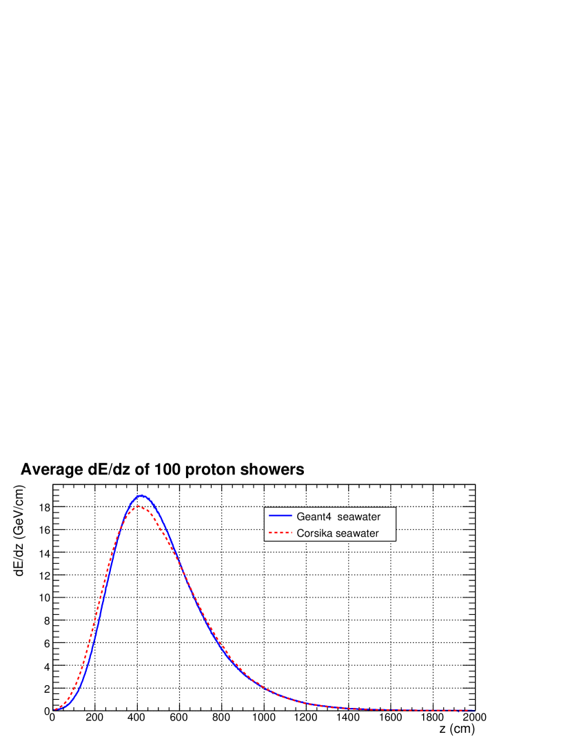
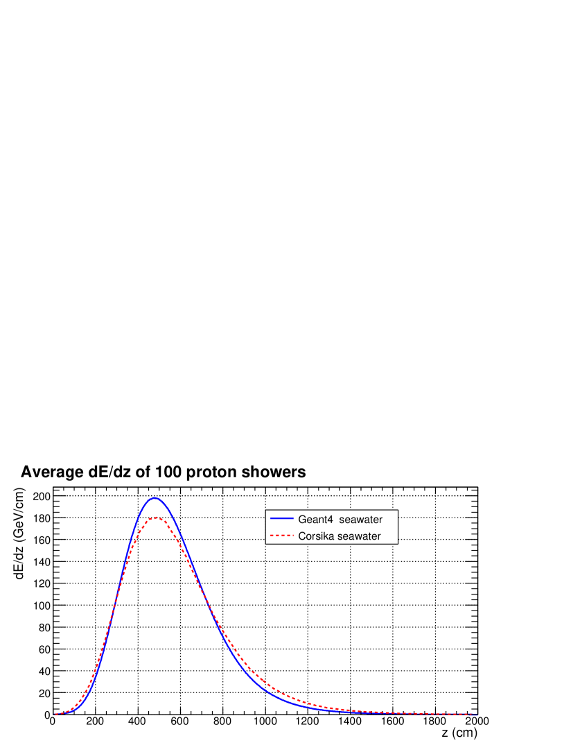
Figure 2: Averaged longitudinal energy deposited per unit path length of 100 proton showers at energy $10^{4}$ GeV (upper plot) and $10^{5}$ GeV (lower plot) generated in Geant4 and CORSIKA versus depth in the water.

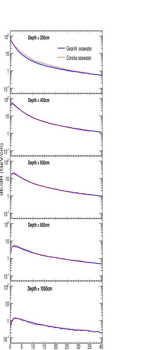
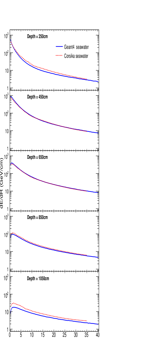
Figure 3: Averaged radial energy deposited per 20 g cm^-2 vertical slice per unit radial distance for 100 proton showers at energy $10^{4}$ GeV (left hand plots) and $10^{5}$ GeV (right hand plots) generated in Geant4 and CORSIKA versus distance from the axis in the water for different depths of the shower.

Figure 2 shows the longitudinal distributions of proton showers at energies of $10^{4}$ and $10^{5}$ GeV (averaged over 100 showers) as determined from Geant4 and CORSIKA. The showers from CORSIKA tend to be slightly broader and with a smaller peak energy than those generated by Geant4. The difference in the peak height is $\sim 5\%$ at $10^{4}$ GeV rising to $\sim 10\%$ at energy $10^{5}$ GeV. Figure 3 shows the radial distributions. The differences in the longitudinal distributions are reflected in the radial distributions. However, the shapes of the radial distributions are very similar between Geant4 and CORSIKA, with CORSIKA producing $\sim 10\%$ more energy near the shower axis at depths between 450 and 850 g cm^-2 where most of the energy is deposited. The acoustic signal from a shower is most sensitive to the radial distribution, particularly near the axis ($r\sim 0$). It is relatively insensitive to the shape of the longitudinal distribution.

3.2 Comparison with the simulation of Alvarez-Muñiz and Zas

The CORSIKA simulation was also compared with the longitudinal shower profile for protons computed in the simulation by Alvarez-Muñiz and Zas (AZ) [24]. There was a reasonable agreement between the longitudinal shower shapes from CORSIKA and those shown in Figure 2 of ref. [24]. However, the numbers of electrons and positrons at the peak of the CORSIKA showers was $\sim 20\%$ lower than those from ref. [24]. This number is sensitive to the energy below which these particles are counted and this is not specified in [24]. Hence the agreement between CORSIKA and their simulation is probably satisfactory within this uncertainty.

In conclusion, the modifications made to CORSIKA to simulate high energy showers in a water medium give results which are compatible with the predictions from the Geant4 simulations for energy less than $10^{5}$ GeV and the simulation of AZ within $20\%$. This is taken to be the accuracy of the simulation program assuming that there are no unexpected and unknown interactions between the centre of mass energy explored at current accelerators and those studied in these simulations. Studies of the sensitivity of the CORSIKA simulation to the different models of the hadronic interactions have been reported in reference [25]. They find that the peak number of electrons plus positrons varies by $\sim 20\%$ for proton showers in air depending on the choice of the hadron interaction model used. These differences are similar in magnitude to the differences between the AZ, Geant4 and CORSIKA simulations reported here. Hence the observed differences between the Geant4, AZ and CORSIKA simulations in water could be within the uncertainties of the hadronic interaction models.

4 Simulation of neutrino induced showers

Neutrinos interact with the nuclei of the detection medium by either the exchange of a charged vector boson ($W^{+}$), i.e. charged current (CC) interactions or the exchange of the neutral vector boson ($Z^{0}$), i.e. neutral current (NC) deep inelastic scattering interactions (see for example [26]). The ratio of the CC to NC interaction cross sections is approximately 2:1. The CC interactions produce charged secondary scattered leptons while the NC interactions produce neutrinos. The hadron shower carries a fraction $y$ of the energy of the incident neutrino and the scattered lepton the remaining fraction $1-y$. We assume that the neutrino flavours are homogeneously mixed when they arrive at the Earth by neutrino oscillations. Hence in the CC interactions electrons, $\mu$ and $\tau$ leptons will be produced as the scattered leptons in equal proportions. At the energies we shall consider, these particles behave in a manner similar to minimum ionising particles for $\mu$ and $\tau$ leptons. This is almost true also for electrons for which the bremsstrahlung process will be suppressed by the LPM effect. Hence the charged scattered leptons contribute little to the energy producing an acoustic signal. In the case of NC interactions there is no contribution to this energy from the scattered lepton. For these reasons the contribution of the scattered lepton to the shower profile is ignored beyond $z=20$ m in what follows.

It is interesting to note that a $\tau$ lepton can decay to hadrons or a very high energy electron or muon can produce bremsstrahlung photons at large distances from the interaction point. These can initiate further distant showers, the so called “double bang” effect. The stochastic nature of such electron showers is studied in [15, 16]. These effects are not considered in this study.

4.1 Neutrino-nucleon interaction cross sections.

A number of groups have computed the high energy neutrino-nucleon interaction cross sections, $\sigma$, [29, 27, 28]. In the quark parton model of the nucleon for the single vector boson exchange process, the differential cross section for CC interactions can be expressed in terms of the measured structure functions of the target nucleon $F_{2}$ and $xF_{3}$ as

$$\frac{d^{2}\sigma}{dQ^{2}dy}=\frac{G_{F}^{2}}{2\pi y}\bigg{(}\frac{M_{W}^{2}}{Q^{2}+M_{W}^{2}}\bigg{)}^{2}(F_{2}(x,Q^{2})(1-y+y^{2}/2)\pm y(1-y/2)xF_{3}(x,Q^{2}))$$ (1)

where $G_{F}$ is the Fermi weak coupling, $M_{W}$ is the mass of the weak vector boson, $Q^{2}$ is the square of the four momentum transferred to the target nucleon, $y=\nu/E$ where $\nu$ is the energy transferred to the nucleon ($\nu=E-E^{\prime}$ with $E$ and $E^{\prime}$ the energies of the incident and scattered leptons) and $x=Q^{2}/2M\nu$ is the fraction of the momentum of the target nucleon carried by the struck quark (here $x$ and $y$ are defined for a stationary target nucleon). The plus (minus) sign is for neutrino (anti-neutrino) interactions. It can be seen that $y$ is the fraction of the neutrino’s energy which is converted into the energy of the hadron shower. A similar expression can be written down for the NC interaction (see for example [26]) which has a ratio to the CC cross section varying from 0.33 to 0.41 as the neutrino energy increases from $10^{4}$ to $10^{13}$ GeV. The structure functions $F_{2}$ and $xF_{3}$ are the sum of the quark distribution functions which have been parameterised by fitting data [30, 31]. It can be shown that $Q^{2}=sxy$ where $s=2ME$ is the square of the centre of mass energy ($M$ is the target nucleon mass). To compute the cross sections the structure functions must be calculated at values of $x\lesssim M_{W}^{2}/s$ i.e. at values well outside the region of the fits to the parton distribution functions (PDFs) which have been performed for $x\gtrsim 10^{-5}$, the range of current measurements. The extrapolation outside the measurement range is discussed in [27], [29] and [32, 33]. Here we adopt the procedure of extrapolating linearly on a log-log scale from the parameterised parton distribution functions of [30] computed at $x=10^{-4}$ and $x=10^{-5}$. By considering various theoretical evolution procedures it is estimated in [29] that the procedure has an accuracy of $\sim 32\%$ per decade and we use this as an estimate of the accuracy of the calculation. However, this could be an underestimate [34].

The expression in equation 1 for charged current interactions and the one for neutral current interactions were integrated to obtain the total neutrino-nucleon interaction cross section, the value of the fraction of events per interval of $y$, $1/\sigma d\sigma/dy$, and the mean value of $y$. The total cross section was found to be in good agreement with the values in [27, 29] and in reasonable agreement with [28] which is based on a model different from the quark parton model. Figure 4 shows the mean value of $y$ obtained from this procedure (solid curve) and the effect of multiplying or dividing the PDFs by a factor 1.32 per decade (dashed curves) as an indication of the possible range of uncertainties in the extrapolation of the PDFs. Figure 5 shows the $y$ dependence of the cross section for different neutrino energies.

4.2 A simple generator for neutrino interactions.

A simple generator for neutrino interactions in a column of water of thickness 20 m was constructed as follows. The neutrino interacts at the top of the water column (z=0, with the z axis along the axis of the column). The energy fraction transferred, $y$, for the interaction was generated, distributed according to the curve for the energy of the neutrino shown in Figure 5. This allows the energy of the hadron shower to be calculated for the event. The assumption was made that these hadron showers will have approximately the same distributions as those of a proton interaction at z=0 (see Section 4.3 for a test of this assumption). A series of files of 100 such proton interactions were generated at energies in steps of half an order of magnitude between $10^{5}$ and $10^{12}$ GeV. The hadron shower for each neutrino interaction was selected at random from the 100 showers in the file at the proton energy closest to the energy of the hadron shower. The deposited energy in each bin was then multiplied by the ratio of the energy of the hadron shower to that of the proton shower. This is made possible because the shower shapes vary slowly with shower energy. For example, the ratio of the peak energy deposit per 20 g cm^-2 slice to the shower energy varies from 0.037 to 0.030 as the proton shower energy varies from $10^{5}$ to $10^{12}$ GeV.

4.3 The HERWIG neutrino generator.

The CORSIKA program has an option to simulate the interactions of neutrinos at a fixed point [35]. The first interaction is generated by the HERWIG package [36]. This option was adapted to our version of CORSIKA in sea water. Some problems were encountered with the $y$ dependence of the resulting interactions due to the extrapolation of the PDFs to very small $x$ at high energies. This only affects the rate of the production of the showers at different $y$ and the distribution of the hadrons produced in the interaction at a given $y$ should be unaffected.

A total of 700 neutrino interactions were generated at an incident neutrino energy of $2\cdot 10^{11}$ GeV. These were divided into the shower energy intervals $0.5-2\cdot 10^{10}$, $2-4\cdot 10^{10}$, $4-7.5\cdot 10^{10}$, $0.75-1.3\cdot 10^{11}$ and $1.3-2\cdot 10^{11}$. The showers in which the scattered lepton energy disagreed with the shower energy by more than $20\%$ were eliminated leading to a loss of $17\%$ of the events with shower energy greater than $0.5\cdot 10^{10}$ GeV. This is due to radiative effects and misidentification of the scattered lepton. Approximately 70 events remained in each energy interval. The energy depositions from these were averaged and compared to the averages from proton showers scaled by the ratio of the shower energy to the proton energy. Figure 6 shows the longitudinal distributions of the hadronic shower energy deposited for the different energy intervals (labelled $E_{W}$) compared to the scaled proton distributions. Figure 7 shows a sample of the transverse distributions.

There is a good consistency between the proton and neutrino induced showers. The proton showers peak, on average, 20 g cm^-2 shallower in depth with a peak energy $2\%$ larger than the neutrino induced showers. This is small compared to the overall uncertainty. The slight shift in the longitudinal distribution is reflected as a normalisation shift in the radial distributions. We conclude therefore that to equate a proton induced shower starting at the neutrino interaction point to that from a neutrino is a satisfactory approximation.

5 Parameterisation of showers

In this section a parameterisation of the energy deposited by the showers generated by CORSIKA (averaged over 100 showers depositing the same total energy) is described. Other available parameterisations will then be compared with the showers generated by CORSIKA.

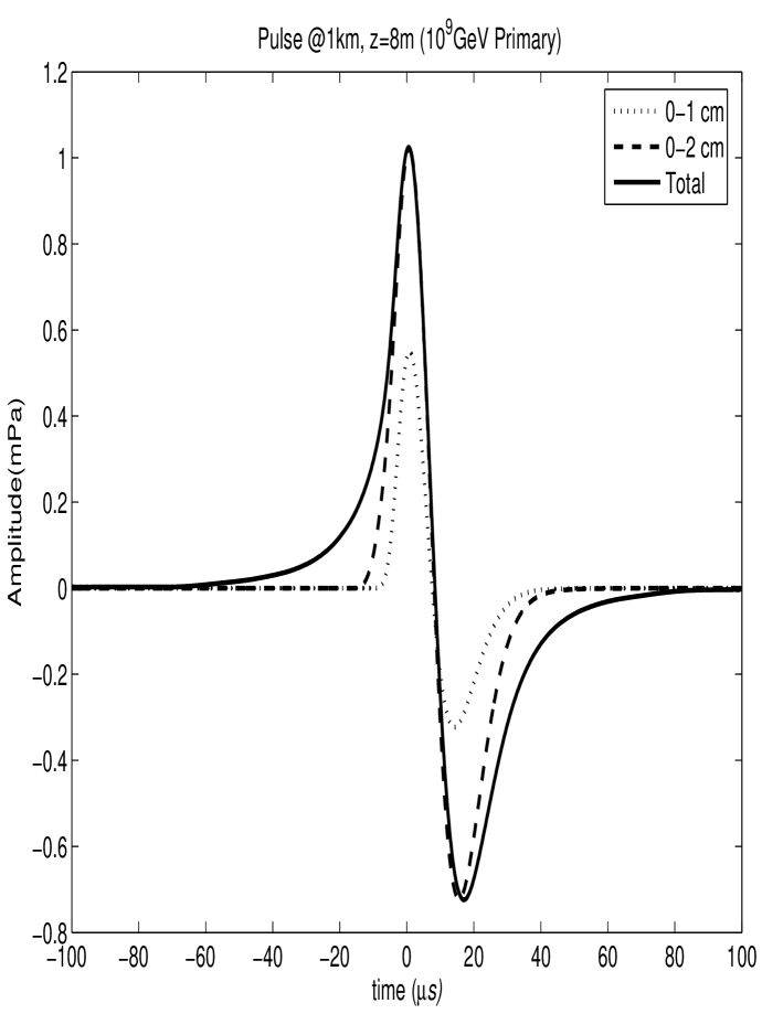
Figure 8: The acoustic signal at a distance of 1 km from the shower axis in the median plane computed from the average of 100 CORSIKA showers each depositing a total energy of $10^{9}$ GeV in the water. The dotted, dashed and solid curves shows the signals computed from the deposited energies within cores of radius 1.025 g cm^-2, 2.05 g cm^-2 and the whole shower (solid curve), respectively. It can be seen that most of the amplitude of the signal comes from the energy within a core of radius 2.05 g cm^-2.

The acoustic signal generated by a hadron shower depends mainly on the energy deposited in the inner core of the shower. This is illustrated in figure 8 which shows the contribution to the acoustic signal from cores of different radii. This figure shows that it is crucial to represent the deposited energy well at radius less than 2.05 g cm^-2. The calculation of the acoustic signal from the deposited energy is described in section 6.

5.1 Parameterisation of the CORSIKA Showers

The differential energy deposited was parameterised as follows

$$\frac{d^{2}E}{drdz}=L(z,E_{L})\cdot R(r,z,E_{L})$$ (2)

where the function $L(z,E_{L})$ represents the longitudinal distribution of deposited energy and $R(r,z,E_{L})$ the radial distribution. Here $E_{L}$ is $\log_{10}E$ with $E$ the total shower energy.

The function $L(z,E_{L})=dE/dz$ is a modified version of the Gaisser-Hillas function [37]. This function represents the longitudinal distribution of the energy deposited.

$$L(z,E_{L})=P_{1L}\bigg{(}\frac{z-P_{2L}}{P_{3L}-P_{2L}}\bigg{)}^{\frac{(P_{3L}-P_{2L})}{P_{4L}+P_{5L}z+P_{6L}z^{2}}}\exp\bigg{(}{\frac{P_{3L}-z}{P_{4L}+P_{5L}z+P_{6L}z^{2}}}\bigg{)}$$ (3)

Here the parameters $P_{nL}$ were fitted to quadratic functions of $E_{L}=\log_{10}E$ with values

$$\frac{P_{1L}}{E}=2.760\cdot 10^{-3}-1.974\cdot 10^{-4}E_{L}+7.450\cdot 10^{-6}E_{L}^{2}$$ (4)

$$P_{2L}=-210.9-6.968\cdot 10^{-3}E_{L}+0.1551E_{L}^{2}$$ (5)

$$P_{3L}=-41.50+113.9E_{L}-4.103E_{L}^{2}$$ (6)

$$P_{4L}=8.012+11.44E_{L}-0.5434E_{L}^{2}$$ (7)

$$P_{5L}=0.7999\cdot 10^{-5}-0.004843E_{L}+0.0002552E_{L}^{2}$$ (8)

$$P_{6L}=4.563\cdot 10^{-5}-3.504\cdot 10^{-6}E_{L}+1,315\cdot 10^{-7}E_{L}^{2}.$$ (9)

The parameter $P_{1L}$ represents the peak energy deposited and $P_{3L}$ the depth in the $z$ coordinate at this peak while $P_{2L}$, $P_{4L}$, $P_{5L}$ and $P_{6L}$ are related to the shower width and shape in $z$.

The radial distribution was represented by the NKG function [37]

$$R(r,z,E_{L})=\frac{1}{I}\bigg{(}\big{(}\frac{r}{P_{1R}}\big{)}^{(P_{2R}-1)}\big{(}1+\frac{r}{P_{1R}}\big{)}^{(P_{2R}-4.5)}\bigg{)}$$ (10)

where the integral

$$I=\int_{0}^{\infty}\bigg{(}\big{(}\frac{r}{P_{1R}}\big{)}^{(P_{2R}-1)}\big{(}1+\frac{r}{P_{1R}}\big{)}^{(P_{2R}-4.5)}\bigg{)}~{}dr=P_{1R}\frac{\Gamma(4.5-2P_{2R})\Gamma(P_{2R})}{\Gamma(4.5-P_{2R})}.$$

The parameter $P_{1R}$ was found to vary strongly with depth while $P_{2R}$ was only a weak function of depth. The parameters $P_{nR}$ (with $n=1$,$2$) were each represented by the quadratic form

$$P_{nR}=A+Bz+Cz^{2}$$ (11)

and the quantities $A,B,C$ parameterised as quadratic functions of $E_{L}$. This gave for $P_{1R}$

$$A=0.01287E_{L}^{2}-0.2573E_{L}+0.9636$$ (12)

$$B=-0.4697\cdot 10^{-4}E_{L}^{2}+0.0008072E_{L}+0.0005404$$ (13)

$$C=0.7344\cdot 10^{-7}E_{L}^{2}-1.375\cdot 10^{-6}E_{L}+4.488\cdot 10^{-6}$$ (14)

and for the parameter $P_{2R}$

$$A=-0.8905\cdot 10^{-3}E_{L}^{2}+0.007727E_{L}+1.969$$ (15)

$$B=0.1173\cdot 10^{-4}E_{L}^{2}-0.0001782E_{L}-5.093\cdot 10^{-6}$$ (16)

$$C=-0.1058\cdot 10^{-7}E_{L}^{2}+0.1524\cdot 10^{-6}E_{L}-0.1069\cdot 10^{-8}.$$ (17)

The fit was made in a depth range where $dE/dz$ was greater than $10\%$ of the peak value defined by equation 4. The program MINUIT [38] was used to minimise the squared fractional deviations

$$\chi^{2}=\sum_{i}\bigg{(}\frac{F_{i}-D_{i}}{F_{i}+D_{i}}\bigg{)}^{2}$$ (18)

where $F_{i}$ and $D_{i}$ refer to the fitted value and the value observed in the $i$th bin from the CORSIKA showers, respectively. In order to improve the fit at small radii the contributions to $\chi^{2}$ were arbitrarily weighted by 10 for $r<2.05$ g cm^-2, 4 for $2.05<r<3.075$ g cm^-2, unity for $3.075<r<51.25$ g cm^-2 and 0.25 for $r>51.25$ g cm^-2. The RMS value of the fractional deviations was $3.4\%$ for radii less than 51.25 g cm^-2 and for energies greater than $10^{6.5}$ GeV. The fit becomes poorer at lower energies and greater radii than these. Integrating the parameterisation shows that the fraction of the total energy computed from the fit within the fit range was $91\%$ averaged over the deposited energy range $10^{7}$ to $10^{12}$ GeV. The corresponding fraction directly from the CORSIKA distributions was $92.5\%$, averaged over the same energy range. When applying this parameterisation at depths with smaller energy deposit than $10\%$ of the peak value, the energy was assumed to be confined to an annular radius of 1.025 g cm^-2. There was a good agreement (within $5\%$ at the peak) between the acoustic signal computed using this parameterisation and that taken directly from the CORSIKA showers.

5.2 The parameterisation used by the SAUND Collaboration

The SAUND Collaboration [39] uses the following parameterisation [40], based on the NKG formulae (e.g. see reference [37]), for the energy deposited per unit depth, $z$, and per unit annular thickness at radius $r$ from a shower of energy $E$

$$\frac{d^{2}E}{drdz}=Ek(\frac{z}{z_{max}})^{t}\exp{(t-z/\lambda)}~{}2\pi r\rho(r)$$ (19)

where $z_{max}=0.9X_{0}\ln(E/E_{c})$ is the maximum shower depth, $X_{0}=36.1$ g cm^-2 is the radiation length and $E_{c}=0.0838$ GeV. The constants $t=z_{max}/\lambda$ where $\lambda=130-5\log_{10}(E/10^{4}\mathrm{GeV})$ g cm^-2 and $k=t^{t-1}/\exp{(t)}\lambda\Gamma(t)$. The radial density is given by

$$\rho(r)=\frac{1}{r_{M}^{2}}a^{s-2}(1+a)^{s-4.5}\frac{\Gamma(4.5-s)}{2\pi\Gamma(s)\Gamma(4.5-2s)}$$ (20)

where $a=r/r_{M}$ with $r_{M}=9.04$ g cm^-2, the Molière radius in water, and $s=1.25$. Figure 9 shows the radial distributions from CORSIKA compared with the absolute predictions of this parameterisation.

There is qualitative agreement between the parameterisation and the CORSIKA results. The difference in normalisation is explained by the somewhat different longitudinal profiles of the CORSIKA showers from the SAUND parameterisation. The latter are broader with a lower peak energy deposit and a depth of the maximum which is larger than the CORSIKA showers. CORSIKA predicts more energy at small $r$ than the SAUND parameterisation. Quantitatively, $51\%$ of the shower energy is contained within a cylinder of radius 4 cm for the CORSIKA showers compared to $35\%$ from the SAUND parameterisation. These fractions are approximately independent of energy. Hence, in acoustic detectors a harder frequency spectrum for the acoustic signals is predicted by CORSIKA than by the SAUND parameterisation. Note that in the fit described in Section 5.1 the values of the parameter $P_{1R}$ (equivalent to $R_{M}$ in equation 20) were strongly depth dependent and much lower than the Molière radius in water, assumed by the SAUND collaboration. In addition, the value of $P_{2R}$ (equivalent to $s$ in equation 20) while relatively constant tended to be at a higher value ($\sim 1.9$) than that assumed by SAUND.

5.3 The parameterisation used by Niess and Bertin

Hadron showers, generated by Geant4 (version 4.06 p03), were studied up to energies of $10^{5}$ GeV and electromagnetic showers to higher energies by Niess and Bertin [15, 16]. The hadronic showers were parameterised as follows.

$$\frac{d^{2}E}{drdz}=rf(z)g(r,z)$$ (21)

with

$$f(z)=\frac{E}{X_{0}}b\frac{(bz^{\prime})^{a-1}\exp{-bz^{\prime}}}{\Gamma(a)}$$ (22)

where $E$ is the energy of the hadron shower, $X_{0}$ is the radiation length in water, $z^{\prime}=z/X_{0}$, $b=0.56$ as determined from the fit and $a$ is chosen to satisfy $z_{max}^{\prime}=(a-1)/b$. Here $z_{max}^{\prime}$ is the depth in radiation lengths at which the shower maximum occurs. This is parameterised as

$$z_{max}^{\prime}=0.65\log(\frac{E}{E_{c}})+3.93$$ (23)

with $E_{c}=0.05427$ GeV. The radial distribution function is parameterised as

$$g(r,z)=g_{0}\bigg{(}\frac{r_{i}}{r}\bigg{)}^{n}$$ (24)

where $r_{i}=3.5$ cm, $n=n_{1}=1.66-0.29(z/z_{max})$ for $r<r_{i}$ and $n=n_{2}=2.7$ for $r>r_{i}$. The constant $g_{0}$ is chosen to be $(2-n_{1})(n_{2}-2)/((n_{2}-n_{1})r_{i}^{2})$ so that the integral of the radial distribution is unity.

Figure 10 shows the radial distributions from this parameterisation compared with the predictions of CORSIKA. There is quite good agreement between the two. There is a difference in the normalisation with depth since Geant4, on which this parameterisation is based, produces showers which tend to develop more slowly with depth than those from CORSIKA (see Figure 2). Furthermore, both this and the SAUND parameterisation (Section 5.2) assume a linear variation of the shower peak depth with $\log E$ whereas CORSIKA gives a clear parabolic shape (see equation 6). This is illustrated in Figure 11. The Niess-Bertin parameterisation predicts that $56\%$ of the shower energy is contained within a cylinder of radius 4 cm in reasonable agreement with the value of $51\%$ from CORSIKA (these values are almost independent of energy).

6 The acoustic signals from the showers.

The pressure, $P$, from a hadron shower depositing total energy $E$ at time $t$ resulting from the deposition of relative energy density $\epsilon=(1/E)(1/2\pi r)d^{2}E/drdz$ at a point distant $d$ from the volume, $dV$, follows the form [13]

$$P(d,t)=\frac{E\beta}{4\pi C_{p}}\int\frac{\epsilon}{d}\frac{d}{dt}\bigg{(}\delta(t-d/c)\bigg{)}dV$$ (25)

where the integral is over the total volume of the shower. Here $\beta=2.0\cdot 10^{-4}$ is the thermal expansion coefficient of the medium at $14^{\circ}$C, $C_{p}=3.8\cdot 10^{3}$ J kg^-1 K^-1 is the specific heat capacity and $c=1500$ ms^-1 is the velocity of sound in the sea water.

Acoustic signals seen by an observer at distance $r$ from the shower centre are computed from equation (25) as follows. Points are produced randomly throughout the volume of the shower with density proportional to the deposited energy density and the time of flight from every produced point to the observer calculated. The flight times to the observer are histogrammed over $2^{n}$ bins (in this case $n=10$ is chosen) centred on the mean flight time and with a suitable bin width, $\tau$ (chosen here to be 1$\mu$s). The counts in each bin of the histogram are divided by $\tau$ yielding the function $E_{xyz}(t)$. The Fourier transform of the pressure wave is then

$$P(\omega)=\frac{1}{r}\int_{-\infty}^{\infty}\frac{E\beta}{4\pi C_{p}}\frac{d}{dt}E_{xyz}(t)e^{-i\omega t}dt=\frac{1}{r}\frac{E\beta}{4\pi C_{p}}i\omega\int_{-\infty}^{\infty}E_{xyz}(t)e^{-i\omega t}dt=\frac{1}{r}\frac{E\beta}{4\pi C_{p}}i\omega E_{xyz}(\omega)$$ (26)

using the standard Fourier transform theorem, that taking the derivative in the time domain is the same as multiplying by $i\omega$ in the frequency domain. The Fourier transform $E_{xyz}(\omega)$ at angular frequency $\omega$ is evaluated numerically by a fast Fourier Transform (FFT) from the histogram $E_{xyz}(t)$. A correction is applied for attenuation in the water by a factor $A(\omega)=e^{-\alpha(\omega)r}$ where $\alpha(\omega)$ is the frequency dependent attenuation coefficient. The pressure as a function of time is then evaluated numerically by an inverse FFT using frequency steps from zero to the sampling frequency (the inverse of the bin width $\tau$ i.e. 1 MHz in this case). This gives

$$P(t)=\frac{1}{1024}\sum_{n=-512}^{n=511}P(\omega_{n})A(\omega_{n})e^{in\Omega}$$ (27)

where $\Omega=2\pi/1024$ radians and $\omega_{n}/2\pi=n\Omega/2\pi$ MHz is the $n$th frequency. The attenuation coefficient $\alpha(\omega)$ is computed either according to the formulae in [42] or using the complex attenuation given in [15, 16]. This method of calculation was computationally much faster than the evaluation of the space integral given in equation 18 of reference [13] and gave identical results.

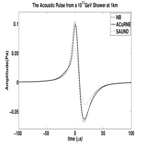
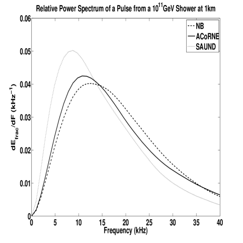
Figure 12: The left hand plot shows acoustic pulses generated from the parameterisation described in section 5.1 labelled ACoRNE, the parameterisation from reference [15, 16] labelled NB and that from reference [39, 40] labelled SAUND. These pulses were evaluated for a hadron shower from a neutrino interaction depositing hadronic energy of $10^{11}$ GeV 1 km distant from an acoustic detector in a plane perpendicular to the shower axis at the shower maximum (the median plane). The right hand plot shows the frequency decomposition of the pulses in the left hand plot.

Acoustic pulses, computed with the complex attenuation described in [15, 16], using the parameterisations of the shower profile given above are shown in Figure 12. It can be seen that the parameterisation developed here gives similar results to that described in [15, 16] despite the fact that the latter was an extrapolation from low energy simulations. The parameterisation used by SAUND [39, 40] gives smaller signals concentrated at somewhat lower frequencies.

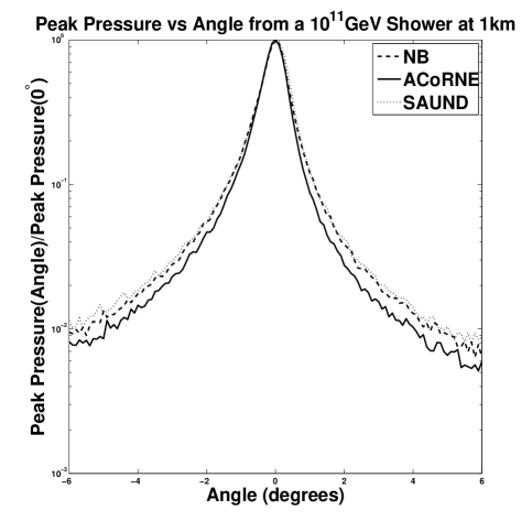
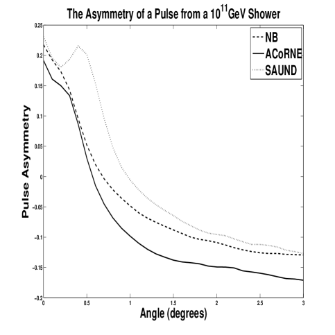
Figure 13: The left hand plot shows the variation of the peak pressure in the pulse with angle from the median plane at 1 km from the shower. The right hand plot shows the variation of the pulse asymmetry with this angle at the same distance. The curves were computed from the parameterisations labelled.

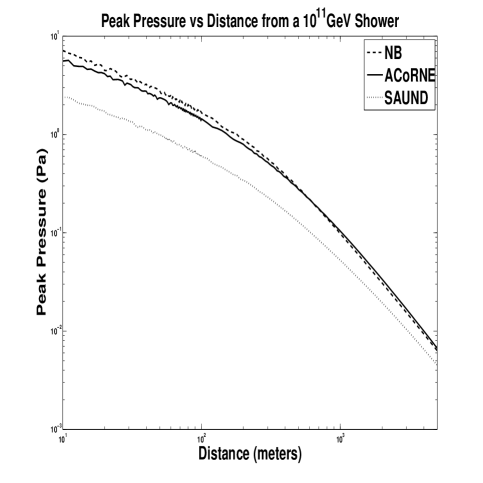
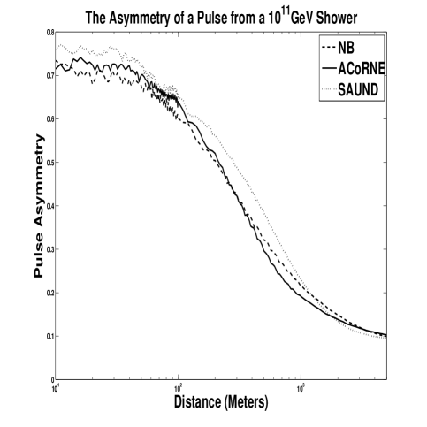
Figure 14: The left hand plot shows the decrease of the pulse peak pressure and the right hand plot the pulse asymmetry, both in the median plane, as a function of distance from the shower computed from the parameterisations.

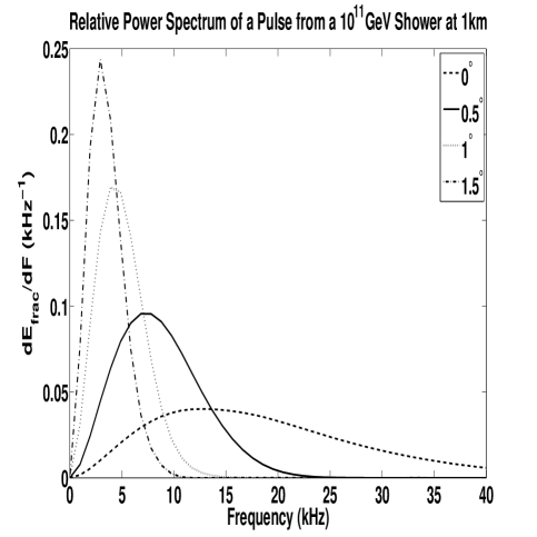
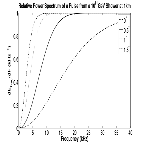
Figure 15: The left hand plot shows the frequency decomposition of the acoustic signal, computed from the parameterisation of the CORSIKA showers, at different angles to the median plane at a distance of 1km from the shower and the right hand plot shows the cumulative frequency spectrum i.e. the integral of the left hand plot.

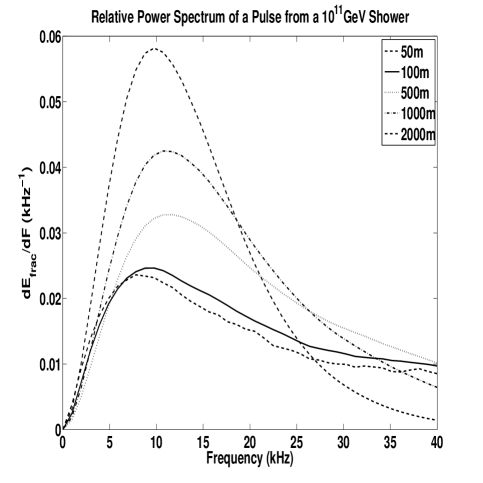
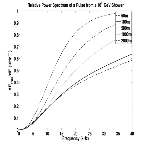
Figure 16: The left hand plot shows the frequency decomposition of the acoustic signal, computed from the parameterisation of the CORSIKA showers, at different distances from the hydrophone in the median plane and the right hand plot shows the cumulative frequency spectrum i.e. the integral of the left hand plot.

Further properties of the acoustic signals are shown in Figures 13 to 16. The pulses tend to be somewhat asymmetric with the asymmetry defined by $|P_{max}|-|P_{min}|/|P_{max}|+|P_{min}|$. The complex nature of the attenuation enhances this asymmetry. This is most evident in the far field conditions e.g. at 5km where non complex attenuation would yield a totally symmetric pulse. Figure 13 shows the angular dependence of the peak pressure. Here the angle is that subtended by the acoustic detector relative to the plane, termed the median plane, through the shower maximum at right angles to the axis of the shower. The parameterisation derived here gives a somewhat narrower angular spread than the others. This could be due to the slightly longer showers predicted by CORSIKA than the others. Figure 13 also shows the asymmetry of the pulse as a function of this angle. The pulse initially becomes more symmetric moving out of the median plane and then the asymmetry becomes negative at larger angles. Figure 14 shows the decrease of the pulsed peak pressure with distance from the shower in the median plane and the asymmetry with distance in this plane. Figures 15 and 16 show the frequency composition of the pulses at different angles to the median plane at 1 km from the shower and at different distance in the median plane, respectively.

7 Conclusions

The simulation program for high energy cosmic ray air showers, CORSIKA, has been modified to work in a water or ice medium. This allows both hadron and neutrino showers to be generated in the medium over a wide range of energy ($10^{5}$ to $10^{12}$ GeV). The properties of hadronic showers in water simulated by CORSIKA agree with those from other simulations to within $10-20\%$. A similar uncertainty has been noted previously from the variations in CORSIKA showers in air generated by different models of the hadron interactions. However, none of the other available simulations for water cover the range of energies accessible to CORSIKA. The hadronic showers produced by neutrino interactions are shown to have similar profiles to proton showers which deposit the same amount of energy to that from the neutrino and which start at the interaction point of the neutrino. The properties of the neutrino interactions are described. A parameterisation of the shower profiles generated by CORSIKA is given. There is reasonable agreement with the parameterisation based on the Geant4 simulations at low energy ($<10^{5}$ GeV) developed by Niess and Bertin. However, the agreement with the parameterisation used by the SAUND Collaboration, which is based on the NKG formalism, is less good. The position of the shower maximum, determined from the CORSIKA program, is found to vary quadratically with $\log E$ rather than linearly as assumed in the latter two parameterisations.

The acoustic signals generated by neutrino interactions using CORSIKA and by the two other parameterisations are described and their properties are studied. The acoustic signal is found to be very sensitive to the energy deposited close to the shower axis.

7.1 Acknowledgments

We wish to thank Ralph Engel, Dieter Heck, Johannes Knapp and Tanguy Pierog for their assistance in modifying the CORSIKA program. We also thank Valentin Niess and Justin Vandenbroucke for valuable discussions.

Figure 1: The interaction length for high energy gamma rays versus the photon energy measured in CORSIKA (data points with statistical errors). The dash dotted curve shows the pair production length computed from the LPM effect using the formulae of Migdal [19]. The solid curve shows the computed total interaction length, including both pair production and photonuclear interactions with the cross section from CORSIKA. The dashed line labelled $9/7X_{0}$ shows the expected pair production length without the LPM effect. Here $X_{0}$ is the radiation length of the material.

Figure 4: The mean value of $y$ as a function of energy for $\nu_{\mu}$ interactions computed according to the standard model with the PDFs of MRS99 [30], extrapolating $x$ and $Q^{2}$ out of the fit range from $x=10^{-4}$ linearly on a log-log scale. The upper dashed curve shows the result of multiplying the PDFs by $1.32^{\log(10^{-4}/x)}$ for PDFs with $x<10^{-4}$ and the lower dashed curve by dividing by this factor. The deviations of the dashed curve from the solid one is an indication of the precision of the standard model.

Figure 5: The fraction of events per unit $y$ interval for different $\nu_{\mu}$ energies computed by integrating the expressions for the CC and NC cross sections.

Figure 6: The longitudinal distribution of the deposited energy for neutrino showers (solid) generated by the Herwig-CORSIKA package and proton showers (dashed) scaled to the same values of shower energy $E_{W}$. The scaling factors applied to the average of the protons showers with energy $10^{10}$ GeV were 1.0 and 3.0 for $E_{W}=10^{10}$ GeV and $E_{W}=3\cdot 10^{10}$ GeV, respectively. Those applied to proton showers with energy $10^{11}$ GeV were 0.575, 1.0 and 1.65 for $E_{W}=5.75\cdot 10^{10}$ $E_{W}=10^{11}$ and $E_{W}=1.65\cdot 10^{11}$ GeV, respectively.

Figure 7: The solid curves show the averaged radial energy deposited per 20 g cm^-2 vertical slice per unit radial distance for 70 neutrino showers with energy transfer $E_{W}=3\cdot 10^{10}$ GeV (left hand plots) and $E_{W}=1.65\cdot 10^{11}$ GeV (right hand plots). The incident neutrino energy was $2\cdot 10^{11}$ GeV. For comparison the dashed curves show the distributions from proton showers scaled to these energies. In the left (right) hand plots protons of energy $10^{10}$ GeV ($10^{11}$ GeV) were scaled by a factor of 3 (1.65).

Figure 9: The radial distributions of the deposited energy at different depths from CORSIKA compared to the parameterisation used by the SAUND collaboration [39] for $10^{6}$ GeV and $10^{11}$ GeV proton induced showers.

Figure 10: The radial distributions of the deposited energy at different depths from CORSIKA compared to the parameterisation used by the Niess and Bertin [16, 15] (labelled NB parameterisation) for $10^{6}$ GeV and $10^{11}$ GeV proton induced showers.

Figure 11: The depth of the shower peak as a function of $\log_{10}E$ from CORSIKA (black points) for the showers starting at $z=0$. The solid curve shows the parameterisation according to equation 6. The dashed (dash dotted) lines show the values assumed by the SAUND (Niess-Bertin) Collaborations.

References

- [1] Proceedings of the Workshop on Acoustic and Radio EeV Neutrino Detection Activities (ARENA), DESY, Zeuthen (May 2005), Editors R. Nahnhauer and S. Böser
-
[2]
K. Griesen, Phys. Rev. Lett.16 (1966) 748,
G.T. Zaptsepin, V.A. Kuzmin, JETP Lett. 4 (1966) 78. - [3] E. Waxman and J. Bahcall, Phys. Rev. D59 (1999) 023002, (hep-ph/9807282).
- [4] R.D. Engel, D. Seckel and T.Stanev, Phys. Rev. D64 (2001) 093010 (astro-ph/0101216).
- [5] See for example M. Ackermann et al., (astro-ph/0412347) Phys. Rev. D71 (2005) 077102.
- [6] See for example Nucl. Instrum. Meth. A567 (2006) 438
- [7] J.A. Aguilar et al., astro-ph/0606229.
- [8] See for example G. Aggouras et al., Nucl. Instrum. and Meth. A552 (2005) 420.
- [9] See for example Nucl. Phys. Proc. Suppl. 143 (2005) 373.
- [10] “CORSIKA: A Monte Carlo Code to Simulate Extensive Air Showers”, D. Heck et al., Karlsruhe Report FZKA 6019. (http://www-ik.fzk.de/corsika).
- [11] G. Askar’yan, Soviet Physics JETP 14 (1962) 441 and 21 (1965) 658.
- [12] J. Alvarez-Muñiz, E. Marqués, R.A. Vázquez and E. Zas Phys. Rev. D68 (2003) 043001 (astro-ph/0206043).
- [13] J.G. Learned Phys. Rev. D19 (1979) 3293.
- [14] J. Alvarez-Muñiz and E.Zas, Phys. Lett. B434 (1998) 396 (astro-ph/9806098).
- [15] V. Niess and V. Bertin astro-ph/0511617 and V. Niess, PhD Thesis, CPPM, Marseille.
- [16] V. Niess, PhD Thesis, CPPM, Marseille, see equations 1-55 and 1-56.
- [17] Geant4, J. Allison et al., Nucl. Inst. and Meths. in Phys. Research A506 (2003) 250 and IEEE Transactions on Nucl. Science 53 (2006) 270.
- [18] “The EGS4 Code System” W.R. Nelson, H.Hirayama and D.W.O. Rogers, report number SLAC-265.
-
[19]
L.D. Landau and I.J. Pomeranchuk, Dokl. Akad. Nauk. SSSR
92 (1953) 535 and 92 (1953) 735. These papers are available in
English in L. Landau, “The Collected Papers of L.D. Landau”, Pergamon Press 1965.
A.B. Migdal, Phys. Rev. 103 (1956) 1811. - [20] Particle data table, Phys. Lett. 592 (2004) 1.
- [21] R. M. Sternheimer, S.M. Seltzer and M.J.Berger, Atomic Data and Nuclear Data Tables 30 (1984) 261.
- [22] D. Heck et al., Forschungszentrum Karlsruhe GmbH, Karlsruhe, Report number FZKA 6019 (1998).
- [23] N.N. Kalmykov and S. Ostapchenko, Phys. Atom. Nucl. 56 (1993) 346, N.N. Kalmykov et al., Nucl. Phys. Proc. Suppl. 52B (1997) 17.
- [24] J. Alvarez-Muniz and E. Zas, Phys. Lett. B434 (1998) 396 (astro-ph/9806098).
- [25] Influence of Hadronic Interaction Model on the Development of EAS in Monte Carlo Simulations, D. Heck, J.Knapp and G. Schatz, Nucl. Phys. B (Proc. Suppl.) 52B (1997) 139-141.
- [26] “An Introduction to the Physics of Quarks and Leptons” by P. Renton (published by Cambridge University Press, 1990)
- [27] J. Kwiecinski, A.D. Martin and A.M. Stasto Acta Phys. Polon. B31 (2000) 1273 (hep-ph/0004109).
- [28] A.Z. Gazizov and S.I. Yanush Phys. Rev. D65 (2002) 093003 (hep-ph/0105368)
- [29] R. Ghandi, C. Quigg, M.H. Reno, I. Sarcevic, Astroparticle Physics 5 (1996) 81.
- [30] A.D. Martin, R.G. Roberts, W.J.Stirling and R.S. Thorne, Eur. Phys. J. C14 (2000) 133 (hep-ph/9907231).
- [31] http://www.phys.psu.edu/ cteq/
- [32] J. Kwiecinski, A.D. Martin and A.M. Stasto, Phys. Rev. D59 (1999) 093002.
- [33] A.D. Martin, M.G.Ryskin and A.M. Stasto, Acta Phys. Polon. B34 (2003)3273.
- [34] R.S. Thorne, private communication.
- [35] O. Pisanti, private communication, see also M. Ambrosio et al., astro-ph/0302062.
- [36] HERWIG, G. Corcella et al., hep-ph/0011363.
- [37] “Introduction to Ultra High Energy Cosmic Rays” by P. Sokolsky (published by Addison-Wesley, 1989).
- [38] F. James and M. Roos, “Minuit, A System for Function Minimization and Analysis of the Parameter Errors and Correlations”, Comput. Phys. Commun. 10 (1975) 343.
- [39] J. Vandenbroucke, G. Gratta, N. Lehtenin, Astrophys. J. 621 (2005) 301. (astro-ph/0406105).
- [40] J. Vandenbroucke, private communication.
- [41] N.G. Lehtinen, S. Adam, G.Gratta, T.K. Berger and M.J. Buckingham (astro-ph/0104033).
- [42] M.A. Ainslie and J.G. McColm, J.Acoust. Soc. Am 103 (1998) 1671.