Modal Extraction in Spatially Extended Systems

Abstract

We describe a practical procedure for extracting the spatial structure and the growth rates of slow eigenmodes of a spatially extended system, using a unique experimental capability both to impose and to perturb desired initial states. The procedure is used to construct experimentally the spectrum of linear modes near the secondary instability boundary in Rayleigh-Bénard convection. This technique suggests an approach to experimental characterization of more complex dynamical states such as periodic orbits or spatiotemporal chaos.

Numerous nonlinear nonequilibrium systems in nature and in technology exhibit complex behavior in both space and time ; understanding and characterizing such behavior (spatiotemporal chaos) is a key unsolved problem in nonlinear science cross . Many such systems are modelled by partial differential equations; hence, in principle, their dynamics takes place in an infinite dimensional phase space. However, dissipation often acts to confine these systems’ asymptotic behavior to finite-dimensional subspaces known as invariant manifolds manneville . Knowledge of the invariant manifolds provides a wealth of dynamical information; thus, devising methodologies to determine invariant manifolds from experimental data would significantly advance understanding of spatiotemporal chaos.

In this Letter, we describe experiments in Rayleigh-Bénard convection where several slow eigenmodes and their growth rates associated with instability of roll states are extracted quantitatively. Rayleigh-Bénard convection (RBC) serves well as a model spatially extended system; in particular, the spiral defect chaos (SDC) state in RBC is considered an outstanding example of spatiotemporal chaos. In SDC the spatial structure is primarily composed of curved but locally parallel rolls, punctuated by defects (Fig. 1) morris ; egolf1 . The recurrent formation and drift of defects in SDC is believed to play a key role in driving spatiotemporal chaos; moreover, many aspects of defect nucleation in SDC are related to defect formation observed at the onset of instability in patterns of straight, parallel rolls in RBC busse . We obtain experimentally a low-dimensional description of the modes responsible for the nucleation of one important class of defects (dislocations), by first imposing reproducibly a linearly stable, straight roll state (stable fixed point) near instability onset. This state is subsequently subjected to a set of distinct, well-controlled perturbations, each of which initiates a relaxational trajectory from the disturbed state to the (same) fixed point. An ensemble of such trajectories is used to construct a suitable basis for describing the embedding space by means of a modified Karhunen-Loeve decomposition. The dynamical evolution of small disturbances is then characterized by computing both finite-time Lyapunov exponents and the spatial structure of the associated eigenmodes (a similar approach was carried out numerically by Egolf et al. egolf2 ). This capability is an important step toward developing a systematic way of characterizing and, perhaps, controlling, spatiotemporally chaotic states like SDC where localized “pivotal” events like defect formation play a central role in driving complex behavior.

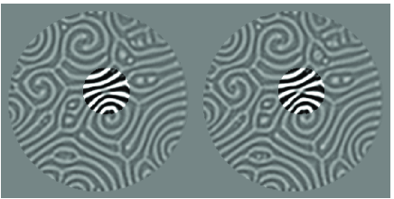
Figure 1: Shadowgraph visualization reveals spontaneous defect nucleation in the spiral defect chaos state of Rayleigh-Benard convection. Two convection rolls are compressed together (higher contrast region in left image). (b.) A short time later (right image), one of the rolls pinches off and two dislocations form.

The convection experiments are performed with gaseous CO₂ at a pressure of 3.2 MPa. A 0.697$\pm$0.06 mm-thick gas layer is contained in a 27 mm square cell, which is confined laterally by filter paper. The layer is bounded on top by a sapphire window and on the bottom by a sheet of 1 mm-thick glass neutral density filter(NDF). The neutral density filter is bonded to a heated metal plate with heat sink compound. The temperature of the sapphire window held constant at 21.3 ^∘C by water cooling. The temperature difference between the top and bottom plates $\Delta T$ is held fixed at 5.50 $\pm$ 0.01 ^∘C by computer control of a thin film heater attached to the bottom metal plate. These conditions correspond to a dimensionless bifurcation parameter $\epsilon$=$(\Delta T-\Delta T_{c})/\Delta T_{c}=0.41$, where $\Delta T_{c}$ is the temperature difference at the onset of convection. The vertical thermal diffusion time, computed to be 2.1 s at onset, represents the characteristic timescale for the system.

We use laser heating to alter the convective patterns that occur spontaneously. A focused beam from an Ar-ion laser is directed through the sapphire window at a spot on the NDF. Absorption of the laser light by the NDF increases the local temperature of the bottom boundary and hence that of the gas, thereby inducing locally a convective upflow. The convection pattern may be modifed, either locally or globally, by rastering the hot spot created by the laser beam. The beam is steered using two galvanometric mirrors rotating about axes orthogonal to each other under computer control. The intensity of the beam is modulated using an acousto-optic modulator. This technique of optical actuation is used to impose convection patterns with desired properties, to perturb these convection patterns and to change the boundary conditions. Similar approaches for manipulating convective flows were explored earlier using a high intensity lamp and masks whitehead in RBC and a rastered infrared laser in Bénard-Marangoni convection denis .

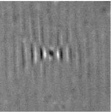
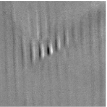
Figure 2: Experimental images illustrate the flow response to two different perturbations applied, in turn, to the same state of straight convection rolls. Each image represents the difference between the perturbed and unperturbed convection states and therefore, each image highlights the effect of a given perturbation on the flow. In the two cases shown, the localized perturbation is applied directly on a region of either downflow (left image) or upflow (right image). In all cases, the disturbance created by the perturbation decays away and the flow returns to the original unperturbed state.

The experiments begin by using laser heating to impose a well-specified basic state of stable straight rolls. The basic state is typically arranged to be near the onset of instability by imposing a sufficiently large pattern wavenumber such that at fixed $\epsilon$ the system’s parameters are near the skew-varicose stability boundary busse . In this regime, the modes responsible for the instability are weakly damped and, therefore, can be easily excited.

The linear stability of the basic state is probed by applying brief pulses of spatially localized laser heating. For stable patterns, all small disturbances eventually relax. To excite all modes governing the disturbance evolution, we apply a set of localized perturbations consistent with symmetries of the (ideal) straight roll pattern – continuous translation symmetry in the direction along the rolls and discrete translation symmetry in the perpendicular direction plus the reflection symmetry in both directions. Therefore, localized perturbations applied across half a wavelength of the pattern form a ”basis” for all such perturbations – any other localized perturbation at a different spatial location is related by symmetry. Localized perturbations are produced in the experiment by aiming the laser beam to create a “hot spot” whose location is stepped from the center of a (cold) downflow region to the center of an adjacent (hot) upflow region in different experimental runs. The perturbations typically last approximately 5 s and have a lateral extent of approximately 0.1 mm, which is less than 10 % of the pattern wavelength.

The evolution of the perturbed convective flow is monitored by shadowgraph visualization. A digital camera with a low-pass filter (to filter out the reflections from the Ar-ion laser) is used to capture a sequence of $256\times 256$ pixel images recorded with 12 bits of intensity resolution at a rate of 41 images per second. A background image of the unperturbed flow is subtracted from each data image; such sequences of difference images comprise the time series representing the evolution of the perturbation (Fig  2).

The total power for each (difference) image in a time series is obtained from 2-D spatial Fourier transforms. The resulting time series of total power shows a strong transient excursion (corresponding to the initial response of the convective flow to a localized perturbation by laser heating) followed by exponential decay as the system relaxes back to the stable state of straight convection rolls. We restrict further analysis to the region of exponential decay, which typically represents about $3.5$ seconds of data for each applied perturbation.

The dimensionality of the raw data is too high to permit direct analysis, so each difference image is first windowed (to avoid aliasing effects) and Fourier filtered by discarding the Fourier modes outside a $31\times 31$ window centered at the zero frequency. The discarded high-frequency modes are strongly damped and contain less than 1% of the total power. The basis of $31^{2}$ Fourier modes still contains redundant information, so we further reduce the dimensionality of the embedding space by projecting the disturbance trajectories onto the “optimal” basis constructed using a variation of the Karhunen-Loeve (KL) decomposition holmes ; sirovich . The correlation matrix $C$ is computed using the Fourier filtered time series ${\bf x}^{s}(t)$,

$$C=\sum_{s,t}({\bf x}^{s}(t)-\langle{\bf x}^{s}(t)\rangle_{t})({\bf x}^{s}(t)-\langle{\bf x}^{s}(t)\rangle_{t})^{\dagger},$$ (1)

where the index $s$ labels different initial conditions and the origin of time $t=0$ corresponds to the time when the perturbation applied by the laser is within the linear neighbourhood of the statioary state. The angle brackets with the subscript $t$ indicate a time average. The eigenvectors of $C$ are the KL basis vectors. It is worth noting that the average performed to compute $C$ represents an ensemble average over different initial conditions (obtained by applying different perturbations); this is distinctly different from the standard implementation of KL decomposition where statistical time averages are typically employed.

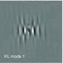
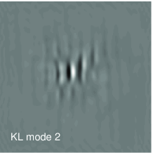
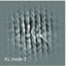
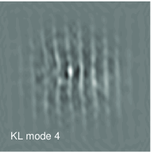
Figure 3: The first four Karhunen-Loeve eigenvectors are shown for a perturbed roll state near the skew-varicose boundary of Rayleigh-Bénard convection. The eigenvectors are ordered by their eigenvalues (largest to smallest), which are propotional to the amount of power contained in the corresponding eigenvector.

The spatial structures of the first four KL vectors are shown in Fig. 3. We find that the first 24 basis vectors capture over 90% of the total power, so an embedding space spanned by these vectors represents well the relaxational dynamics about the straight roll pattern. In our convection experiments, the KL eigenvectors show two distinct length scales. The first two dominant vectors are spatially localized, while the remaining vectors are spatially extended. This is consistent with earlier work as suggested in egolf1 .

More quantitative information can be obtained by finding the eigenmodes of the system, excited by the perturbation, and their growth rates. These can be extracted from a nonlinear least squares fit with the cost function

$$E_{n}=\sum_{i,s,t}\left[{\bf x}^{s}_{i}(t)-\left({\bf x}^{s}_{i}(\infty)+\sum_{k=1}^{n}A^{s}_{k}{\bf m}^{k}_{i}e^{\lambda_{k}t}\right)\right]^{2},$$ (2)

where ${\bf x}^{s}_{i}(t)$ is a projection of the perturbation at time $t$ in the time series $s$ onto the $i$th KL basis vector. In the fit ${\bf m}^{k}$ and $\lambda_{k}$ are the $k$th eigenmode and its growth rate and $A^{s}_{k}$ is the initial amplitude of the $k$th eigenmode excited in the experimental time series $s$. The fixed points ${\bf x}^{s}(\infty)$ are chosen to be different for the differing time series in the ensemble to account for a slow drift in the parameters and we assume that only $n$ eigenmodes are excited.

The results for an ensemble of time series corresponding to seven point perturbations applied across a wavelength of the pattern with $n=6$ are shown in Figs. 4-5. (With seven different initial conditions we cannot hope to distinguish more than seven different modes). In particular, Fig. 4 shows the projection of the experimental time series and the least squares fit on the plane spanned by the first two KL basis vectors. Such extraction of the linear manifold in experiments on spatially extended systems without the knowledge of the dynamical equations of the system aids in the application of techniques that are well developed for low dimensional systems. The manifolds of fixed points and periodic orbits are of particular interest in chaotic systems.

Figure 4: A two-dimensional projection of the experimental time series (symbols) and the least squares fits (continuous curves). The time series have been shifted such that the fixed point is at the origin.

The extracted growth rates $\lambda_{k}$ are shown in Fig. 5. Not surprisingly, since the pattern is stable the growth rates are negative. The leading eigenmode (see Fig. 6) is spatially extended and shows a diagonal structure characteristic of the skew-varicose instability in an unbounded system. This is also expected as the pattern is near the skew-varicose instability boundary. The second eigenmode is spatially localized and has no analog in spatially unbounded systems. The subsequent modes are again spatially delocalized and likely correspond to the Goldstone modes of the unbounded system (e.g., overall translation of the pattern) which are made weakly stable due to confinement by the lateral boundaries of the convection cell.

If the system is brought across the stability boundary, one of the modes is expected to become unstable (without significant change in its spatial structure), thereby determining further (nonlinear) evolution of the system towards a state with a pair of dislocation defects. We would also expect the spatially localized eigenmodes (like the second one in Fig. 6) to preserve their structure if the base state is smoothly distorted (as it would be, e.g., in the SDC state shown in Fig. 1), indicating the same type of a spatially localized instability. Our further experimental studies will aim to confirm these expectations.

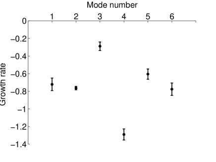
Figure 5: The growth rates of the six dominant eigenmodes and the error bars extracted from the least squares fit. The growth rates have been non-dimensionalized by the vertical thermal diffusion time.

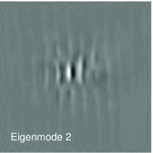
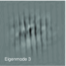
Figure 6: Four dominant eigenmodes extracted from the least squares fit.

Defects represent a type of “coherent structure” in spiral defect chaos. Previous efforts have used coherent structures to characterize spatiotemporally chaotic extended systems in both models sirovich and experiments wolf ; the use of coherent structures to parametrize the invariant manifold was pioneered by Holmes et al. holmes in the context of turbulence. In practice coherent structures are usually extracted using the Karhunen-Loéve (or proper orthogonal) decomposition of time series of system states, which picks out the statistically important patterns. This prior work has met with only limited success – indeed, it is unclear whether statistically important patterns are dynamically important. An alternative approach has been proposed by Christiansen et al. christiansen , who suggested instead to use the recurrent patterns corresponding to the low-period unstable periodic orbits (UPO) of the system, which are dynamically more important. Our work sets the stage for attempting the more ambitious task of extraction of UPOs and their stability properties from experimental data.

Summing up, we have developed an experimental technique which allows extraction of quantitative information describing the dynamics and stability of a pattern forming system near a fixed point. This technique should be applicable to a broad class of patterns, including unstable fixed points, periodic orbits and segments of chaotic trajectories. Moreover, we expect that a similar approach could be applied to other pattern forming systems, convective or otherwise, as long as a method of spatially distibuted actuation of their state can be devised.

References

- (1) M. C. Cross and P. C. Hohenberg, Rev. Mod. Phys. 65, 851-1112 (1993)
- (2) P. Manneville, Dissipative structures and weak turbulence (Academic Press, 1993).
- (3) S. W. Morris, E. Bodenschatz, D. S. Cannel and G. Ahlers, Phys. Rev. Lett. 71, 2026-2029 (1993)
- (4) D. A. Egolf, E. V. Melnikov and E. Bodenschatz, Phys. Rev. Lett. 80, 3228-3231 (1998).
- (5) D. A. Egolf, I. V. Melnikov, W. Pesch and R. E. Ecke, Nature 404, 733-736 (2000)
- (6) P. J. Holmes, J. L. Lumley, and G. Berkooz, Turbulence, coherent structures, dynamical systems and symmetry (Cambridge University Press, 1996).
- (7) L. Sirovich, Physica A 37, 126 (1989)
- (8) F. Qin, E. E. Wolf and H. C. Chang, Phys. Rev. Lett. 72(10), 1459 (1994)
- (9) F. Christiansen, P. Cvitanovic and V. Putkaradze, Nonlinearity 10, 55-70 (1997).
- (10) F. H. Busse, J. Math. Phys. 46, 140 (1967)
- (11) M. M. Chen and J. A. Whitehead, J. Fluid Mech. 31, 1 (1968); F. H. Busse and J. A. Whitehead, J. Fluid Mech. 47, 305 (1971).
- (12) D. Semwogerere and M. F. Schatz, Phys. Rev. Lett. 88, 054501(2002)