Correlation amplitude and entanglement entropy in random spin chains
Abstract
Using strong-disorder renormalization group, numerical exact diagonalization, and quantum Monte Carlo methods, we revisit the random antiferromagnetic XXZ spin-1/2 chain focusing on the long-length and ground-state behavior of the average time-independent spin-spin correlation function . In addition to the well-known universal (disorder-independent) power-law exponent , we find interesting universal features displayed by the prefactor , if is odd, and , otherwise. Although and are nonuniversal (disorder dependent) and distinct in magnitude, the combination is universal if is computed along the symmetric (longitudinal) axis. The origin of the nonuniversalities of the prefactors is discussed in the renormalization-group framework where a solvable toy model is considered. Moreover, we relate the average correlation function with the average entanglement entropy, whose amplitude has been recently shown to be universal. The nonuniversalities of the prefactors are shown to contribute only to surface terms of the entropy. Finally, we discuss the experimental relevance of our results by computing the structure factor whose scaling properties, interestingly, depend on the correlation prefactors.
pacs:
75.10.Pq, 75.10.Nr, 05.70.JkI Introduction
Random low-dimensional quantum spin systems have been intensively investigated recently. The interplay between disorder, quantum fluctuations, and correlations generates low-temperature phase diagrams with exotic phases. igloi-review In this context, one of the most investigated systems is the random antiferromagnetic (AF) quantum XXZ spin- chain, whose Hamiltonian reads
| (1) |
in which labels the chain sites, are the usual spin- operators, ’s are positive uncorrelated random variables drawn from a probability distribution , and ’s are anisotropy parameters, also random uncorrelated variables.
The clean system, and , is a Tomonaga-Luttinger liquid for , with well-known asymptotic ground-state correlation functions, luther-peschel-xxz ; haldane-conjecture
| (2) | ||||
| (3) |
as . The clean-system exponent is luther-peschel-xxz . At the “free-fermion” point , the prefactors of the leading terms are known exactly, lieb-schultz-mattis ; mccoy-68 being given by and . foot-mccoy Away from this point (), analytical forms for and were derived by Lukyanov and Zamolodchikov lukyanov-zamolodchikov-97 ; lukyanov-prefactor and checked numerically later on. hikihara-furusaki-98 Furthermore, the constant , evaluated numerically in Ref. hikihara-furusaki-98, , is at least 1 order of magnitude smaller than . At the isotropic point , irrelevant operators become marginal, yielding logarithmic corrections affleck-prefactor ; lukyanov-npb-98
| (4) |
For , a spin gap opens and the system enters an antiferromagnetic Ising phase; otherwise, for , the chain becomes a gapped Ising ferromagnet.
Disorder strongly modifies the behavior in the clean critical regime. It was shown that even the least amount of disorder in destabilizes the Tomonaga-Luttinger phase, provided . doty-fisher For , a finite amount of disorder is required to destabilize the clean phase. The low-energy behavior of the random AF spin- chain then corresponds to a random-singlet phase, characterized by activated dynamical scaling with a universal “tunneling” exponent , i.e., length () and energy () scales are related through , irrespective of . fisher94-xxz Moreover, the transverse and the longitudinal mean spin-spin correlation functions decay as a power law for large distances, both with the same universal exponent . doty-fisher ; fisher94-xxz The mean value of the correlation function is dominated by rare widely separated spin pairs coupled in strongly-correlated singlet states. The remarkable fact that all correlations (, and ) decay with the same exponent, irrespective of , can be ascribed to the isotropy of the singlet state. In contrast, the typical value of the correlation function decays as a stretched exponential . These results were obtained by using the most successful theoretical tool to investigate such systems, the real-space strong-disorder renormalization-group (SDRG) method, first introduced in Refs. MDH-PRL, and MDH-PRB, .
The main idea behind the SDRG method is to gradually lower the energy scale by successively coupling the most strongly interacting spin pairs into singlet states. At each step of the renormalization transformation, one such pair is decimated out of the chain, and its remaining neighboring spins become connected by a weaker renormalized coupling constant, calculated within perturbation theory. Thus, in this framework, the ground state can be viewed as a collection of “noninteracting” singlets formed by arbitrarily distant spin pairs. Although this description is not strictly exact, spin pairs do couple in states arbitrarily close to singlets. hoyos-rigolin
Recently, efforts to compute certain numerical prefactors on disordered systems have been made. Fisher and Young fisher-young-RTFIM have shown that the end-to-end correlation amplitude of the random transverse-field Ising chain at criticality is nonuniversal because of some high-energy small-scale features that are not treated correctly by the SDRG method. It is reasonable to expect that the same holds for bulk correlations. Indeed, no sign of universality was found in the correlation amplitude of the random XXZ chain. henelius-girvin ; laflorencie-correlacao-PRL ; laflorencie-correlacao-PRB
Refael and Moore, refael-moore on the other hand, have considered the mean entanglement entropy (for a recent review, see Ref. review-amico-07, ) between two complementary subsystems (of size ) and . Similarly to the clean system, holzhey-larsen-wilczek ; vidal-etal-prl03 ; calabrese-cardy-jstatmech04 they have shown that , diverging logarithmically with the subsystem size. More interestingly, the prefactor is universal for a large class of systems governed by an infinite-randomness fixed point, namely, the random transverse-field Ising chain at the critical point and the spin-1/2 random antiferromagnetic XXZ chain. Later, this amplitude was shown to be universal for a broader class of systems governed by infinite-randomness fixed points: the random -state Potts chain and the clock chain santachiara-06 and the random antiferromagnetic spin- chain at the random-singlet phase. saguia-entanglement-07 ; refael-moore-07 Moreover, it has also been shown that this amplitude is also universal in a large class of aperiodic chains. juhasz-zimboras ; igloi-juhasz-zimboras-epl07 In the renormalization-group sense, and following Fisher and Young, fisher-young-RTFIM Refael and Moore refael-moore argued that the nonuniversalities of the correlation amplitudes are related to inaccuracies of order of the lattice spacing in the location of the effective spins. Such errors can only contribute a surface term to the entanglement entropy, and therefore, its prefactor should remain universal. Notably, this should explain why all those other models displaying a random-singlet-like ground state show universal entropy prefactors.
Our aim in this work is to further explore the issue of universality in the behavior of ground-state correlation functions in random antiferromagnetic XXZ chains and make some direct links between spin correlations, structure factor, and entanglement entropy. We first calculate exactly, within the SDRG framework, the numerical prefactor of the mean correlation function in the limit , by relating it to the distribution of singlet-pair bond lengths in the ground state. Surprisingly, it turns out to be universal and equals , if is odd, and , otherwise, because the “noninteracting” singlets can only be formed between spins separated by an odd number of lattice sites. Naturally, this result is an artifact of the (perturbative) SDRG scheme, as shown by exact diagonalization (ED) studies of the XX model henelius-girvin ; laflorencie-correlacao-PRL (in which , ) and quantum Monte Carlo (QMC) calculations applied to the isotropic Heisenberg model laflorencie-correlacao-PRB (in which , ). Nevertheless, as we show from ED calculations, in the XX limit, the long-distance behavior of the longitudinal mean correlation function is shown to be very well described by this renormalization-group prediction, while the transverse mean correlation function exhibits two distinct prefactors, and for odd and even , respectively [see Eq. (30)].
Furthermore, we explicitly show that the mean entanglement entropy is directly related to the bond-length distribution of the singlet pairs and, therefore, directly related to the correlation function. This is interesting because it links a pairwise quantity (correlation) with a blockwise one (entropy).
Since such a relation arises in the scenario of “noninteracting” spin singlets, in which nonuniversal effects are omitted, we introduce a toy model in which the correlations between different singlet pairs can be treated exactly. From the toy model, we gain some insight into the microscopic nature of the random-singlet phase and quantify the role of the interactions between the singlets.
The picture emerging from our analytical results, and confirmed by our own ED and QMC calculations, is the following. At long-length scales, the chain can be recast as a collection of noninteracting effective-spin singlets sharing strong pairwise correlations. These effective spins are clusters of original spin variables whose number depends on the details of the coupling constant distribution. With respect to the original spin variables, the singletlike correlations “spread” among the spins in the cluster, an effect which leads to the nonuniversal high-energy contributions discussed in the literature. fisher-young-RTFIM ; refael-moore Here, we go further by quantifying these contributions within the exactly solvable toy model. Interestingly, whenever the correlation is computed along a symmetry () axis, it equals the corresponding -1/4 singlet contribution, i.e., summing the correlations between all pairs of spins sitting at different clusters gives -1/4. For the mean correlation function, the result is that the combination of prefactors is universal. For correlations along a nonsymmetry ( or ) axis, not only the prefactors are nonuniversal but also the combination . This points to the importance of symmetry for the observed universality, a feature which was absent from the previously considered models. fisher-young-RTFIM Finally, effective spins contribute only nonuniversal surface terms to the entanglement entropy, as expected. When one traces completely one of the spin clusters, its contribution to the entanglement entropy is the same as that of a singlet pair; only when the boundary between the subsystems is crossed by one of the clusters does that cluster contribute a nonuniversal term. Therefore, the entanglement-entropy prefactor is universal regardless of the existence of a symmetry axis.
As a supplement, we compute both analytically and numerically the static structure factor , which can be probed by neutron scattering experiments. Interestingly, we show that is dictated by disorder in the small- limit, namely, . This is a consequence of two facts: (i) the decay exponent being universal, and (ii) the magnitude of the numerical prefactors and being different. Moreover, we find that , which implies that is universal for computed along a symmetry axis. On the other hand, the behavior near the AF peak is dominated by the characteristic divergence of the clean system. However, the true divergence at is suppressed by disorder and the peak width is broadened. Since there is no divergence in the case of along the axis in the XX model, disorder universally determines its behavior near the AF peak, i.e., for . Only for is the clean-system behavior found.
The remainder of this paper is as follows. We derive the universal SDRG expression for the mean correlation function in Sec. II, reporting our numerical analyses in Sec. III. Section IV discusses an exactly solvable model that yields instructive results on the origin of the universal behavior of correlation functions. In Sec. V, we derive the entanglement entropy and relate it to the distribution of singlet lengths and to the correlation function. We discuss the experimental relevance of our results by computing the structure factor in Sec. VI. Finally, we make some concluding remarks in Sec. VII.
II Mean correlation function in the strong-disorder renormalization-group framework
We start this section with a brief review of the SDRG method, followed by the derivation of the mean correlation function.
II.1 Strong-disorder renormalization-group method: A brief review
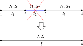
The main idea behind the SDRG method is to reduce the energy scale by integrating out the strongest couplings and renormalizing the remaining ones. In the present case, one locates the strongest coupling constant , say, , and then exactly treats the two-spin Hamiltonian , considering as a perturbation. MDH-PRL At low energies, spins and “freeze” into a (nonmagnetic) singlet state, with the result that they can be effectively removed from the chain, provided that the neighboring spins and are now connected by a renormalized coupling constant
| (5) |
calculated within second-order perturbation theory. The anisotropy parameter is also renormalized to . Note that is smaller than either , , or , leading to an overall decrease in the energy scale. After the decimation procedure, the distance between and , which are now nearest neighbors, is renormalized to
| (6) |
with defined as the distance between the spin and its nearest neighbor to the right. The SDRG decimation scheme is illustrated in Fig. 1.
Clearly, as the SDRG scheme is iterated and the energy scale is reduced, the distribution of effective coupling constants is modified. Searching for fixed-point coupling-constant distributions , Fisher found that there is only one regular stable fixed point
| (7) |
in which is the Heaviside step function and with fisher94-xxz (we set the initial energy scale to 1). This has been named an infinite-randomness fixed point (IRFP) since, as , the distribution becomes infinitely broad, i.e., , where Var and are the variance and mean value of the coupling constants, respectively. Thus, the perturbative decimation procedure becomes more and more precise along the flow because the probability that both and are much smaller than increases as the energy scale is lowered.
A useful quantity to be calculated is the fraction of “active” (not yet decimated) spins at the energy scale . It is obtained from the rate equation
| (8) |
where is the fraction of decimated spins when the energy scale is lowered from to . Hence, close to the fixed point,
| (9) |
Equation (9) directly gives the low-temperature magnetic susceptibility . One iterates the SDRG procedure until the low-temperature scale . Spin pairs decimated at high energy scales are “frozen” into singlet states, and thus their contribution to the magnetic susceptibility can be neglected. As the fixed-point distribution is very broad, all couplings between active spins are very weak compared to , and the active spins can be considered as essentially free spins, each contributing a Curie term to the susceptibility. fisher94-xxz Therefore,
| (10) |
The low-energy modes are also given by Eq. (9). These modes are polarizations of widely separated weakly coupled singlet pairs, decimated at the energy scale for which the mean distance between spins was . Thus, the energy cost to break a singlet of length is
| (11) |
in which . fisher94-xxz This unusual exponential relation between and is named “activated” dynamical scaling and has been dubbed the “tunneling exponent.”
The scaling behavior of the mean correlation function is cleverly obtained when one realizes that typically two very distant spins are not in a singlet state and thus are only weakly correlated. On the other hand, some rare and arbitrarily separated spin pairs that were decimated together are strongly correlated and hence dominate the long-distance behavior of . Therefore, the mean correlation function must be proportional to the total number of spin singlets decimated at the length scale . Since the probability of decimating a spin pair is proportional to the probability that both spins have not been decimated yet, it follows that
| (12) |
with . fisher94-xxz
In contrast, the typical correlation function behaves quite differently. Its long-distance behavior is obtained by the following argument. Suppose spins and are those to be decimated at a given SDRG step, as in Fig. 1. In that case, the correlation between and equals , while the correlation between and is of order . Thus, the typical value of the correlation function will be proportional to the typical value of . Using the fixed-point distribution (7), one finds , i.e., the typical correlation function decays as a stretched exponential, with a nonuniversal prefactor of order unity. fisher94-xxz
II.2 Mean correlation function
We now derive the mean correlation function in a more formal calculation which allows us to compute its amplitude in addition to its power-law decay. In the SDRG framework, the mean correlation function between spins separated by a distance is obtained from the corresponding distribution of singlet-pair bond lengths in the ground state ,
| (13) |
since each singlet contributes a factor of to and there are two spins in each singlet.
The singlet-bond length distribution can be calculated from
| (14) |
where is the probability of finding a coupling constant between and connecting spins separated by a distance between and at the energy scale , and the factor comes from normalization. If we follow exactly the joint probability along the SDRG flow, then we can obtain an exact expression for . In fact, we only need at .
It turns out that we can carry out this task for and couplings taken from the family of initial distributions,
| (15) |
in which gauges the strength of the initial disorder and sets the initial energy scale. foot-igloi We first calculate the density of active spins . For that, we need , which is obtained from the flow equation MDH-PRL
| (16) |
Introducing the Ansatz igloi-det-z-PRL ; igloi-det-z-PRB
| (17) |
into Eq. (16) yields
| (18) |
where . Thus, from the rate equation (8), we obtain
| (19) |
and Eq. (9) is recovered in the low-energy limit .
We now need to follow the SDRG flow of the joint distribution , which is governed by the equation fisher94-xxz
| (20) |
As shown in Appendix A, this can be done exactly by Laplace transforming and using an Ansatz for the corresponding flow equation. The final result for is
| (21) |
where and is the “bare” lattice spacing. Although the leading term of Eq. (21) had been obtained before, fisher94-xxz the explicit dependence on the initial disorder distribution encoded in was not emphasized. As will be shown next, this dependence is essential for our discussion.
Plugging Eqs. (19) and (21) into Eq. (14), we obtain
| (22) | ||||
| (23) |
where
| (24) |
and we used in the last step. As explicitly shown in Eq. (22), the distribution of singlets in the ground state is independent of the initial disorder parameter at all length scales. Moreover, it follows a universal power law in the large-distance limit.
Finally, taking into account that singlets can only be formed between spins separated by distances corresponding to odd multiples of , the mean correlation function takes the universal form
| (25) |
where , irrespective of the initial disorder parameter. Note that Eq. (25) recovers Fisher’s scaling result Eq. (12). In view of the fact that correlations between the spins in a singlet state are isotropic, correlations between components of the spins along a given direction , , or should behave as
| (26) |
with a prefactor given by .
In order to check the prediction of Eq. (25), we calculated the mean correlation function from numerical implementations of the SDRG algorithm on very large chains ( sites), with initial couplings following probability distributions of the form
| (27) |
where , , and . Figure 2 shows, for various chains, the relative difference between the calculated correlation function and the universal prediction, , as a function of . We considered both the XX () and the isotropic Heisenberg () models, for which we averaged over and disorder realizations, respectively. In agreement with the previous analysis, the long-distance behavior of the correlation functions is well described by the universal prediction , regardless of the model under consideration, within an error of less than 5%. Moreover, the mean correlation function of chains DXX, FXX, and HXX (all of which have , as described in the figure caption) are statistically identical at all length scales, in agreement with Eq. (22), which predicts the same short-distance behavior for those spin chains whose coupling constants are distributed according to Eq. (15). Notice that approaches zero for large even for distributions with , which clearly do not belong to the particular class of distributions [Eq. (15)] employed in the derivation of .
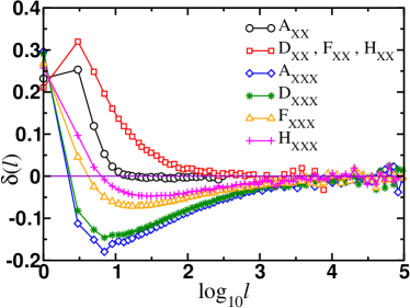
The clear difference between the convergence rates of the mean correlation functions in the XX and Heisenberg models is due to the extra numerical prefactor of present in the recursion relation of the latter model [cf. Eq. (5)], which delays the convergence of to the asymptotic form . This prefactor (which becomes negligible as the SDRG scheme proceeds) alters the relation between length and energy scales, relevant for the derivation of . However, at logarithmically large energy scales, , the simple relation between length and energy scales in Eq. (11) is recovered.
III Numerical results
We now confront the predicted long-distance form of the mean correlation function, given in Sec. II, with numerical results for XX chains, obtained through the mapping to free fermions, and for isotropic Heisenberg chains, obtained by quantum Monte Carlo (QMC) calculations.
III.1 XX chains
We analyzed disordered XX chains with periodic boundary conditions, and coupling constants following box distributions
| (28) |
with , , and , or binary distributions
| (29) |
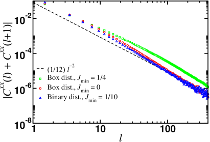
Below, we present results for different choices of parameters. Figure 3 shows the mean longitudinal correlation function as a function of the spin separation for a chain with sites and couplings taken from three probability distributions: two boxlike distributions () with and , and one binary distribution with , in which we average over , , and disorder realizations, respectively. Other disorder distributions give similar results. The short-length behavior approaches the uniform-system result, lieb-schultz-mattis . After a disorder-dependent crossover length, laflorencie-correlacao-PRL ; laflorencie-correlacao-PRB the mean longitudinal correlation function decays as a power law with exponent , and the prefactor clearly approaches the universal value [see Eq. (26)]. Although not shown in the figure, the typical longitudinal correlation function , in contrast, has a nonuniversal prefactor.
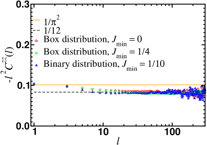
It is remarkable how the random-singlet hallmark appears in Fig. 3. Since both in the clean and in the disordered cases, one could naively think that disorder does not play any role for . However, our statistics are good enough to distinguish the different prefactors. We stress that the fluctuations seen at larger length scales reflect only the increasingly and inevitably poorer statistics, since the number of singlet pairs decreases as and their relative fraction becomes smaller and smaller. Indeed, the mean correlation function is self-averaging. This could be directly double checked from the decrease of the relative fluctuations with the square root of the inverse chain size.
We now turn our attention to the transverse mean correlation function . Compared to its longitudinal counterpart, it behaves quite differently. The short-distance behavior, as in the uniform system, corresponds to a power-law decay with exponent . After a nonuniversal crossover length, the random-singlet behavior is recovered, with a universal exponent , but nonuniversal prefactors, as shown in Fig. 4 and previously pointed out in Refs. henelius-girvin, ; laflorencie-correlacao-PRL, ; laflorencie-correlacao-PRB, . Without loss of generality, the large-distance scaling form of can be written as
| (30) |
with suitably chosen functions and . When couplings are drawn from disorder distributions sufficiently close to the IRFP form of Eq. (7), and are expected to approach the constant values and .
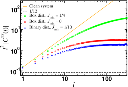
The results from different coupling distributions provide evidence that and indeed approach constant values for arbitrary initial disorder, with and assuming close (but certainly distinct) values. Additionally, it seems that the quantity approaches an asymptotic value close to for sufficiently strong disorder. This can be seen in Fig. 5, where we plot (for odd) the combination . Notice that, for the box distribution with and the binary distribution with , the curves for are reasonably well described by the scaling form in the long-distance limit. However, this is not the case for chains with couplings drawn from the box distribution with , at least up to the sizes studied (, not shown). Indeed, we argue in Sec. IV that deviations from that scaling form should be expected for the transverse correlations in XX chains.
Finally, we report that we have considered also smaller chains ( sites) but with more disordered distributions ( with or ). For the sake of clarity, we have omitted their data in Figs. 3-5. The mean longitudinal correlation function is remarkably well described by the naive SDRG prediction (26). The mean transverse correlation function, on the other hand, is well described by Eq. (30) with .
III.2 XXX chains
We now present QMC results obtained for the SU(2) symmetric model,
| (31) |
with the random AF couplings ’s distributed according to the box distributions
| (32) |
The QMC algorithm we use is based on a stochastic series expansion of the partition function. sandvik91 ; syljuasen-sandvik This is a finite temperature technique which, in principle, allows access to ground-state properties, provided is chosen to be much smaller than the finite-size gap of the system . As already discussed in several works (see, for instance, Refs. laflorencie-correlacao-PRB, and sandvik-perco2D, ; bergekvist-henelius-s1, ; laflorencie-RAF2D, ), the ground-state properties in random spin systems can be very hard to access because extremely small energy correlations might develop between distant spins or spin clusters. For random finite chains, the dynamical exponent is formally infinite since we expect exponentially small couplings to develop at large distances between spins, so that . In order to accelerate the convergence toward the ground state, we used the -doubling scheme sandvik-perco2D and thus performed the QMC measurements at temperatures as small as in units of . We show in Figs. 6 and 7 QMC results for the average spin-spin correlation function in the ground state,
| (33) |
where we perform disorder averaging over independent random samples, as well as space averaging along the periodic chains. Note that the SU(2) symmetry of the Hamiltonian ensures that .
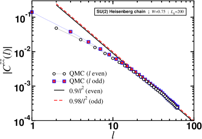
As studied in great detail in Refs. laflorencie-correlacao-PRL, and laflorencie-correlacao-PRB, , there is a crossover phenomenon which is governed by the localization length of the corresponding one-dimensional Jordan-Wigner fermions with random hoppings. In order to be in the asymptotic regime, i.e., in the vicinity of the IRFP, we have to look at system sizes . For the SU(2) symmetric case, has been estimated to be for and for . laflorencie-correlacao-PRB Thus, in order to study the IRFP asymptotic regime, we study two different systems: with sites (see Fig. 6) and with (see Fig. 7). In Fig. 6, we first clearly see the crossover behavior for distances and then the IRFP prediction, Eq. (12), recovered for larger separations. On the other hand, the prediction of Eq. (26) is not verified, and we confirm the observation already made for the XX case. Again, we can write
| (34) |
where and are disorder-dependent prefactors.
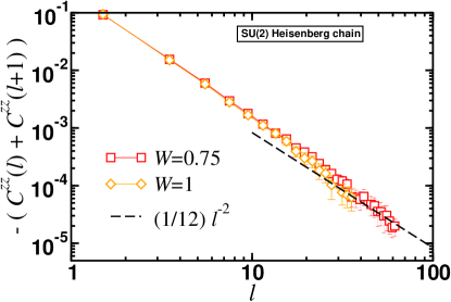
Nevertheless, the universality is recovered when looking at the sum of the prefactors (see Fig. 6) . As shown in Fig. 7, the quantity
| (35) |
seems to behave as for and .
III.3 Discussion
The origin of the apparent universality of is not obvious. It is clear that the breakdown of the SDRG prediction (, ) must be related to the fact that a collection of singlet pairs is not an exact eigenstate of the Hamiltonian for any finite disorder. Although the SDRG method becomes asymptotically exact at low energies, decimations involving spins connected by couplings of the order of the initial energy scale unavoidably lead to significant errors due to the fact that the calculation is perturbative. Thus, instead of singlet pairs, these steps should really involve blocks of three or more neighboring spins, so that correlations “spread” over a few sites (whose number decreases as the strength of the initial disorder increases), forming clusters of correlated spins.
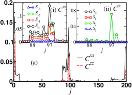
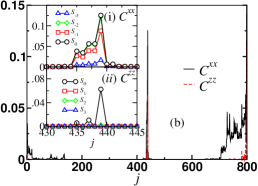
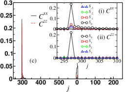
Figure 8 shows the correlation functions and between a reference spin and the -th neighboring spin to the right as a function of for XX chains with couplings drawn from boxlike distributions [panels (a) and (b)] and a power-law distribution [panel (c)]. For the particular realizations in the figure, we find that, decimating the chains according to the SDRG scheme, should couple to in a singlet pair, where , , and for panels (a), (b), and (c), respectively. Indeed, there is a pronounced peak at , as expected from SDRG. In addition, also develops strong correlations with a few spins adjacent to and . As expected for a localized phase, these contributions vanish exponentially at larger distances.
We now can define two spin clusters: The first one is composed by and its neighbors such that the magnitude of the transverse correlation function between and a spin belonging to that cluster is bigger than a certain cutoff, say, , the second cluster is analogous to the first one, but replacing by . Interestingly, the sum of all the longitudinal correlations between the spins in the first cluster and the spins in the second cluster approaches . We thus say that the correlation between and “spreads” among the spins in the clusters, and each of them acts collectively as a single spin, leading to the universal result that at large length scales. However, such feature is not verified when we consider the transverse correlation function. As we show in the next section, this is related to the lack of total spin conservation in the transverse direction.
IV Exactly solvable model
The discussion at the end of Sec. III suggests that the formation of spin clusters is responsible for the failure of the prediction of universal correlation functions, Eq. (25). According to the Marshall-Lieb-Mattis theorem, marshall-prsla-55 ; lieb-mattis the ground state of a spin cluster with antiferromagnetic couplings is a singlet, if the number of spins is even, or a doublet, if the number of spins is odd. Thus, at low enough temperature, a cluster with an even number of spins does not contribute to the magnetic properties of the chain, while a cluster with an odd number of spins can be represented by an effective spin- object.
To gain insight into the origin of the apparent universality of observed in the numerical calculations of Sec. III, we now consider a chain that, at low energies, can be interpreted as being composed of a certain fraction of “effective” spins and a fraction of remaining “original” spins. Each effective spin represents a cluster with an odd number of original spins. For simplicity, we assume here that each effective spin represents a cluster with only three original spins. In addition, we locate the effective spin at the position corresponding to the middle spin of the underlying three-spin cluster. With this restriction, if the effective chain contains spins (original and effective ones), there are, in fact, underlying original spins involved. Moreover, if there are spins between a given spin pair in the effective chain, we say that is the “effective” distance between the spins in that pair. [This is not the same as the renormalized distance defined in Eq. (6).]
Now, we choose the couplings in the effective chain from a probability distribution like that in Eq. (15), with , so that it is sufficiently close to the infinite-disorder fixed-point distribution and the occurrence of “bad” decimations is highly improbable. With this choice of couplings, it follows from Eq. (23) that, in terms of the effective lengths , the effective singlet distribution is given by
| (36) |
for odd , while for even . Therefore, the average number of singlets of effective length in the effective chain is given by
| (37) |
with restricted to odd values.
In order to obtain the ground-state correlations in the underlying chain, we have to determine the distribution of singlet lengths in terms of the underlying original distances , and these will depend on how many effective spins are located between the two spins in a given singlet. Let us consider a singlet formed between spins separated by an effective distance . Hence, there are intermediate spins, of which we assume are effective ones. Note that there are three possible types of singlets (see Fig. 9): a pair of original spins (type ), one original spin and one effective spin (type ), and a pair of effective spins (type ). If the singlet is of type , then the underlying distance is given by ; if the singlet is of type , then ; and for singlets of type , . We immediately conclude that, while singlets of types and are associated with odd underlying distances (since is odd), singlets of type are associated with even underlying distances. This leads to the appearance of correlations between spins separated by even distances, as in our numerical calculations, and in contrast to the assumption of the SDRG approach.
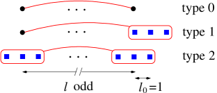
For a singlet of length , the number of intermediate effective spins varies between and . The probability of finding exactly intermediate effective spins is given by
Thus, the numbers of singlets of types , , and with underlying length are given, respectively, by
| (38) |
| (39) |
and
| (40) |
with
| (41) |
In the limit of large , the sum in can be written as an integral, which can be calculated by Laplace’s method, using Stirling’s approximation. The final result is
| (42) |
Consequently,
| (43) |
| (44) |
and
| (45) |
In order to calculate the ground-state correlations , with , let us focus on a fixed odd value of . There are contributions to and coming from singlets of type , with underlying length ; from singlets of type , with lengths and ; and from singlets of type , with lengths , , and . If we denote by () the “weight” of a spin in either end (in the middle) of a three-spin cluster to the component of an effective spin (see Appendix B), we can combine all contributions to write (see Fig. 9)
| (46) |
and
| (47) |
so that, to leading order in , we have
| (48) |
and
| (49) |
Note that the above results are significantly different from the bare SDRG results of Sec. II, most notably in that the average correlation is, in general, not zero for even . Both and decay with the random-singlet exponent , but with different prefactors and , respectively. However, we have
| (50) |
For the XXZ chain, irrespective of the initial anisotropy , the component of the total spin is a good quantum number, assuming the value in the (singlet) ground state. This means that the sum of the ground-state correlations between a given spin and all other spins in the chain is equal to . Since this is also true for an effective spin, it follows that (as can be easily verified explicitly; see Appendix B), and we must have
| (51) |
irrespective of the concentration of effective spins (and thus of the initial disorder). Furthermore, in the Heisenberg limit (), owing to the SU(2) symmetry, we also have
| (52) |
This last result, however, is not valid for . In particular, in the XX limit, for which , we obtain
| (53) |
yielding a weak dependence on .
For the isotropic Heisenberg chain and for , the analytical results derived in this section are in agreement with the numerical results in Sec. III, strengthening the conjecture of a universal behavior for sum of prefactors of the longitudinal ground-state correlations in random XXZ chains. The presence of larger effective-spin clusters (as typically occurs for weaker disorder; see Fig. 8) should not change the conclusions of this section concerning the universality of , since the sum of all the weights of the original spins belonging to an effective cluster is identically 1 when computed with respect to the symmetry axis.
V Entanglement entropy and its relation to the correlation function
In this section, we discuss the relation between the entanglement entropy and the ground-state mean correlation function .
The entanglement entropy between two complementary subsystems and is given by
| (54) |
where is the length of one of the subsystems,
| (55) |
is the reduced density matrix obtained by tracing out the degrees of freedom of subsystem in the ground-state density matrix , and is a set of states spanning the degrees of freedom of (with a similar definition for ).
In the SDRG framework, the ground state of random XXZ chains is a collection of independent singlet pairs, i.e.,
| (56) |
where denotes the -th singlet pair and is the total number of spins in the chain (see Fig. 10).

As the entanglement entropy between two spins in a singlet state is , foot-entropy the total entanglement entropy due to a given choice of subsystems and is equal to times the number of singlet pairs in which one spin belongs to and the other one to (see Fig. 10). Using this fact, Refael and Moore refael-moore calculated the mean number of times that each bond is decimated, which is equivalent to the mean number of singlet lines crossing a given boundary. They found that the mean value of the entanglement entropy grows as , with being a universal number. This is reminiscent of the entanglement entropy in conformally invariant (clean) one-dimensional quantum systems, which increases as , where is the central charge, a signature of the universality class of conformally invariant systems. holzhey-larsen-wilczek ; calabrese-cardy-jstatmech04 In the clean critical XXZ chain, .
We now rederive the mean entanglement entropy by relating it to the distribution of singlet lengths [see Eq. (23)] and thus to the SDRG mean correlation function [see Eq. (25)]. By definition, the mean value of the entanglement entropy between a subsystem of length and the rest of the chain is the sum of the entropies of all subsystems of length , divided by . (In a -site chain with periodic boundary conditions, there are different subsystems with the same length.) The contribution of a given singlet of length depends on the relation between and . If , there are different subsystems of length whose boundaries are crossed by the singlet line [see Fig. 11(a)]. Likewise, different subsystems have their boundaries crossed by a singlet of length [see Fig. 11(b)]. Thus,
| (57) |
where is the number of singlets with length in the ground state and is the contribution of a singlet pair to the entanglement entropy.

As shown in Sec. II, is simply related to the correlation function by . Thus, substituting Eq. (25) into Eq. (57), and noting that for even , we obtain, for and ,
| (58) | ||||
| (59) | ||||
| (60) |
in which , while and are nonuniversal constants that depend on the short-distance details of . In this way, we recover the result obtained by Refael and Moore. Yet another derivation of the above result is presented in Appendix C.
Note that Eq. (58) relates the mean value of the entanglement entropy to the mean correlation function. This relation is valid only in the context of infinite-randomness spin chains, where both quantities are dominated by rare spin singlets. In AF spin-1/2 chains without disorder, for instance, such relation is no longer valid, and the correct expression is far from simple (though an efficient valence-bond approach can be developed to study block entanglement properties alet-etal-07 ).
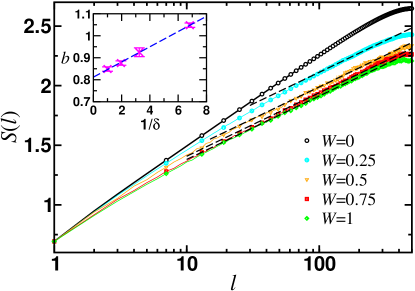
Contrary to the naive universal form [Eq. (26)] of the ground-state correlation function, which is found not to hold when confronted with exact diagonalization or QMC calculations, the universal prediction of Eq. (60) is fully supported by numerical results (see Ref. laflorencie-entanglement, ) and, as shown in Fig. 12, does not depend on the initial disorder strength. In view of the relation between these two quantities, revealed by Eq. (58), the arising question is how these seemingly contradictory results can be reconciled.
We address this question by looking at the entanglement entropy of the exactly solvable model of Sec. IV. The ground state of the model can be viewed as a collection of singlets of three different types (see Fig. 9). So, although Eq. (58) can no longer be used, the entanglement entropy is still related to the distributions of singlet lengths, in analogy with Eq. (57). However, we must remember that an effective spin represents a three-spin cluster. It can be easily shown that the entanglement entropies between a three-spin cluster and a single spin, as well as between two three-spin clusters, are also given by . However, since we have to average over all different possible subsystems of a given size, we must take into account situations in which one of the spins in a three-spin cluster lies in a different subsystem than the other two. When averaged over all subsystems and singlet types, these “internal” contributions, being only boundary effects, lead to an additional constant term and thus do not affect the scaling properties of the entanglement entropy. Explicitly, we have
| (61) |
in which , , and are the average entanglement entropies due to singlets of types , , and , respectively. From Eq. (57), taking into account the “internal” contributions , we can immediately write , for , and , as
| (62) |
with given by Eqs. (43)-(45). Bearing in mind that and are zero for even , while is zero for odd , we can use the fact that
| (63) |
for odd , to conclude from Eq. (61) that
| (64) |
again with , and an -dependent constant , as in Eq. (60).
Although this exactly solvable model yields a nonuniversal ground-state correlation function , the entanglement entropy does follow the universal form derived by Refael and Moore. refael-moore This last result and the numerical confirmation of the universality of (see Ref. laflorencie-entanglement, and Fig. 12) suggest that a description of the ground state of random XXZ chains in terms of a collection of independent singlets remains valid at sufficiently large distances, provided we use the notion of effective spins already discussed in the previous sections.
Finally, we should mention that the notion of the nonuniversality of the correlation amplitude due to high-energy small-scale details was first considered and investigated by Fisher and Young. fisher-young-RTFIM Later, Refael and Moore refael-moore realized that such details only contribute to the inaccuracies in the location of the low-energy effective spins, which lead only to a surface term contribution to the entanglement entropy, as we have formally shown here.
VI Structure factor
In this Section, we compute the static structure factor
| (65) |
which is straightforwardly related to the mean spin-spin time-independent correlation function and is directly measured in neutron scattering experiments. Indeed, neutron scattering experiments probe the dynamical structure factor
| (66) |
which reduces to in Eq. (65) after an integration over .
There are three noteworthy properties of :
| (67) |
| (68) |
where the sum is over the first Brillouin zone, and
| (69) |
where is the total spin along the direction and means its expectation value on the ground state. Hence, for the XX model and for the isotropic case. Note that, in the continuum limit, Eq. (68) leads to .
We now show our numerical results on the static structure factor for the disordered chain in the XX and XXX models. We anticipate that all three properties [Eqs. (67)-(69)] are obeyed by our numerical results.
VI.1 XX model
Figure 13 shows the longitudinal structure factor in the XX model for the clean system [in which (see inset)] and various disordered chains. Because the longitudinal mean correlation function depends very weakly on the disorder (only through the crossover length) and its universal amplitude in the disordered case is very close to the clean-system value ( in comparison to ; see Secs. II.2 and III.1), the longitudinal structure factor is, for all practical purposes, universal.
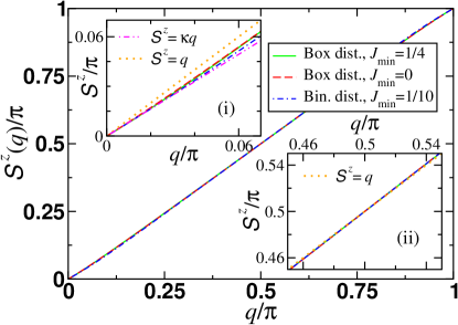
In general, due to spin conservation and the fact that for even , equals and at the points and , respectively. Moreover, it can be shown that has inversion symmetry around the point , i.e., , for , which implies .
Let us now consider the effects of disorder more closely. Because the behavior of for small is dominated by the large- behavior of the longitudinal correlation function, it follows that , where is a universal constant [see inset (i) of Fig. 13]. In the same way, because for even , the behavior near is also dominated by disorder. In this case, . This is verified by the data of Fig. 13, but not shown for clarity. Finally, because the Fourier series [Eq. (65)] at near selects small values of , the behavior near is dominated by the clean-system prediction, as shown in inset (ii) of Fig. 13. Note that all these arguments are valid because for even .
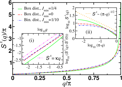
We now discuss the behavior of (see Fig. 14), in which disorder plays a more prominent role. In the absence of disorder, , where is the Luttinger liquid parameter [see Eq. (2)], and and (Ref. mccoy-68, ) are positive constants. Since the first term is monotonic, it dominates the structure factor for . Hence, . The second (staggered) term gives a subdominant contribution . Near the AF peak, ; however, the second term dominates, yielding a divergent contribution, namely, , for .
Quenched disorder dramatically changes the above scenario. Rewriting the transverse correlation function [see Eq. (30)] as (where , if is odd, and , otherwise), it becomes clear that is dominated by the first term: , where + nonuniversal contributions [see inset (i) of Fig. 14]. Note that this result strongly relies on the fact that is nonzero; otherwise, would be dominated by the short length scale contributions to , which follow the clean-system prediction.
The characteristic AF divergence near is suppressed by disorder, as shown in inset (ii) of Fig. 14. For , where is the crossover length above which the correlation function is dominated by the disorder, saturates to a constant approximately equal to . Finally, because Eq. (68) has to be satisfied, the decrease of the AF peak is accompanied by its broadening as disorder increases [see inset (ii) of Fig. 14].
VI.2 XXX Model
We now turn our attention to the isotropic Heisenberg model (see Fig. 15).
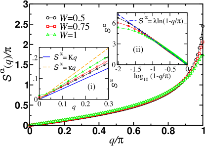
Similarly to the XX model, the universal features of the correlation amplitude yield a universal structure factor for : , since is universal. By coincidence, the clean system prediction also scales linearly, pereira-etal , however, with a different slope which is the Luttinger liquid parameter. As shown in inset (i) of Fig. 15, is linear, but apparently with no universal slope. However, although we have statistical fluctuations and finite-size effects, a close inspection of our data for shows that fits better than .
The logarithmic divergence at the point is suppressed by disorder. As shown in inset (ii) of Fig. 15, follows the clean-system divergence up to a crossover vector , where is the crossover length above which the correlation exponent follows the long-distance prediction of the disordered system. Beyond , saturates at a non-universal constant proportional to . We note that the clean-system prediction depicted by the dashed line, , is actually the prediction of the Haldane-Shastry model, haldane-r-2-spinchain ; shastry-longrange-spinchain which is a good approximation to the Heisenberg model for . karbach-94 ; karbach-97 For , diverges as , consistent with for .
VI.3 Discussion
Summarizing, is peaked at , , in both models, while it approaches zero at , reflecting the antiferromagnetic quasi-long-range order. Near , the low-energy behavior of the structure factor is dominated by the short-length scale behavior of the spin-spin correlation function, and thus its scaling is determined by the physics of the clean system. However, the true divergence is completely suppressed by disorder, and the peak becomes shorter and broader. On the other hand, the structure factor vanishes universally for [for in the XX model, one may consider the quantity ] as a consequence of two features: (i) the power-law scaling of the mean spin-spin correlation function , with universal exponent doty-fisher ; fisher94-xxz and (ii) the amplitudes and being different in magnitude. Moreover, due to the universal features of these amplitudes, vanishes as , with a universal , if is a symmetry axis, and a nonuniversal , otherwise.
We now briefly discuss a controversy that has appeared in the literature. The dynamical structure factor was theoretically studied in Refs. huse-structurefactor-PRL, and huse-structurefactor-PRB, within the SDRG framework (and thus, in the small- limit) and experimentally studied in Refs. masuda, ; masuda-erratum, ; zheludev, , mainly by measuring the local dynamical structure factor [obtained when one integrates over ] for the compound BaCu2(Si0.5Ge0.5)2O7. Previously, it had been thought that this compound is a good experimental realization of the random AF spin-1/2 chain with quenched bond randomness, since both the experimentally determined static magnetic susceptibility and local dynamical structure factor were found to be in good agreement with the strong-disorder theoretical predictions. masuda However, further and more precise measurements appeared to be in contradiction with the strong-disorder theoretical scaling of . masuda-erratum ; zheludev Interestingly, the magnetic susceptibility measurements remained in agreement with the theoretical prediction for the disordered system. masuda-erratum This led to a puzzle. Thermodynamical quantities seem to be dominated by the physics of the disordered system, whereas spin correlations seem to show the clean system physics.
We tentatively argue that the low-energy behavior of the quantity investigated experimentally may not be dominated by the physics of the disordered system, even if the system itself is governed by a strongly disordered fixed point. The quantity is obtained from an integration over all values of . Therefore, it is dominated by the antiferromagnetic peak . Such large momentum reflects the shortest length scales of the time-dependent correlation function, whose behavior is expected to be dominated by the physics of the disorder-free system, as in the case of the time-independent correlation function. Hence, the experimental determination of the full -dependent would be highly desirable.
Recently, it was shown mucio-07 that the spin-1/2 compound MgTiOBO3 displays a remarkable random-singlet signature for the magnetic susceptibility in a wide and accessible range of temperature. It would be interesting to perform neutron scattering experiments on this compound in order to check the predictions shown here for the static structure factor.
VII Conclusions
In this paper, we revisited the ground-state properties of random-bond antiferromagnetic quantum spin- chains using analytical and numerical tools. We focused on the question of the universality of the spin-spin correlation function and of the average entanglement entropy , as functions of the distance , as well as the connection between them.
By following exactly the SDRG flow of a family of coupling-constant distributions, we showed that the SDRG approach predicts a fully universal power-law scaling form of the pair correlation function , in which both the prefactor and the decay exponent are disorder independent. However, the SDRG prediction is strictly valid only in the limit of infinite randomness. Exact diagonalization and quantum Monte Carlo calculations on finite chains showed that this purported universality does not hold, except for the correlations along the symmetry axis in the XX model. Moreover, these numerical results reveal different correlation amplitudes for spins separated by odd and even distances, and , respectively. Nevertheless, we showed numerical evidence that the combination , at least for the XXX model and for correlations along the symmetry axis in the XX model, is indeed universal and agrees with the SDRG prediction if we consider that spin clusters themselves develop singletlike correlations. In other words, the correlations of random singlets spread among spins in the clusters.
As the average number of spins in a cluster depends on the details of the coupling-constant distribution, correlation-function prefactors are nonuniversal. However, the conservation law for the total spin component along the symmetry axis guarantees that correlations “spread” over all spins in the effective-spin singlets, leading to the universality of . This hypothesis was confirmed analytically in an exactly solvable model, in which a number of three-spin clusters were introduced into an infinite-disorder random-bond chain. Interestingly, the fact that and are different in magnitude has important experimental relevance: the small- behavior of the structure factor is dominated by disorder. We have argued that -resolved neutron scattering experiments may be able to probe the universal features of those amplitudes.
We also rederived the average ground-state entanglement entropy , relating it to the mean correlation function. In contrast to the nonuniversality of when considering along a nonsymmetry axis, the universal form of first derived by Refael and Moore refael-moore was shown to hold for the exactly solvable model with effective spins, in agreement with the numerical data presented in Sec. V and previously elsewhere. laflorencie-entanglement
Note added. Recently, we became aware of Ref. xu-ying-wan, where the dynamical structure factor is also studied and the controversy mentioned at the end of Sec. VI is considered.
Acknowledgements.
J.A.H. would like to thank R. G. Pereira, T. Vojta, and D. A. Huse for useful discussions. J.A.H. and N.L. are grateful for the hospitality of the Pacific Institute for Theoretical Physics and Les Houches Summer School where part of this work was performed. This work was partially supported by Fapesp under Grant No. 03/00777-3, by NSF under Grant No. DMR-0339147, by Research Corporation (J.A.H.), by CNPq/FUNCAP under Grant No. 350145/2005-9 (A.P.V.), by NSERC, by the Swiss National Fund, by MaNEP (N.L.), and by CNPq under Grant No. 305971/2004-2 (E.M.). Part of the simulations have been preformed using the WestGrid network.Appendix A Calculation of
Laplace transforming Eq. (20) with respect to the length variable yields
| (70) |
where . We now substitute the Ansatz igloi-det-z-PRL ; igloi-det-z-PRB
| (71) |
into Eq. (70) and find a pair of equations,
| (72) | |||||
| (73) |
with the boundary conditions . Since
| (74) |
we find the solutionsigloi-det-z-PRB
| (75) | |||||
| (76) |
where is a constant of the flow, defined by . Moreover, is a real number since , which can be shown by considering an explicit calculation of the mean distance between the “active” spins,
| (77) | |||||
As , Eq. (77) ensures that .
The boundary conditions lead to , and so . From
| (78) | |||||
one finds , the last step coming from the definition , where is the initial mean distance between the sites. For simplicity, we consider that initially all spins are uniformly separated, i.e., is the lattice spacing. The constant thus equals and depends on the two parameters of the problem, the initial length parameter and the initial disorder parameter . This is a consequence of the fact that the magnitude of a coupling constant shared by two spins a distance apart is correlated with , and thus the joint distribution cannot be written as .
Appendix B Renormalization of a three-spin cluster
A cluster of three spins , , and , connected by antiferromagnetic XXZ couplings, can be replaced at low energies by an effective spin-1/2 object. If the three-spin Hamiltonian is given by
| (82) | |||||
with and , then the ground state is doubly degenerate. Thus, we can define an effective spin such that, in the doublet subspace, the original spins are represented by “weights” defined by vieira-aperiodic-PRB
| (83) |
with and
| (84) |
| (85) |
| (86) |
| (87) |
Appendix C Another derivation of the entanglement entropy in the strong-disorder renormalization-group framework
Following Refael and Moore, refael-moore we exactly calculate the mean number of times a given bond is decimated, which corresponds to the mean number of singlet links crossing a given point in the chain at the energy scale . Averaging over all the sites in the lattice, this is simply the sum of the lengths of all bonds decimated until the energy scale , divided by the chain length:
| (88) |
Using the results in Eqs. (19) and (21) we find that
| (89) | |||||
| (90) |
where we have used the relation between length and energy scales in Eq. (78). Again, the reader should be aware of an extra 1/2 prefactor when integrating over , due to the fact that singlet lengths are restricted to odd multiples of . Finally, because any subsystem has two boundaries,
| (91) |
in which is a universal constant. Note that the constant presented here has no physical meaning. Although its value does not depend on the initial disorder strength in this derivation, deviations from such value are expected due to the spin clusters crossing the boundaries (see Sec. V).
References
- (1) F. Iglói and C. Monthus, Phys. Rep. 412, 277 (2005).
- (2) A. Luther and I. Peschel, Phys. Rev. B 12, 3908 (1975).
- (3) F. D. M. Haldane, Phys. Rev. Lett. 45, 1358 (1980).
- (4) E. Lieb, T. Schultz, and D. Mattis, Ann. Phys. 16, 407 (1961).
- (5) B. M. McCoy, Phys. Rev. 173, 531 (1968).
- (6) There is an extra factor of 4 in Eq. (6.9) of Ref. mccoy-68, .
- (7) S. Lukyanov and A. Zamolodchikov, Nucl. Phys. B 493, 571 (1997).
- (8) S. Lukyanov, Phys. Rev. B 59, 11163 (1999).
- (9) T. Hikihara and A. Furusaki, Phys. Rev. B 58, R583 (1998).
- (10) I. Affleck, J. Phys. A 31, 4573 (1998).
- (11) S. Lukyanov, Nucl. Phy. B 522, 533 (1998).
- (12) C. A. Doty and D. S. Fisher, Phys. Rev. B 45, 2167 (1992).
- (13) D. S. Fisher, Phys. Rev. B 50, 3799 (1994).
- (14) S.-k. Ma, C. Dasgupta, and C.-k. Hu, Phys. Rev. Lett. 43, 1434 (1979).
- (15) C. Dasgupta and S.-k. Ma, Phys. Rev. B 22, 1305 (1980).
- (16) J. A. Hoyos and G. Rigolin, Phys. Rev. A 74, 062324 (2006).
- (17) D. S. Fisher and A. P. Young, Phys. Rev. B 58, 9131 (1998).
- (18) P. Henelius and S. M. Girvin, Phys. Rev. B 57, 11457 (1998).
- (19) N. Laflorencie and H. Rieger, Phys. Rev. Lett. 91, 229701 (2003).
- (20) N. Laflorencie, H. Rieger, A. W. Sandvik, and P. Henelius, Phys. Rev. B 70, 054430 (2004).
- (21) G. Refael and J. E. Moore, Phys. Rev. Lett. 93, 260602 (2004).
- (22) L. Amico, R. Fazio, A. Osterloh, and V. Vedral (2007), arXiv:quant-ph/0703044v1.
- (23) C. Holzhey, F. Larsen, and F. Wilczek, Nucl. Phys. B 424, 443 (1994).
- (24) G. Vidal, J. I. Latorre, E. Rico, and A. Kitaev, Phys. Rev. Lett. 90, 227902 (2003).
- (25) P. Calabrese and J. Cardy, J. Stat. Mech. p. P06002 (2004).
- (26) R. Santachiara, J. Stat. Mech. p. L06002 (2006).
- (27) A. Saguia, M. S. Sarandy, B. Boechat, and M. A. Continentino, Phys. Rev. A 75, 052329 (2007).
- (28) G. Refael and J. E. Moore (2007), Phys. Rev. B 76, 024419 (2007).
- (29) R. Juhász and Z. Zimborás, J. Stat. Mech. p. P04004 (2007).
- (30) F. Iglói, R. Juhász, and Z. Zimborás, Europhys. Lett. 79, 37001 (2007).
- (31) Note that in this case the recursive SDRG procedure is equivalent to that of the critical point of the random Ising chain in a transverse field, for which the coupling-constant distribution flow was exactly obtained before by Iglói and coworkers. igloi-det-z-PRL ; igloi-det-z-PRB
- (32) F. Iglói, R. Juhász, and P. Lajkó, Phys. Rev. Lett. 86, 1343 (2001).
- (33) F. Iglói, Phys. Rev. B 65, 064416 (2002).
- (34) A. W. Sandvik and J. Kurkijärvi, Phys. Rev. B 43, 5950 (1991).
- (35) O. F. Syljuåsen and A. W. Sandvik, Phys. Rev. E 66, 046701 (2002).
- (36) A. W. Sandvik, Phys. Rev. B 66, 024418 (2002).
- (37) S. Bergkvist, P. Henelius, A. Rosengren, Phys. Rev. B 66, 134407 (2002).
- (38) N. Laflorencie, S. Wessel, A. Läuchli, and H. Rieger, Phys. Rev. B 73, 060403(R) (2006).
- (39) W. Marshall, Proc. R. Soc. London. Ser. A 232, 48 (1955).
- (40) E. Lieb and D. Mattis, J. Math. Phys. 3, 749 (1962).
- (41) Notice we are using the logarithm in the natural basis in Eq. (54).
- (42) F. Alet, S. Capponi, N. Laflorencie, and M. Mambrini, Phys. Rev. Lett. 99, 117204 (2007).
- (43) N. Laflorencie, Phys. Rev. B 72, 140408(R) (2005).
- (44) R. G. Pereira, J. Sirker, J.-S. Caux, R. Hagemans, J. M. Maillet, S. R. White, and I. Affleck, J. Stat. Mech.: Theory Exp. 2007, P08022.
- (45) F. D. M. Haldane, Phys. Rev. Lett. 60, 635 (1988).
- (46) B. S. Shastry, Phys. Rev. Lett. 60, 639 (1988).
- (47) M. Karbach, K.-H. Mütter, and M. Schmidt, Phys. Rev. B 50, 9281 (1994).
- (48) M. Karbach, G. Müller, A. H. Bougourzi, A. Fledderjohann, and K.-H. Mütter, Phys. Rev. B 55, 12510 (1997).
- (49) K. Damle, O. Motrunich, and D. A. Huse, Phys. Rev. Lett. 84, 3434 (2000).
- (50) O. Motrunich, K. Damle, and D. A. Huse, Phys. Rev. B 63, 134424 (2001).
- (51) T. Masuda, A. Zheludev, K. Uchinokura, J.-H. Chung, and S. Park, Phys. Rev. Lett. 93, 077206 (2004).
- (52) T. Masuda, A. Zheludev, K. Uchinokura, J.-H. Chung, and S. Park, Phys. Rev. Lett. 96, 169908(E) (2006).
- (53) A. Zheludev, T. Masuda, G. Dhalenne, A. Revcolevschi, C. Frost, and T. Perring, Phys. Rev. B 75, 054409 (2007).
- (54) T. G. Rappoport, L. Ghivelder, J. C. Fernandes, R. B. Guimarães, and M. A. Continentino, Phys. Rev. B 75, 054422 (2007).
- (55) Z. Xu, H. Ying, and X. Wan (2007), arXiv:cond-mat/0703772v1 [cond-mat.str-el].
- (56) A. P. Vieira, Phys. Rev. B 71, 134408 (2005).