Spin accumulation from the non-Abelian Aharonov-Bohm effect

Abstract

Recently, it has been shown that the spin-orbit coupling (SOC) of the Dresselhaus type in $[110]$ quantum wells can be mathematically removed by a non-Abelian gauge transformation. In the presence of an additional uniform magnetic field, such a non-Abelian gauge flux leads to a spin accumulation at the edges of the sample, where the relative sign of the spin accumulation between the edges can be tuned by the sign of the Dresselhaus SOC constant. Our prediction can be tested by Kerr measurements within the available experimental sensitivities.

Spin transport in the presence of spin-orbit coupling has attracted great attention in the field of spintronics. The theoretical prediction of the spin Hall effect Murakami et al. (2003); Sinova et al. (2004) in both $p$ and $n$ type doped semiconductors has lead to the experimental observation of spin accumulation at the sample boundaries Kato et al. (2004); Wunderlich et al. (2005). Spin-orbit coupling is the main cause of spin decoherence in solids. However, recently, it has been realized that certain types of spin-orbit coupling, including models with equal Rashba and Dresselhaus SOCs and the model with Dresselhaus SOC in $[110]$ quantum wells, can be mathematically removed by a non-Abelian gauge transformation Bernevig et al. (2006). In these systems, the spin life time is rendered infinite at a magic wave vector, giving rise to the Persistent Spin Helix Bernevig et al. (2006); Weber et al. (2007).

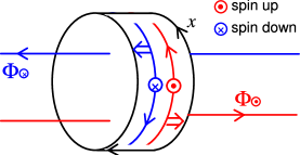
Figure 1: (Color online) Schematic picture of Laughlin-Halperin gauge argument in the Dresselhaus [110] model. The Dresselhaus SOC is equivalent to two pure gauge fluxes, acting oppositely on each spin orientation. The magnetic field points out of the cylindrical surface where the 2DEG lives. Double arrows indicate the direction of the Lorentz force, which leads to the spin accumulation on the edges of the cylinder.

In this letter, we show that the equivalence of the Dresselhaus [110] SOC with a pure non-Abelian gauge flux has another intriguing and observable physical consequence. In the classic understanding of the integer quantum Hall effect, Laughlin and Halperin considered a Gedanken experiment Laughlin (1981); Halperin (1982) in which one adiabatically inserts a pure gauge flux through a cylinder, where the two-dimensional electron gas (2DEG) exists on the cylindrical surface, see Fig. 1. To our knowledge, such a Gedanken proposal has never been realized experimentally. We shall show that the Dresselhaus [110] SOC provides an exact physical realization of this Gedanken experiment, where the gauge flux is opposite for the two different spin orientations. The Dresselhaus SOC $\beta$ can be tuned continuously by changing the thickness of the [110] quantum wells (QWs). By the Faraday’s law of induction, applied separately to both spin orientations, the adiabatic turning of the gauge flux, or equivalently, the Dresselhaus SOC $\beta$, leads to a non-Abelian electric field along $x$ direction Jin et al. (2006), $\mathcal{E}^{x}=2m\partial_{t}\beta(t)\sigma_{z}/\hbar^{2}$. The non-Abelian electric field drives electrons with different out-of-plane spin components to opposite $y$ (Hall) directions, resulting in the spin accumulation at the sample boundaries. Furthermore the relative sign of the spin accumulation between the edges can be tuned by the sign of the SOC constant, and the spin accumulation has a periodic dependence on the SOC constant, with the equivalent Aharonov-Bohm periodicity. This effect can be detected by Kerr measurements within the available experimental sensitivities.

Our starting point is a 2DEG system with Dresselhaus [110] SOC interactions being turned on adiabatically at some initial time, and a small Rashba term which we treat perturbatively. The electrons are confined in the $x$-$y$ plane subjecting to a magnetic field $\vec{B}=B\hat{z},B>0$. There are two intrinsic length scales in our systems, namely the magnetic length $l_{b}=\sqrt{\hbar/eB}$ and the characteristic length of spin-orbit interaction $l_{so}=\hbar^{2}/m\beta$. For a fixed magnetic field the ratio $r=l_{b}/l_{so}$ plays the role of dimensionless SOC constant. We take the periodic boundary condition in $x$ direction and the open boundary condition in the $y$ direction. In the Landau gauge, $\vec{A}=-By\hat{x}$, the single-particle Hamiltonian is given by $H(r)=H_{0}(r)+H_{R}$ with

$$H_{0}=\frac{(\vec{p}+e\vec{A})^{2}}{2m}-\frac{2\beta}{\hbar}(p_{x}+eA_{x})\sigma_{z}+\frac{g_{s}\mu_{B}B}{2}\sigma_{z}+V,$$ (1)

where $\beta$ is the Dresselhaus SOC constant, $-e$, $m$ and $\mu_{B}$ are respectively the charge, effective mass and Bohr magneton of the electron, the lateral confining potential $V(y)$ vanishes for $y\in(-L_{y}/2,L_{y}/2)$, and is infinite otherwise. In the following, we first treat analytically the system $H_{0}(r)$ and then discuss the effect of the Rashba coupling $H_{R}$ perturbatively.

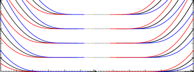
Figure 2: (Color online) $\nu_{n\sigma}$ as a function of $\widetilde{y}_{0}^{(\pm)}=(\pm L_{y}/2-y_{0})/l_{b}$, the orbital center measured from the boundaries in units of $l_{b}$, for positive (‘$+$’) and negative (‘$-$’) edges. The energy spectrum at $r=0$ is shown in black, and those at $r=0.2$ for up and down spin are shown in red and blue.

For the system $H_{0}$ we observe that good quantum numbers are the eigenvalues $p_{x}=\hbar k$ and $\sigma_{z}=\sigma=\pm 1$, therefore $H_{0}$ is diagonalized automatically and we seek solutions of the form $\psi(x,y,r)=\frac{1}{\sqrt{2\pi}}e^{ikx}\phi_{nk}(y,r)$ where $\phi_{nk}$ is a two-component spinor, obeying the one dimensional (1d) Schr$\ddot{\text{o}}$dinger equation

$$\left[-\frac{\hbar^{2}}{2m}\frac{d^{2}}{dy^{2}}+\frac{m\omega_{c}^{2}}{2}(y-y_{0\sigma})^{2}\right]\phi_{nk\sigma}=\varepsilon_{nk\sigma}\phi_{nk\sigma}.$$ (2)

In the above $y_{0\sigma}=y_{0}-2l_{b}\sigma r$ is the orbital center for the spin component $\sigma$ and $y_{0}=l_{b}^{2}k$ is that without SOC. We notice that the $\beta$ term in Eq. (1) corresponds to a pure gauge flux since it can be eliminated by a local non-Abelian gauge transformation $U=\exp{(-i2m\beta x\sigma_{z}/\hbar^{2})}$ with the magnitude of the flux given by $\Phi_{\sigma}=4m\beta L_{x}/\hbar^{2}\propto r$ for $\beta>0$. Therefore, when increasing the flux $\Phi_{\sigma}$ or $r$ adiabatically, the orbital centers of up and down spin components move to the negative and positive Hall directions respectively, leading to accumulations near the opposite edges. The eigenvalues of this system are given by $E_{nk\sigma}=\varepsilon_{nk\sigma}-\hbar\omega_{c}(2r^{2}-g^{\ast}\sigma/4)$ where $\omega_{c}=eB/m$ and $g^{\ast}=g_{s}m/m_{e}$. If we denote the Fermi energy of our system as $E_{F}=\hbar\omega_{c}\nu_{F}$ which depends on the electron density $n_{e}$ and the magnetic field $B=\frac{n_{e}h}{e(\nu_{F}+1/2)}$, the effective Fermi levels for spin-$\sigma$ are then given by $\nu_{F\sigma}=\nu_{F}+2r^{2}-1/2-g^{\ast}\sigma/4$. We assume that the width $L_{y}$ between the two boundaries is large enough so that the two edges are well-separated, then in the bulk region where $|y_{0\sigma}\pm L_{y}/2|\gg l_{b}$, the edge effect can be neglected and $\varepsilon_{nk\sigma}=\hbar\omega_{c}(n+1/2)$ with integers $n$. While in the edge region where $|y_{0\sigma}\pm L_{y}/2|\sim l_{b}$, the confining potential must be taken into account by setting $\phi_{nk\sigma}(y=\mp L_{y}/2,r)=0$. In such a case if we still keep the form $\varepsilon_{nk\sigma}=\hbar\omega_{c}[\nu_{n\sigma}(k)+1/2]$, however, $\nu_{n\sigma}$ is not necessary integers any more, the general solution MacDonald and Středa (1984) to Eq. (2) may be written as

$$\phi_{nk\sigma}(y,r) =e^{-\frac{(y-y_{0\sigma})^{2}}{2l_{b}^{2}}}(CF\left[-\frac{\nu_{n\sigma}}{2};\frac{1}{2};\frac{(y-y_{0\sigma})^{2}}{l_{b}^{2}}\right]$$ (3)

$$+D\frac{y-y_{0\sigma}}{l_{b}}F\left[\frac{1-\nu_{n\sigma}}{2};\frac{3}{2};\frac{(y-y_{0\sigma})^{2}}{l_{b}^{2}}\right])$$

where $F[a;b;z]$ is the confluent hypergeometric function of the first kind. The constants $C$ and $D$ are fixed by requiring $\phi_{nk\sigma}(y\rightarrow\pm\infty)=0$ when considering the negative and positive edges separately, which leads to $\frac{D}{C}=\pm 2\tan\left(\frac{\pi\nu_{n\sigma}}{2}\right)\frac{\Gamma(1+\nu_{n\sigma}/2)}{\Gamma(\frac{1}{2}+\nu_{n\sigma}/2)}$, as well as the normalization of the wavefunction. The discrete eigenvalue spectrum at each given $r$ are then determined by finding the zeros of $\phi_{nk\sigma}(y=\mp L_{y}/2,r)$. The energy spectrum at $r=0$ and 0.2 are shown in Fig. 2.

To discuss the spin polarization, edge charge and spin current as well as the Hall conductance, we’ll focus below on their general dependence on the magnetic field and the adiabatical change of SOC constant, compared in particular with the well-studied case of $r=0$. Throughout this paper we denote the corresponding quantities in the consideration of the positive (negative) edge by a subscript ‘$+(-)$’; under such a convention the out-of-plane spin polarization near each edge gives $\langle\sigma_{z}(r)\rangle=\int d\widetilde{y}\sum_{nk}^{\nu_{F+}}|\phi_{nk+}(\widetilde{y},r)|^{2}-\sum_{nk}^{\nu_{F-}}|\phi_{nk-}(\widetilde{y},r)|^{2}$, where $\widetilde{y}^{(\pm)}=(y\mp L_{y}/2)/l_{b}\in[0,\mp\infty)$ is the position variable measured from the positive (negative) edge in units of magnetic length. We emphasize that due to the existence of the edges, when $\nu_{F\sigma}$ exceeds the edge energy $\nu^{\text{edge}}_{n\sigma}$ for some LL $n$, $\nu^{\text{edge}}_{n\sigma}$ plays the role of the Fermi level for this LL instead, and the Fermi level difference between the spin components is no longer $g^{\ast}/2$, (which is small in general) but increases greatly. This feature ensures the large enhancement of the spin polarization near the edges relative to the initial (equilibrium) case.

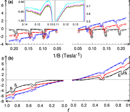
Figure 3: (Color online) (a) Spin polarization as a function of $1/B$. The results for $r=0,0.2,0.4$ are shown in black, red and blue. Insets: Perturbed spin polarizations for $r=g^{\ast}=0.2$ at $\delta=0.2,0.4,0.8$ are shown in green, pink and cyan. (b) Spin polarization as a function of $r$. The results for $\nu_{F}=1.0,2.0,3.0$ are shown in black, red and blue. In both figures, right panel: negative edge; left panel: positive edge, $n_{e}=5\times 10^{11}\text{cm}^{-2}$ and the solid, dash-dot lines indicate the results for $g^{\ast}=0.2,0.4$.

For $r=0$ we reproduce the well-known results for the usual 2DEG in which the electrons are magnetized by the Zeeman interaction with only very small negative spin polarization accumulated near both edges. In this case the spin polarization oscillates with $1/B$ with almost constant amplitude. This oscillation pattern is nothing but the Shubnikov-de Hass (SdH) oscillation with the period $\Delta_{\text{SdH}}(1/B)=1/(\Phi_{0}n_{e})$ where $\Phi_{0}=h/e$ is the flux quantum. For $n_{e}=5\times 10^{11}\;\text{cm}^{-2}$ Sih et al. (2005), our analytic calculation gives a period of $0.048\;(\text{T}^{-1})$ which is in precise agreement with our numerical data. Interestingly, when the SOC constant, positive for example, is turned on adiabatically, although the SdH oscillation remains with the same period, its amplitude is no longer constant but changes in different way with $1/B$ for opposite edges. Near the negative edge the amplitude increases from negative to positive with the decreasing of the magnetic field, while near the positive edge the amplitude not only remains negative but also decreases further. Moreover, as we further increase $r$, more up (down) spins are pumped to the negative (positive) edge due to the larger non-Abelian gauge flux. As an example, the spin polarization for $r=0.2$ and 0.4 are shown in color in Fig. 3(a), among which the results in red correspond to the experimental parameters for AlGaAs [110] QWs Sih et al. (2005). To have an overview of the dependence of the spin polarization on the SOC constant, we also plot in Fig. 3(b) the spin polarization as a function of $r$ at the Fermi energies $\nu_{F}=1.0,2.0,3.0$ respectively, the result of which shows clearly that the larger the SOC constant is, the more positive (negative) the spin polarization near the negative (positive) edge is. Furthermore, there is a similar oscillation pattern with increasing $r$, where the turning point $r_{\sigma}$ occurs whenever the gauge flux changes to the values so that the Fermi energy for spin $\sigma$ crosses a bulk LL $\nu_{F\sigma}=n$, and the period of which is given by $\Delta r^{2}(\Phi_{\sigma})|_{r_{\sigma}}=1/2$. This periodicity corresponds exactly to the Aharonov-Bohm period for both down and up spin components of the gauge flux. For negative SOC constant the same results are obtained with only the sign-exchange of the spin polarization between the boundaries. The above results present an interesting scenario for the spin accumulation: electrons with opposite out-of-plane spin components accumulate near the opposite edges, the relative sign of which can be tuned by the sign of the SOC constant; by decreasing the magnetic field or increasing the SOC constant and/or the electron density, the magnitude of the spin polarization can be enlarged greatly compared to the equilibrium case.

This phenomenon is a direct result of the intrinsic electric $SU(2)$ gauge field in our system. Mathematically it is clearly seen through the expression of $y_{0\sigma}$ that for fixed $l_{b}$ the adiabatical increasing of $r$ (positive) moves the orbital centers of up spin to negative $y$ direction, and in the meanwhile carries those of down spin to positive $y$ direction. The same conclusion is reached through similar analysis when decreasing the magnetic field for fixed $r$. To have an idea of the magnitude of the spin accumulation in real materials, we recall that the range of the SOC constants from weak to strong is Bernevig et al. (2006) $10^{-13}\rightarrow 10^{-11}\;\text{eV}\cdot\text{m}$ corresponding approximately to $r\in(0,0.5)$ which is covered by our results shown in Fig. 3.

Let’s now turn our attention to the charge and spin current as well as their Hall conductance. The charge current operator for each spin component is given by $j_{x\sigma}^{c}=-ev_{x\sigma}$ where $v_{x\sigma}=\frac{\partial H_{0\sigma}}{\partial p_{x}}$ is the velocity operator. The total charge current is the sum of that from up and down spin components $I_{x}^{c}(r)=e\omega_{c}l_{b}\int d\widetilde{y}\sum_{nk\sigma}^{\nu_{F\sigma}}(\widetilde{y}+\widetilde{y}_{0}+2r\sigma)|\phi_{nk\sigma}|^{2}$, and the charge Hall conductance (CHC) follows $G^{c}_{xy}=G^{c}_{xy,+}+G^{c}_{xy,-}$. To compare we also consider the spin current polarized in $z$ direction flowing along the edges by taking the traditional definition $j^{s}_{x}=\frac{\hbar}{4}\{v_{x},\sigma_{z}\}=-(\hbar/2e)j_{x}^{c}\sigma_{z}$, where we see that in our system this spin current is physically just the $\sigma_{z}$-carrying charge current. Therefore the definition of spin current is physically meaningful here in the sense that it satisfies a well-behaved continuity equation since the charge current does, so there is no controversy on the conservation issue which usually can’t be avoided in general SOC systems. Different from that of charge current, the total spin current is given by the difference of the currents from up and down spin components $I^{s}_{x}(r)=I^{s}_{x+}(r)-I^{s}_{x-}(r)$ and so as the spin Hall conductance (SHC) $G^{s}_{xy}=G^{s}_{xy,+}-G^{s}_{xy,-}$. Our numerical results for CHC and SHC at the parameters $r=g^{\ast}=0.2$ close to those for AlGaAs [110] QWs Sih et al. (2005) are shown in Fig. 4, it is seen that for CHC there are wider steps when it is quantized in even multiples of the quantum of conductance, while the steps are much narrower when it is quantized in odd multiples of the quantum of conductance. For SHC they are non-vanishing only when the CHC takes odd integers and the corresponding quantized number is unity.

The above results can be easily understood by the standard argument MacDonald and Středa (1984) that the charge current flows only if there exists a chemical potential difference between the edges, and whenever the current flows CHC is quantized in units of $e^{2}/h$ with the quantized number being the number of edge states occupied. In our system, for each spin component we have $G^{c}_{xy,\sigma}=n+1$ with $\nu_{F\sigma}\in(\nu^{\text{edge}}_{n-},\nu^{\text{edge}}_{n+1,-})$, and the total CHC takes even or odd integers depending on the relative fillings of the LLs by up and down spin. The quantization of SHC is a direct result of the quantization of the CHC of a spin-polarized LL in the presence of the Zeeman splitting at odd integer filling factor. It is obvious from the relation between the charge and spin current operators that the SHC for each spin component is quantized in units of $-e/4\pi$ with the quantized number equals to that of the CHC, hence it is nonvanishing only when the total CHC takes odd integers otherwise different spin components will cancel each other giving zero. The width of the odd steps is $\Delta(1/B)=g^{\ast}\Delta_{\text{SdH}}/2$ which equals approximately to $0.0048\;(\text{T}^{-1})$ for the parameters taken in Fig. 4. It is worth noting that in a previous work by Bao et al. Bao et al. (2005), similar results for charge and (resonant) spin Hall conductance are first obtained in a general model with both Rashba and Dresselhaus SOC, where the SHC is not quantized and the spin accumulation decays due to the diffusive property in these systems.

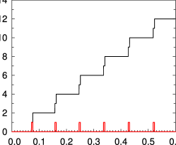
Figure 4: (Color online) Quantized charge and spin Hall conductance as a function of $1/B$. The CHC and SHC are shown respectively as black and red lines. The parameters are taken as $r=0.2,\;g^{\ast}=0.2,\;n_{e}=5\times 10^{11}\text{cm}^{-2}$.

Finally we discuss the Rashba-type perturbation term $H_{R}=\delta\beta[p_{y}\sigma_{x}-(\hbar k-eBy)\sigma_{y}]/\hbar$, where the Rashba SOC constant has been written as $\alpha=\delta\beta$ with $\delta$ being a small perturbation number. This Hamiltonian couples the LLs of different spin components and the wavefunction perturbed to the first order of $H_{R}$ gives

$$\Phi_{nk\sigma}=\phi_{nk\sigma}+\sum_{n^{\prime}}\frac{W_{n^{\prime}k\overline{\sigma};nk\sigma}}{E_{nk\sigma}-E_{n^{\prime}k\overline{\sigma}}}\phi_{n^{\prime}k\overline{\sigma}},$$ (4)

where $E_{nk\sigma}-E_{n^{\prime}k\overline{\sigma}}=\hbar\omega_{c}\left[\nu_{n\sigma}-\nu_{n^{\prime}\overline{\sigma}}+g^{\ast}(\sigma-\overline{\sigma})/4\right]$ and $W_{n^{\prime}k\overline{\sigma};nk\sigma}=\int d\widetilde{y}\phi^{\ast}_{n^{\prime}k\overline{\sigma}}(\widetilde{y})H_{R,\overline{\sigma}\sigma}(\widetilde{y},\partial_{\widetilde{y}})\phi_{nk\sigma}(\widetilde{y})$ with $\bar{\sigma}=-\sigma$. We have studied systematically the effect of the perturbations to the spin polarization and some of the results are shown as insets in Fig. 3(a). It is concluded that the perturbations in general make the spin polarization more positive at both edges so that $\langle\sigma_{z}(r)\rangle$ is increased near negative edge while decreased near positive edge, and the larger $\delta$ and/or $r$ is the more the increases (decreases) are. But in general the magnitude of these deviations is very small and will not qualitatively change our picture of the spin accumulation.

We propose to use Kerr measurements to detect our predictions on spin accumulation. It is calibrated in the experiment Kato et al. (2004) that for the film-like 3d sample, the spin density of 20 Bohr magnetons per $\mu\text{m}^{-3}$ is signaled by $1\;\mu\text{rad}$ of Kerr rotation angle. Bearing in mind that the film thickness used in the experiment $l=0.6\;\mu\text{m}$ is 2 to 3 orders smaller than the other two dimensions, hence a similar correspondence can be estimated for quasi-2d systems that the spin density of 10 Bohr magnetons per $\mu\text{m}^{-2}$ lead to $1\;\mu\text{rad}$ of Kerr rotation angle. For the parameters of AlGaAs [110] QWs Sih et al. (2005) used in our calculation, the spin density $n_{s}=\langle\sigma_{z}\rangle/l_{b}^{2}$ is estimated to be $10^{4}$ Bohr magnetons per $\mu\text{m}^{-2}$ at $B=5\;\text{T}$, which is several orders above the state-of-art detection limit in the experiment Kato et al. (2004), and our predicted spin accumulation can be easily detected within the available experimental sensitivities.

We wish to thank Drs Ruibao Tao, Shun-Qing Shen, Xiao-Liang Qi, Xi Dai, Zhong Fang, Xiao-Feng Jin and Yuan Tian for helpful discussions. This work is supported by MOE of China under the grant number B06011, and by the NSF under grant numbers DMR-0342832 and the US Department of Energy, Office of Basic Energy Sciences under contract DE-AC03-76SF00515.

References

- Murakami et al. (2003) S. Murakami, N. Nagaosa, and S.-C. Zhang, Science 301, 1348 (2003).
- Sinova et al. (2004) J. Sinova, D. Culcer, Q. Niu, N. A. Sinitsyn, T. Jungwirth, and A. H. MacDonald, Phys. Rev. Lett. 92, 126603 (2004).
- Kato et al. (2004) Y. K. Kato, R. C. Myers, A. C. Gossard, and D. D. Awschalom, Science 306, 1910 (2004).
- Wunderlich et al. (2005) J. Wunderlich, B. Kaestner, J. Sinova, and T. Jungwirth, Phys. Rev. Lett. 94, 047204 (2005).
- Bernevig et al. (2006) B. A. Bernevig, J. Orenstein, and S.-C. Zhang, Phys. Rev. Lett. 97, 236601 (2006).
- Weber et al. (2007) C. P. Weber, J. Orenstein, B. A. Bernevig, S.-C. Zhang, J. Stephens, and D. D. Awschalom, Phys. Rev. Lett. 98, 076604 (2007).
- Laughlin (1981) R. B. Laughlin, Phys. Rev. B 23, 5632 (1981).
- Halperin (1982) B. I. Halperin, Phys. Rev. B 25, 2185 (1982).
- Jin et al. (2006) P.-Q. Jin, Y.-Q. Li, and F.-C. Zhang, J. Phys. A 39, 7115 (2006).
- MacDonald and Středa (1984) A. H. MacDonald and P. Středa, Phys. Rev. B 29, 1616 (1984).
- Sih et al. (2005) V. Sih, R. C. Myers, Y. K. Kato, W. H. Lau, A. C. Gossard, and D. D. Awschalom, Nature Phys. 1, 31 (2005).
- Bao et al. (2005) Y.-J. Bao, H.-B. Zhuang, S.-Q. Shen, and F.-C. Zhang, Phys. Rev. B 72, 245323 (2005).