Spin solid phases of spin $1$ and spin $3/2$ antiferromagnets on a cubic lattice.

Abstract

We study spin $S=1$ and $S=3/2$ Heisenberg antiferromagnets on a cubic lattice focusing on spin solid states. Using Schwinger boson formulation for spins, we start in a $U(1)$ spin liquid phase proximate to Neel phase and explore possible confining paramagnetic phases as we transition away from the spin liquid by the process of monopole condensation. Electromagnetic duality is used to rewrite the theory in terms of monopoles. For spin $1$ we find several candidate phases of which the most natural one is a phase with spins organized into parallel Haldane chains. For spin $3/2$ we find that the most natural phase has spins organized into parallel ladders. As a by-product, we also write a Landau theory of the ordering in two special classical frustrated XY models on the cubic lattice, one of which is the fully frustrated XY model. In a particular limit our approach maps to a dimer model with $2S$ dimers coming out of every site, and we find the same spin solid phases in this regime as well.

I Introduction

A simple, nontrivial, and physically common example of a regular system of quantum objects is a collection of spins on a lattice. This is easiest to analyze if the interactions do not compete and all prefer the same spin state; the resulting phases have been known for a long time and include ferromagnetic and Neel states. A much richer situation of current interest is when interactions compete. The frustration together with quantum fluctuations can destroy the magnetic order and produce spin solid or spin liquid phases. In a spin solid, spins combine into larger singlet objects such as valence bonds which form an ordered pattern on a lattice. Such phases have been found in nature,Taniguchi ; Chow ; Kageyama and also in numerical studies of model Hamiltonians.Sandvik ; Beach ; Harada A spin liquid, on the other hand, is a featureless paramagnet, which can be crudely viewed as a quantum superposition of many valence bond configurations, thus the name “resonating valence bonds” (RVB) state. So far there are only few experimental candidates, but on the theoretical side the existence of spin liquids in many varieties and our understanding of them is well established (see Ref. Banerjee, for a recent collection of references and also a very recent example of the so-called Coulomb phase in 3d, which is the spin liquid relevant to the present work).

In this paper we look for natural spin solid phases of spin $1$ and spin $3/2$ on a cubic lattice. A direct study of spin Hamiltonians that can stabilize such phases is difficult but can be done in some cases with Quantum Monte Carlo. Which phases are realized will of course depend on the specific model: For example, Refs. Sandvik, ; Beach, found valence bond solids in spin 1/2 systems with ring exchanges on the square and cubic lattices. Refs. Harada, ; Harada3d, found spin solid phases for a spin 1 model with biquadratic interaction on the anisotropic square lattice, but only magnetically ordered phases on the isotropic square and cubic lattices.

Here we follow instead a more phenomenological approach. Arovas ; ReadSachdev ; Haldane ; MotrunichSenthil A systematic and commonly used route to achieve this, and the one we start with, is to generalize the spins to a representation of higher symmetry group, here taken to be $SU(N)$.Arovas ; ReadSachdev The problem can be solved exactly in the $N\to\infty$ limit and one can consider fluctuations around this limit to get long distance properties of the system. This approach, while difficult to connect with the actual microscopic $SU(2)$ spin system, nevertheless gives us some guidance about what phases to expect and gives us a form of the effective field theory. Here it results in a gauge theory which naturally exhibits deconfined (liquid) and confined (solid) phases, and we expect that if a microscopic spin system has such phases, they should be described by this theory.

Figure 1: The most natural spin solid phase for $S=1$ on the cubic lattice. The thick lines denote links with large spin-spin correlations suggesting that the spins organize into Haldane chains along one lattice direction.

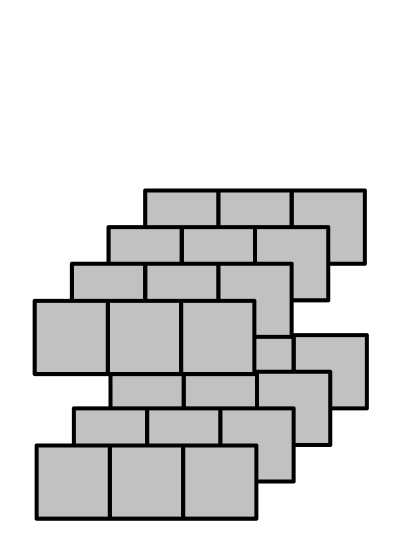
Figure 2: The most natural spin solid phase for $S=3/2$ on the cubic lattice. The drawn bold lines denote links with large spin-spin correlations suggesting that the spins organize into ladders.

One of the spin liquid phases expected in 3d is the so-called Coulomb phase. It is a compact $U(1)$ gauge theory coupled to matter in the deconfined phase, where the matter fields (spinons) are gapped, gauge field (emergent photon) is gapless, and monopoles (which arise due to compactness) are gapped. In addition, importantly, there are spin Berry phases that lead to the presence of a background charge in the gauge theory formulation. This makes the confined phases nontrivial in that they break lattice symmetries and therefore correspond to various spin solids. The transition occurs because the monopoles condense, and the theory can be equivalently analyzed in terms of them by employing standard electro-magnetic duality. The background charge causes monopoles to acquire a phase when they hop around a plaquette.MotrunichSenthil This leads to a nontrivial monopole condensation pattern, which then corresponds to a spin solid phase. In 2d the physics is similar, except that the monopoles are instantons and they always proliferate, so there is no Coulomb spin liquid. This approach was first used by Read and SachdevReadSachdev on the square lattice. The spin solids for spin 1/2 on the cubic lattice were analyzed in Ref. MotrunichSenthil, and near several different Coulomb spin liquids in Ref. Bernier, . Ref. Bergman, was led (in a different context) to a gauge theory with background charges on a diamond lattice which was attacked using analogous techniques.

For the spins on the cubic lattice, the analysis depends only on the spin magnitude. Any case can be mapped onto $S=0$, $1/2$, and $1$ in 2d and $S=0$, $1/2$, $1$, and $3/2$ in 3d. Only the spin 1/2 case was considered so far, but these results cannot be transferred to the other spins since each requires a separate analysis. This is the task of the present work. We find that the most natural phases for spin $1$ and $3/2$ are the ones shown on Figures 1 and 2. In the $S=1$ case the spins organize into Haldane chains. This is easiest to understand in the standard picture where we break spin $1$ into two spin $1/2$’s and form singlets with spin $1/2$’s of spins on either side. Similarly, in the $S=3/2$ case we break spin $3/2$ into three spin $1/2$’s and form singlets on the bonds of the ladders. Several approaches that we have taken and used in different parameter regimes suggest the same spin solid states, which gives us confidence that these phases are very natural in the two cases.

II Schwinger bosons, dual reformulation, and a basic phase diagram

II.1 Schwinger bosons

We begin by briefly reviewing the standard technique of large $N$ for spins.ReadSachdev ; Arovas This maps (approximately) our spin system into a theory of spinons coupled to a $U(1)$ gauge field in the presence of static background charges. Our main work is the analysis of this theory, while the purpose of the review here is to establish the connection with the properties of the original spin system.

The basic steps in the derivation are as follows. We generalize the $SU(2)$ spin to $SU(N)$ spin and denote it by $S^{\beta}_{\alpha}(i)$. We write the spins in terms of Schwinger bosons:

$$S^{\beta}_{\alpha}(i) = b^{\dagger}_{\alpha}(i)b^{\beta}(i)~{}~{}\mbox{sublattice A}~{},$$

$$S^{\beta}_{\alpha}(j) = -\bar{b}^{\beta\dagger}(j)\bar{b}_{\alpha}(j)~{}~{}\mbox{ sublattice B}~{},$$ (1)

where the $b,\bar{b}$’s are bosonic operators that transform under the fundamental representation of $SU(N)$ if the index is on the top and under its conjugate if the index is on the bottom. To get the Hilbert space of the spins we need to restrict the boson occupations as

$$b^{\dagger}_{\alpha}(i)b^{\alpha}(i) = n_{c}~{},$$

$$\bar{b}^{\alpha\dagger}(j)\bar{b}_{\alpha}(j) = n_{c}~{},$$ (2)

where $n_{c}$ corresponds to the spin length. The $SU(N)$ spin Hamiltonian is

$$H=\frac{J}{N}\sum_{\langle i,j\rangle}S^{\beta}_{\alpha}(i)S^{\alpha}_{\beta}(j)~{},$$ (3)

which reduces to the $SU(2)$ Heisenberg spin model for spin $S$ when $N=2$ and $n_{c}=2S$.

Next we write the system in the path integral picture, imposing the constraints (2) by Lagrange multipliers. The spin interaction contains quartic terms; to get action that is quadratic in the boson fields, we use Hubbard-Stratonovich transformation and obtain

$${\cal L} = \sum_{i}b^{\dagger}_{\alpha}(i)\left(\frac{\partial}{\partial\tau}+i\lambda(i)\right)b^{\alpha}(i)-i\lambda(i)n_{c}$$ (4)

$$+\sum_{j}\bar{b}^{\alpha\dagger}(j)\left(\frac{\partial}{\partial\tau}+i\lambda(j)\right)\bar{b}_{\alpha}(j)-i\lambda(j)n_{c}$$

$$+\sum_{\langle i,j\rangle}\frac{N}{J}|Q_{ij}|^{2}-Q_{ij}^{*}b^{\alpha}(i)\bar{b}_{\alpha}(j)+h.c.$$

The path integral goes over $b,\bar{b},Q,\lambda$.

We can now integrate out the $b$’s. The resulting expression will have coefficient $N$ in front of it. At large $N$ it can be approximated by its saddle point value. Our departing point is such a “mean field” with uniform $Q_{r,r+\hat{m}}(\tau)=\bar{Q}$ and $\lambda(r,\tau)=\bar{\lambda}$ and assuming gapped $b$ spectrum; this represents a Coulomb spin liquid, which is a stable phase in three dimensions. The effective theory is obtained by considering the fluctuations of the fields, $Q_{r,r+\hat{m}}(\tau)=[\bar{Q}+q_{m}(r,\tau)]e^{i\alpha_{m}(r,\tau)}$ and $\lambda(r,\tau)=\bar{\lambda}+i\alpha_{0}(r,\tau)$. Here $r$ runs over all sites of the cubic lattice and $\hat{m}=\hat{x},\hat{y},\hat{z}$ denotes one of the directions in 3d. The amplitude fields $q_{m}$ are massive, and so are the fields $\alpha_{m}$ and $\alpha_{0}$ near the wavevector $(0,0,0)$. On the other hand, the fields $\alpha_{m}$ and $\alpha_{0}$ near the wavevector $(\pi,\pi,\pi)$ are massless and describe the gauge field (photon) of the Coulomb phase, $a_{m}\equiv\alpha^{(\pi,\pi,\pi)}_{m}$, $a_{\tau}\equiv\alpha_{0}^{(\pi,\pi,\pi)}$. For details of the derivation, see the original Ref. ReadSachdev, (our notation is slightly different compared to these papers, which use a two-site unit cell labeling instead).

As emphasized in Refs. ReadSachdev, ; Haldane, , we also have to consider effect of Berry phases, which is crucial for the understanding of the spin solid states. A very convenient encapsulation of the low-energy degrees of freedom and the Berry phases is provided by the following re-latticized Euclidean action:SachdevJalabert ; SachdevPark

$$Z = \int_{-\pi}^{\pi}Da_{i\mu}e^{-S_{a}-S_{B}}~{},$$ (5)

$$S_{a} = -\beta\sum_{i,\mu<\nu}\cos(\nabla_{\mu}a_{\nu}-\nabla_{\nu}a_{\mu})~{},$$

$$S_{B} = i\sum_{i}\eta_{i}a_{i\tau}~{}.$$

Here we have a compact $U(1)$ gauge field $a$ residing on the links of a (3+1)d space-time lattice and described by the action term $S_{a}$. The $S_{B}$ term comes from detailed consideration of the Berry phases, and $\eta_{i}$ is $2S$ on one sublattice of the spatial lattice and $-2S$ on the other one. In the Hamiltonian language this has a simple interpretation as a background charge of value $2S$ on one sublattice and $-2S$ on the other one:

$$H=u\sum_{r,m}E_{rm}^{2}-\kappa\sum_{r,m<n}\cos(\nabla_{m}a_{n}-\nabla_{n}a_{m})~{},$$ (6)

$$(\nabla\cdot E)_{r}=\eta_{r}=\pm 2S~{},$$ (7)

where $E_{m}$ are electric fields residing on the links of the 3d cubic lattice and conjugate to $a_{m}$. Thus we obtained a compact $U(1)$ gauge theory in the presence of background charge.ZhengSachdev ; FradkinKivelson ; FradkinBook

Throughout, we will assume the spinons are gapped and are integrated out. Note that even though we start in the Coulomb phase where the gauge field is deconfined, the above action also provides access to confining paramagnetic phases, and this will be our main focus. To sum up, we will be describing spin solid phases that are proximate to the simple Coulomb phase; the latter with the specified Berry phases encoded in the staggered background charge is in turn appropriate in the vicinity of the conventional Neel phase.

Since we will continue with (5) we need a way to connect the variables there to the original spin variables. This is done as follows. The nearest neighbor spin-spin correlation $\langle{\bf S}_{r}\cdot{\bf S}_{r^{\prime}}\rangle$ is proportional to the bond variable $|Q_{rr^{\prime}}|^{2}$. To get the connection between the fluctuation of the magnitude of $Q$ and the gauge fields we have to also keep the massive amplitude fields $q_{m}$ in the above derivation when integrating out the $b$’s. One finds that the $(\pi,\pi,\pi)$ component couples to the gauge fields in the action as follows: $\delta S=i\gamma\sum q^{(\pi,\pi,\pi)}_{m}(\partial_{m}a_{\tau}-\partial_{\tau}a_{m})$, with some coupling parameter $\gamma$. On the other hand, in the derivation of the path integral from the Hamiltonian formulation of the gauge theory, the electric field is coupled to the gauge field in the same way, i.e., via a term $i\sum E_{m}(\partial_{m}a_{\tau}-\partial_{\tau}a_{m})$ in the action. Thus the electric field gives the fluctuation of the staggered nearest neighbor spin-spin correlation function.

II.2 Electro-magnetic duality

We now proceed to the analysis of the model (5). We are interested in the confining phases, which will necessarily break lattice symmetries for spins $S=1/2,1,3/2$ studied here. The confinement occurs due to condensation of monopoles. Therefore we would like to express the theory in terms of them. This can be done by the standard electro-magnetic duality. The duality maps the theory of a compact $U(1)$ gauge field without charges into a theory of a noncompact gauge field coupled to charges – the monopoles of the original theory. The noncompactness comes from the fact that we have dropped the electric charges in the original theory; had we retained them, we would have obtained a compact dual gauge field whose monopoles would correspond to the original charges. The new variables reside on the lattice dual to the original lattice. The background charge of the original theory gives rise to a static dual magnetic flux emanating out of the center of each cube as drawn in Figure 3. This flux alternates in sign from one cube to the next and frustrates the monopole hopping. Therefore we obtain a theory of monopoles with frustrated hopping that are coupled to the dual noncompact gauge field.MotrunichSenthil The duality can be done explicitly with various approximations clearly displayed as is written in Appendix A.

Explicitly, the partition function is

$$Z \sim \int_{-\pi}^{\pi}D\theta\int_{-\infty}^{\infty}DL\,\,e^{-S_{\rm dual}}~{},$$ (8)

$$S_{\rm dual} = \sum\frac{(\partial L)^{2}}{8\pi^{2}\beta}-\sum\lambda\cos(L+L^{0}-\nabla\theta)~{},$$ (9)

where $L$ is the dual gauge field, $(\partial L)_{\mu\nu}=\nabla_{\mu}L_{\nu}-\nabla_{\nu}L_{\mu}$ is the four dimensional curl, $L^{0}$ is the frustration that results from the original background charge and ultimately from Berry phases, and $\theta$ is the monopole field. A convenient choice of $L^{0}$ that produces the appropriate static fluxes is shown in Figure 3; all subsequent work is done in this gauge.

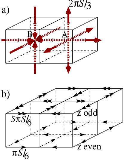
Figure 3: a) Original background electric charges $2S$ and $-2S$ on the two sublattices give rise to the static dual magnetic fluxes as seen by the monopoles. b) Gauge choice for $L^{0}$ that realizes these fluxes modulo $2\pi$.

The advantage of the dual formulation is that it has no sign problem and can be in principle studied by Monte Carlo. A sketch of the phase diagram is on Figure 4. In the bottom left side of the diagram, the monopoles are gapped and the system is in the deconfined phase, which correspond to the Coulomb spin liquid in the spin model. At large enough $\lambda$ and $1/\beta$, the monopoles condense. They can condense in various patterns which translate to various spin solid phases of the original model. Duality relates the original field theory (5) to the large $\lambda$ part of the dual theory. It is hard to analyze the transition in the large $\lambda$ limit. Instead we look at three different places in this phase diagram. At $1/\beta=\infty$ the system becomes frustrated XY model. First we analyze the phase transition looking for ordering of the XY spins as we cross the phase boundary to the ordered phase. This gives us the most likely monopole condensation patterns near the transition. Next we look at the classical ground state of the XY model in the upper right corner of the phase diagram as approached from $1/\beta=\infty$. Finally we look near the same point but in the limit $\lambda\gg 1/\beta$.

Figure 4: Sketch of the expected phase diagram for the dual action Eq. (9).

III Analysis 1,2: frustrated XY model at $1/\beta=\infty$

III.1 Outline of the Analysis

In this section we describe in general terms the analysis in the $1/\beta=\infty$ limit where the dual action Eq. (9) reduces to a frustrated XY model. We look at the phase transition and the classical ground state.

In the Analysis 1, we consider the transition in the spirit of the Landau theory. We identify the relevant low-energy fields, write the most general quartic potential consistent with the symmetries, and study it in mean field. The approach is the same for each spin $S$, but the details are unique in each case and are contained in Subsections III.2 and III.3 for spin 1 and spin 3/2 respectively (spin 1/2 was considered using this approach in Ref. MotrunichSenthil, ).

More explicitly, the mean field derivation is done as follows. The mean field theory of XY spins is described by the continuous soft spin action

$$\int d\tau\left[\sum_{R}|\partial_{\tau}\Phi_{R}|^{2}-\sum_{\langle RR^{\prime}\rangle}(t_{RR^{\prime}}\Phi_{R}^{*}\Phi_{R^{\prime}}+c.c.)+\sum_{R}V(|\phi_{R}|^{2})\right]$$ (10)

with some potential $V(|\Phi_{R}|^{2})=r_{0}|\Phi_{R}|^{2}+u_{0}|\Phi_{R}|^{4}+\cdots$. After crossing the transition from the disordered side, the system enters a phase with non-zero $\Phi_{R}$ that minimize this action. The initial step is to minimize the kinetic energy. This will turn out to have a three-dimensional manifold of minima for spin 1 and four-dimensional one for spin 3/2. One then expands around these minima and writes all terms to a given order that are allowed by symmetry. In both cases the degeneracy is lifted at the fourth order. We will find that for spin 1 there are three independent quartic terms and we manage to draw a general phase diagram of the Landau theory. For spin 3/2, there are five such terms and the parameter space is too rich for us to describe the phase diagram completely. In this case we confine ourselves to examining the potential obtained from the most natural microscopic fourth order term and determining its mean field phase.

In the Analysis 2, we find the classical ground state of the frustrated XY model – the state in the upper right point of the phase diagram Figure 4 – by a direct minimization of the hard-spin action (9). We use the following method: For some system size, we start with a random configuration of spins. We pick a random spin and minimize its (local) energy and repeat this process until the total energy converges. Different starting configurations will lead to different final energies, because sometimes the system gets stuck in some local minima. We repeat this procedure for many starting configurations and also for different system sizes. We then select the configurations with the same lowest energy, which gives the absolute minimum of the potential. The case of spin 3/2, which corresponds to a fully frustrated XY model, was already considered some time ago in Ref. Diep, , and our method produces results in agreement with that work.

For both spin 1 and spin 3/2, we find that the classical ground state coincides with the most natural state identified in the mean field theory near the transition. This suggests that there is only one XY-ordered phase along the $1/\beta=\infty$ line in Fig. 4, which could in principle be tested in Monte Carlo studies of the corresponding frustrated XY models.

We have described how to find the phases of the dual action in the $1/\beta=\infty$ limit. However we are interested in the phases of the original spin model. To make the connection we calculate the energies and staggered curls of the monopole currents in the dual model and relate them to variables in the original spin problem. These variables are the plaquette energy and the bond expectation value respectively. This allows us to determine the spin solid patterns.

The mapping of the first variable, the energy, is simple. Energy simply maps to energy. In the dual model we can calculate the energy for each bond, which is $\epsilon=2{\rm Re}(t_{RR^{\prime}}\Phi^{*}_{R}\Phi_{R^{\prime}})$. The center of a bond of the dual lattice coincides with the center of a plaquette of the original lattice, and so the calculated energy is the plaquette energy of the original model.

The connection of the staggered curls of the monopole current to the original bond variables is established as follows. The monopole current is given by $J_{M}=2{\rm Im}(t_{RR^{\prime}}\Phi^{*}_{R}\Phi_{R^{\prime}})$. In terms of the original gauge theory, Eq. (5), just as the electric current produces magnetic field, the magnetic current produces electric field. The resulting electric field is given by the analog of Biot-Savart law. However, approximately, if we have a loop of the magnetic current, the electric field it produces in the center is proportional to the circulation of the current, which is what we call the curl of the monopole current. As we described in the preceding section, the electric field is proportional to the staggered fluctuation of the nearest neighbor spin-spin correlation function, therefore the claimed connection. We will use this extensively in the detailed treatment of spin 1 and spin 3/2 below.

III.2 Results: Spin 1

III.2.1 Analysis 1: Phase transition of the XY model

Now we turn to finding the phases for spin 1. We choose the gauge shown on Figure 3. In this case the hopping amplitudes in (10) are given by

$$t_{R,R+\hat{x}} = \frac{1}{2}\left[(-1)^{z}\sqrt{3}+i(-1)^{x+y}\right]~{},$$ (11)

$$t_{R,R+\hat{y}} = \frac{1}{2}\left[(-1)^{z}\sqrt{3}-i(-1)^{x+y}\right]~{},$$ (12)

$$t_{R,R+\hat{z}} = 1~{}.$$ (13)

The band structure has three minima and hence the space of ground states of the kinetic energy is three dimensional. Convenient choice of the basis is the following:

$$\Psi_{1} = \frac{(-1)^{x+y+z}-(-1)^{x+y}\sqrt{3}+i[(-1)^{z}+\sqrt{3}]}{2\sqrt{2}}~{},$$

$$\Psi_{2} = i\frac{(-1)^{x+y+z}-(-1)^{x+y}\sqrt{3}-i[(-1)^{z}+\sqrt{3}]}{2\sqrt{2}}~{},$$

$$\Psi_{3} = -\,\frac{(-1)^{y}+i(-1)^{x}}{\sqrt{2}}~{}.$$

A general kinetic energy ground state can be written as

$$\Phi(R)=\phi_{1}\Psi_{1}(R)+\phi_{2}\Psi_{2}(R)+\phi_{3}\Psi_{3}(R)$$ (14)

with complex fields $\phi_{1,2,3}$. This degeneracy will be lifted by nonlinear terms. To find out how, we would like to write the Landau theory for the $\phi$’s, including all terms that are allowed by symmetry. Thus we need to find how the $\phi$’s transform under the lattice symmetries.

The generators of the symmetries are the translations by one lattice spacing in the x,y,z directions, 90 degree rotations around the x,y,z axes (it suffices to consider two out of three rotations), and mirror reflections. Note that the fluxes seen by the monopoles (and encoded in the complex phases of the hopping amplitudes $t_{RR^{\prime}}$) change sign under unit translations. The original spin problem is translationally invariant, and this is represented in the dual action (10) as follows. The fluxes remain unchanged if the $t$’s are also conjugated after the translation, and there is a gauge transformation that brings such modified $t$’s to the original themselves. The action of the symmetry on the field $\Phi$ is then a combined application of the translation of the coordinates, conjugation, and gauge transformation. Similar considerations apply for the 90 degree rotations performed here about the dual lattice axes. After carrying through this analysis, the transformation properties of $\phi$’s are remarkably simple:
$T_{x}$ $T_{y}$ $T_{z}$ $R_{x}$ $R_{y}$ $R_{z}$ $\phi_{1}\to$ – + + + $\phi_{3}^{*}$ $\phi_{2}^{*}$ $\phi_{2}\to$ + – + $\phi_{3}^{*}$ + $\phi_{1}^{*}$ $\phi_{3}\to$ + + – $\phi_{2}^{*}$ $\phi_{1}^{*}$ +


In this table, “$+$” or “$-$” stands for $\phi_{i}\to\phi_{i}^{*}$ or $\phi_{i}\to-\phi_{i}^{*}$ respectively. We see that $\phi_{1}$ can be loosely associated with the $x$ direction, $\phi_{2}$ with $y$, and $\phi_{3}$ with $z$. We should also point out that under mirror symmetries in the dual lattice planes the fields transform simply $\phi_{i}\to\phi_{i}$.

There is only one invariant term at the quadratic level:

$$V^{(2)}=m(|\phi_{1}|^{2}+|\phi_{2}|^{2}+|\phi_{3}|^{2})~{},$$ (15)

where $m$ is a constant. There are three independent allowed terms at the quartic level, and the most general quartic potential can be written in the form

$$V^{(4)} = u(|\phi_{1}|^{2}+|\phi_{2}|^{2}+|\phi_{3}|^{2})^{2}$$ (16)

$$+ v(|\phi_{1}|^{4}+|\phi_{2}|^{4}+|\phi_{3}|^{4})$$

$$+ w(\phi_{1}^{*2}\phi_{2}^{2}+\phi_{2}^{*2}\phi_{3}^{2}+\phi_{3}^{*2}\phi_{1}^{2}+c.c.)~{},$$

where $u$, $v$, $w$ are constants.

To find the phases of the Landau theory, we simply need to minimize this potential. Before we start describing the phases, however, it is useful to introduce bilinears of the fields. The reason is that these are gauge independent objects whereas the form of $\Psi_{1,2,3}$ and hence the transformation properties of $\phi_{1,2,3}$ are gauge dependent. We consider the following bilinears:

$$B_{0} = |\phi_{1}|^{2}+|\phi_{2}|^{2}+|\phi_{3}|^{2}~{},$$

$$F_{1} = \frac{1}{\sqrt{3}}(|\phi_{1}|^{2}+|\phi_{2}|^{2}-2|\phi_{3}|^{2})~{},$$

$$F_{2} = |\phi_{1}|^{2}-|\phi_{2}|^{2}~{},$$

$$D_{x} = \phi^{*}_{3}\phi_{2}+\phi^{*}_{2}\phi_{3}~{},$$

$$D_{y} = \phi^{*}_{1}\phi_{3}+\phi^{*}_{3}\phi_{1}~{},$$

$$D_{z} = \phi^{*}_{2}\phi_{1}+\phi^{*}_{1}\phi_{2}~{},$$

$$N_{x} = i(\phi^{*}_{3}\phi_{2}-\phi^{*}_{2}\phi_{3})~{},$$

$$N_{y} = i(\phi^{*}_{1}\phi_{3}-\phi^{*}_{3}\phi_{1})~{},$$

$$N_{z} = i(\phi^{*}_{2}\phi_{1}-\phi^{*}_{1}\phi_{2})~{}.$$

The $B_{0}$ and the groups of $F$’s, $D$’s and $N$’s form irreducible representations of dimensions 1, 2, 3, and 3 respectively. The transformation properties of these bilinears are displayed in the following table

	$T_{x}$	$T_{y}$	$T_{z}$	$R_{x}$	$R_{y}$	$R_{z}$
$B_{0}$	+	+	+	+	+	+
$F_{1}$	+	+	+	$-\frac{1}{2}F_{1}+\frac{\sqrt{3}}{2}F_{2}$	$-\frac{1}{2}F_{1}-\frac{\sqrt{3}}{2}F_{2}$	+
$F_{2}$	+	+	+	$\frac{\sqrt{3}}{2}F_{1}+\frac{1}{2}F_{2}$	$-\frac{\sqrt{3}}{2}F_{1}+\frac{1}{2}F_{2}$	$-$
$D_{x}$	+	$-$	$-$	+	$D_{z}$	$D_{y}$
$D_{y}$	$-$	+	$-$	$D_{z}$	+	$D_{x}$
$D_{z}$	$-$	$-$	+	$D_{y}$	$D_{x}$	+
$N_{x}$	$-$	+	+	+	$N_{z}$	$N_{y}$
$N_{y}$	+	$-$	+	$N_{z}$	+	$N_{x}$
$N_{z}$	+	+	$-$	$N_{y}$	$N_{x}$	+

We should also add that all bilinears transform trivially under mirror symmetries in the dual lattice planes.

We next calculate the energies and the staggered curls of the monopole currents, which, as described in Subsec. III.1, are related to the plaquette energies and bond variables of the original spin problem. To repeat, the energy is given by $\epsilon_{\mu}(R)=2{\rm Re}(t_{R,R+\hat{\mu}}\Phi_{R}^{*}\Phi_{R+\hat{\mu}})$, and the monopole current is given by $J_{\mu}(R)=2{\rm Im}(t_{R,R+\hat{\mu}}\Phi_{R}^{*}\Phi_{R+\hat{\mu}})$. The staggered curl of the monopole current is what the name suggests, for example, $f_{z}\equiv(-1)^{x+y+z}[J_{x}(R)+J_{y}(R+\hat{x})-J_{y}(R)-J_{x}(R+\hat{y})]$.

The energies and staggered curls of the monopole currents are bilinears in $\phi$ and thus can be expressed in terms of the $B_{0},\ldots,N_{z}$. They are

$$\epsilon_{x} = \frac{4B_{0}}{3}+\frac{1}{2\sqrt{3}}\left(F_{1}+\sqrt{3}F_{2}\right)-2(-1)^{y+z}D_{x}$$ (17)

$$+ \sqrt{3}\left[(-1)^{y}N_{y}+(-1)^{z}N_{z}\right]~{},$$

$$f_{x} = 3\left(F_{1}+\sqrt{3}F_{2}\right)-4(-1)^{x}N_{x}~{}.$$ (18)

The components in the other directions are obtained from these by the appropriate rotations using the table, which for all bilinears except for $F$’s gives the same result as the obvious permutation of indices. More generally, while the numerical coefficients in these expressions are obtained from the bare monopole hopping problem, the overall structure of the contributing terms is dictated by the symmetries – one only needs to remember that $\epsilon_{x}$ and $f_{x}$ are associated with scalars residing on respectively plaquettes and bonds of the original spin lattice and also that the rotations and mirrors quoted here are about the axes and planes passing through the dual lattice sites. With the above results in hand, we now turn to analyzing phases of the Landau theory. The phase diagram is obtained simply by minimizing the potential (15)+(16) and is shown in Figure 5. The different phases are described in the following. In each case the ground state has finite degeneracy; we display few such states and the others are obtained from them by obvious permutations; we display nonzero bilinears, the energies, and the staggered curls of the monopole currents for the first listed state.

Figure 5: Phase diagram of the Landau theory for spin 1 obtained by minimizing the potential (15)+(16) for $m<0$ and $u>0$ (the latter choice is made for concreteness). In the ”Quartic unstable” region on the left the potential to quartic order is asymptotically negative and we would have to include sixth order terms to stabilize it. The cross denotes the parameter point obtained by simply expanding the microscopic potential $|\Phi|^{4}$ in terms of the slowly varying fields $\phi_{1,2,3}$.

Phase 1. There are three degenerate states. The values in one of them are

$$\phi_{1}=1,~{}\phi_{2}=\phi_{3}=0;$$ (19)

$$B_{0}=1;~{}F_{1}=\frac{1}{\sqrt{3}},~{}F_{2}=1;$$ (20)

$$\epsilon_{x}=2,~{}\epsilon_{y}=\epsilon_{z}=1;$$ (21)

$$f_{x}=4\sqrt{3};~{}f_{y}=f_{z}=-2\sqrt{3}.$$ (22)

The bond variables are drawn on the original spin lattice in Figure 1; they suggest that the spins are organized into Haldane chains along the x direction. The values of plaquette energies are consistent with this: the plaquettes in the xy and xz planes are the same and differ from the plaquettes in the yz plane, $\epsilon_{z}=\epsilon_{y}\neq\epsilon_{x}$.

Phase 2. There are six degenerate states. The values in one of them are

$$\phi_{1}=0,~{}\phi_{2}=1,~{}\phi_{3}=\pm i;$$ (23)

$$B_{0}=2;~{}F_{1}=-\frac{1}{\sqrt{3}},~{}F_{2}=-1;~{}N_{x}=2;$$ (24)

$$\epsilon_{x}=2,~{}\epsilon_{y}=\epsilon_{z}=3+2\sqrt{3}(-1)^{x};$$ (25)

$$f_{x}=-4[\sqrt{3}+2(-1)^{x}],~{}f_{y}=f_{z}=2\sqrt{3}.$$ (26)

The corresponding drawing of the bond variables on the original spin lattice is in Figure 6, suggesting that in this phase the spins combine into singlets and form a columnar dimer state along one direction. Permuting the values of $\phi_{1,2,3}$ gives six degenerate states that correspond to six possible ways of placing such columnar solid onto the cubic lattice.

Figure 6: Phase 2 of spin 1. The thick lines denote the positions where the bond variables are strongest and dashed lines where they are weakest. This suggests that the spins organize into singlets (dimers) and form a columnar order.

Phase 3. There are eight degenerate states specified as follows:

$$\phi_{1}=1,~{}\phi_{2}=e^{i\alpha_{2}},~{}\phi_{3}=e^{i\alpha_{3}},$$ (27)

$$\{\alpha_{2},\alpha_{3}\}=\pm\{2\pi/3,-2\pi/3\},~{}\pm\{2\pi/3,\pi/3\},$$

$$~{}~{}~{}~{}~{}~{}\pm\{\pi/3,2\pi/3\},~{}\pm\{\pi/3,-\pi/3\};$$ (28)

$$B_{0}=3;~{}D_{x}=D_{y}=D_{z}=-1;$$

$$N_{x}=N_{y}=N_{z}=\sqrt{3}$$ (29)

$$\epsilon_{x}=4+2(-1)^{y+z}+3[(-1)^{y}+(-1)^{z}],\text{etc.},$$ (30)

$$f_{x}=-4\sqrt{3}(-1)^{x},\text{etc.}$$ (31)

The nearest neighbor spin-spin correlation has higher expectation value on the sides of the cubes shown in Figure 7, which suggests that this phase corresponds to a box state. There are eight possible ways of placing such box state onto the cubic lattice.

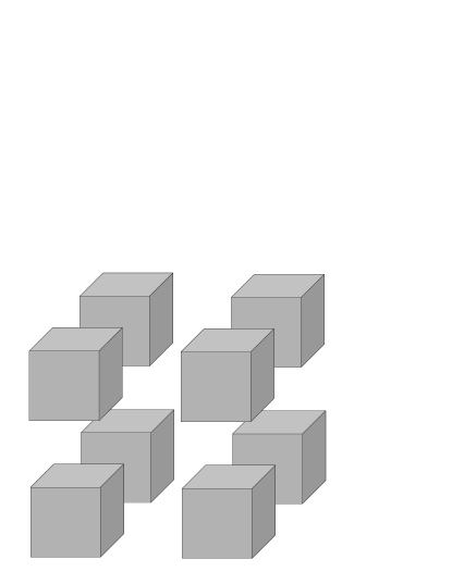
Figure 7: Phase 3 of spin 1. The bond variables have higher expectation values on the cubes shown.

Phase 4. There are four degenerate states:

$$\phi_{1}=1,~{}\phi_{2}=e^{i\alpha_{2}},~{}\phi_{3}=e^{i\alpha_{3}};$$ (32)

$$\alpha_{2}=0,\pi;~{}\alpha_{3}=0,\pi;$$ (33)

$$B_{0}=3;~{}D_{x}=D_{y}=D_{z}=2;$$ (34)

$$\epsilon_{x}=4-4(-1)^{y+z},~{}\epsilon_{y}=4-4(-1)^{z+x},$$

$$\epsilon_{z}=4-4(-1)^{x+y};$$ (35)

$$f_{x}=f_{y}=f_{z}=0.$$ (36)

This state breaks lattice symmetries as can be seen from the plaquette energies. However, because the bond variables $f_{x,y,z}$ are zero, we do not know a simple interpretation of this phase in terms of the original spins; some finer characterization than what we use here is needed to establish this state.

This concludes the discussion of the general phase diagram of the Landau theory including quadratic and quartic terms. Higher-order interactions may stabilize some other phases, but the presented states are the most natural ones. The actual lowest-energy state depends on the parameters $u,v,w$, unknown apriori. If we are to guess which of the four phases is the most likely candidate in the specific frustrated XY model, we can consider the simplest microscopic quartic potential $|\Phi|^{4}$. When expanded in terms of the continuum fields, we find $u=2$, $v=-1$, $w=-1/2$; this point is denoted by the cross in Figure 5 and lies in the Phase 1, i.e., the Haldane chains phase.

III.2.2 Analysis 2: The ground state of the XY model

Minimizing the classical energy of the hard spin XY model as described in Sec. III.1, we find that the ground state configurations coincide with the condensate wavefunctions of the phase 1 and hence the state is that of the phase 1. In particular note that each wavefunction $\Psi_{1,2,3}$ has the same length $|\Phi|$ on all sites. The XY angles of spins in this gauge in the three ground states are

$$(0,-30,-30,0,60,-90,-90,60)~{},$$ (37)

$$(0,30,30,0,-60,90,90,-60)~{},$$ (38)

$$(0,-90,90,180,0,-90,90,180)~{},$$ (39)

where the convention is that we vary position on the cube in the x direction first, then in the y direction, and then in the z.

III.2.3 Discussion and extension to anisotropic system

Some remarks are in order. First, it is useful to note that the doublet $F_{1,2}$ can be interpreted as an order parameter of the Haldane chains phase. Indeed, one can readily see that the transformation properties of $F_{1}$ and $F_{2}$ coincide with those of $(Q_{x}+Q_{y}-2Q_{z})/\sqrt{3}$ and $Q_{x}-Q_{y}$ respectively, where $Q_{m}$ is the bond variable in the direction $\hat{m}$. On the other hand, $N_{x}$ transforms as $(-1)^{x}Q_{x}$ and similarly for $N_{y}$ and $N_{z}$, so $\vec{N}$ can be viewed as an order parameter of the valence bond solids such as the columnar Phase 2 or the box Phase 3. In the columnar phase, it is suggestive to view each strong bond in Fig. 6 as representing a singlet formed by two spin-1’s, which can be also drawn as two spin-1/2 valence bonds connecting the two sites. However, we should be cautious with such interpretation, since we can only tell that the deviations of the bond variables from their mean value will have the displayed pattern. The actual state needs to be studied by constructing the corresponding spin wavefunction. For example, the Haldane phase of a spin 1 chain is stable to weak dimerization and should be viewed as a solid formed by single-strength bonds along the chains, so such distinct possibilities should be kept in mind.

Let us now assume that the system is in the Phase 1. It is also interesting to ask what happens when we stretch the lattice in one of the axis directions, say the z-direction. In this case the $R_{x}$ and $R_{y}$ rotations are no longer symmetries but the other transformations are. At the quadratic level, the translation symmetries already prohibit all terms except $B_{0}$ and $F$’s. Then from $R_{z}$ we see that only $F_{1}$ is allowed. Thus at the quadratic level one new term is allowed. In principle we should look at the new allowed terms at the quartic level, however we will assume that this quadratic term is leading but small compared to the terms that were there before we broke the symmetry.

We find that if the $F_{1}$ comes with a positive pre-factor, out of the three ground states it selects the state with chains running along the z direction whereas if it comes with a negative pre-factor it selects the two states with chains running along the x and y directions.

This has a simple interpretation in terms of spins. If the coupling in the z direction is stronger than in the other directions the state with maximum number of bonds in this directions is selected which is the state with chains running in the z-direction. In the opposite case, the states with fewest bonds in the z direction are selected which are the states with chains running in the x or y directions.

III.3 Results: Spin 3/2

III.3.1 Analysis 1: Phase transition of the XY model

We choose the gauge as shown on Figure 3 with $S=3/2$. The hopping amplitudes are

$$t_{x} = \frac{1}{\sqrt{2}}(-1)^{z}\left[1+i(-1)^{x+y}\right]~{},$$ (40)

$$t_{y} = \frac{1}{\sqrt{2}}(-1)^{z}\left[1-i(-1)^{x+y}\right]~{},$$ (41)

$$t_{z} = 1~{}.$$ (42)

The band structure has four minima and hence the space of the ground states of kinetic energy is four-dimensional. Unlike the spin 1 case where this space was three-dimensional and simple basis vectors were found corresponding to the three directions of the physical space, there is no such form in the spin 3/2 case. The four wavefunctions that give us relatively simple subsequent analysis are the following

$$\Psi_{1} = (-1)^{x}\left[\cos\beta-i(-1)^{x+y+z}\sin\beta\right]~{},$$

$$\Psi_{2} = i(-1)^{y}\left[\cos\beta+i(-1)^{x+y+z}\sin\beta\right]~{},$$

$$\Psi_{3} = \frac{1+i(-1)^{x+y}}{\sqrt{2}}\left[\cos\beta-i(-1)^{x+y+z}\sin\beta\right]~{},$$

$$\Psi_{4} = \frac{1-i(-1)^{x+y}}{\sqrt{2}}\left[\cos\beta+i(-1)^{x+y+z}\sin\beta\right]~{},$$

where

$$\cos\beta=\sqrt{\frac{\sqrt{3}+1}{2\sqrt{3}}}~{},\quad\quad\sin\beta=\sqrt{\frac{\sqrt{3}-1}{2\sqrt{3}}}~{}.$$ (43)

We again write $\Phi(R)=\sum_{i=1}^{4}\phi_{i}\Psi_{i}(R)$. The transformation properties of the slow fields $\phi_{1,2,3,4}$ are derived in the same manner as in the spin 1 case. The symmetries are

$$T_{x}: \vec{\phi}\to\tau^{3}\sigma^{0}\vec{\phi^{*}}~{},$$ (44)

$$T_{y}: \vec{\phi}\to\tau^{0}\sigma^{0}\vec{\phi^{*}}~{},$$ (45)

$$T_{z}: \vec{\phi}\to\tau^{1}\sigma^{0}\vec{\phi^{*}}~{},$$ (46)

$$R_{y}: \vec{\phi}\to\tau^{1}e^{-i\frac{\pi}{4}\tau^{2}}\sigma^{1}e^{i\frac{\pi}{3}\sigma^{2}}\vec{\phi^{*}}~{},$$ (47)

$$R_{z}: \vec{\phi}\to e^{-i\frac{\pi}{4}\tau^{3}}\sigma^{1}\vec{\phi^{*}}~{}.$$ (48)

Here $\vec{\phi}$, $\vec{\phi^{*}}$ are column vectors, and we introduced two sets of Pauli matrices: $\tau$ matrices that act on the blocs $\{1,2\}$ and $\{3,4\}$, and $\sigma$ matrices that act within each bloc ($\tau^{0}$ and $\sigma^{0}$ are the corresponding identity matrices). At the quadratic order there is one invariant term

$$V^{(2)}=m\sum_{i=1}^{4}|\phi_{i}|^{2}~{}.$$ (49)

At the quartic order there are five invariant terms. The expressions in terms of $\phi$ are rather complicated and not very illuminating, particularly since $\phi$’s depend on the choice of gauge and the basis. Instead, we will use gauge invariant bilinears of $\phi$ to which we now turn.

There are $16$ bilinears and they can be conveniently organized using tensor product of the introduced two sets of Pauli matrices, namely $\phi^{\dagger}\tau^{\mu}\sigma^{\nu}\phi$ with $\mu,\nu=0,1,2,3$. These break up into irreducible representations of the cubic lattice symmetry group. There are two one-dimensional, one two-dimensional, and four three-dimensional representations. The convenient combinations that we use are

$$B_{0} = \phi^{\dagger}\tau^{0}\sigma^{0}\phi~{},$$

$$C = \phi^{\dagger}\tau^{0}\sigma^{2}\phi~{},$$

$$F_{1} = \phi^{\dagger}\tau^{0}\sigma^{1}\phi~{},$$

$$F_{2} = \phi^{\dagger}\tau^{0}\sigma^{3}\phi~{},$$

$$\vec{D} = (D_{x},D_{y},D_{z})=\phi^{\dagger}\vec{\tau}\sigma^{2}\phi~{},$$

$$\vec{N} = (N_{x},N_{y},N_{z})=\phi^{\dagger}\vec{\tau}\sigma^{0}\phi~{},$$

$$M_{x} = \phi^{\dagger}\tau^{1}(-\frac{1}{2}\sigma^{1}-\frac{\sqrt{3}}{2}\sigma^{3})\phi~{},$$

$$M_{y} = \phi^{\dagger}\tau^{2}(-\frac{1}{2}\sigma^{1}+\frac{\sqrt{3}}{2}\sigma^{3})\phi~{},$$

$$M_{z} = \phi^{\dagger}\tau^{3}\sigma^{1}\phi~{},$$

$$K_{x} = \phi^{\dagger}\tau^{1}(\frac{\sqrt{3}}{2}\sigma^{1}-\frac{1}{2}\sigma^{3})\phi~{},$$

$$K_{y} = \phi^{\dagger}\tau^{2}(-\frac{\sqrt{3}}{2}\sigma^{1}-\frac{1}{2}\sigma^{3})\phi~{},$$

$$K_{z} = \phi^{\dagger}\tau^{3}\sigma^{3}\phi~{}.$$

The transformation properties of these bilinears are in the following table

$T_{x}$ $T_{y}$ $T_{z}$ $R_{x}$ $R_{y}$ $R_{z}$ $B_{0}$ + + + + + + $C$ $-$ $-$ $-$ + + + $F_{1}$ + + + $-\frac{1}{2}F_{1}+\frac{\sqrt{3}}{2}F_{2}$ $-\frac{1}{2}F_{1}-\frac{\sqrt{3}}{2}F_{2}$ + $F_{2}$ + + + $\frac{\sqrt{3}}{2}F_{1}+\frac{1}{2}F_{2}$ $-\frac{\sqrt{3}}{2}F_{1}+\frac{1}{2}F_{2}$ $-$ $D_{x}$ + $-$ $-$ + $D_{z}$ $D_{y}$ $D_{y}$ $-$ + $-$ $D_{z}$ + $D_{x}$ $D_{z}$ $-$ $-$ + $D_{y}$ $D_{x}$ + $N_{x}$ $-$ + + + $N_{z}$ $N_{y}$ $N_{y}$ + $-$ + $N_{z}$ + $N_{x}$ $N_{z}$ + + $-$ $N_{y}$ $N_{x}$ + $M_{x}$ $-$ + + + $M_{z}$ $M_{y}$ $M_{y}$ + $-$ + $M_{z}$ + $M_{x}$ $M_{z}$ + + $-$ $M_{y}$ $M_{x}$ + $K_{x}$ $-$ + + $-$ $-K_{z}$ $-K_{y}$ $K_{y}$ + $-$ + $-K_{z}$ $-$ $-K_{x}$ $K_{z}$ + + $-$ $-K_{y}$ $-K_{x}$ $-$


The energies and staggered curls of monopole currents in term of these bilinears are

$$\epsilon_{x} = \frac{2}{\sqrt{3}}B_{0}-2(-1)^{y+z}D_{x}$$ (50)

$$- \sqrt{2}\left[(-1)^{y}M_{y}+(-1)^{z}M_{z}\right]$$

$$+ \sqrt{\frac{2}{3}}\left[(-1)^{y}K_{y}-(-1)^{z}K_{z}\right]~{},$$

$$f_{x} = 2\sqrt{2}(F_{1}+\sqrt{3}F_{2})+\frac{8(-1)^{x}}{\sqrt{3}}N_{x}~{}.$$ (51)

The components in the other directions are obtained from these by simple rotations of the coordinates. Our general discussion following similar expressions (17) and (18) in the spin 1 case apply here as well (for ease of comparison, we are using similar labels for objects with identical transformation properties in the two cases). However, a word of warning is in order here, which will be explained in Sec. III.3.3 below. Observe, for example, that $\vec{N}$ and $\vec{M}$ have identical transformation properties and therefore should enter similarly in any expression. The absence of $M$’s in the expression for $\epsilon_{x}$ and the absence of $N$’s in the expression for $f_{x}$ is due to their different eigenvalues under an additional artificial symmetry present in the frustrated XY model, namely a charge conjugation symmetry defined later, which is also present in our bare kinetic term and thus in the above expressions. This symmetry is not physical in the original spin model and will not be used here; it is therefore important to note that the degeneracy of the four slow modes obtained from the bare kinetic term is protected at the quadratic level by the physical lattice symmetries.

There are five independent fourth order terms in $\phi$ allowed by translation and rotation symmetries:

$$I_{1} = B_{0}^{2}~{},$$ (52)

$$I_{2} = C^{2}~{},$$ (53)

$$I_{3} = N_{x}^{2}+N_{y}^{2}+N_{z}^{2}~{},$$ (54)

$$I_{4} = M_{x}^{2}+M_{y}^{2}+M_{z}^{2}~{},$$ (55)

$$I_{5} = N_{x}M_{x}+N_{y}M_{y}+N_{z}M_{z}~{}.$$ (56)

As we have said earlier, because the number of invariant terms is large, we will not attempt to draw the phase diagram of the Landau’s theory. Instead we look at the natural microscopic term

$$V^{(4)}=|\Phi|^{4}=\frac{4}{3}I_{1}+\frac{1}{3}I_{2}-\frac{1}{3}I_{3}+\frac{2}{3}I_{4}~{},$$ (57)

where the second equality is obtained after some calculation keeping only non-oscillatory terms.

This potential does not have any continuous symmetry left other than the global $U(1)$ transformation of all fields. In fact the dimensions of the subgroups of $SU(4)$ that keep the terms $I_{1},\ldots,I_{5}$ invariant are $15,7,6,0,0$ respectively. The potential (57) achieves global minimum at twelve discrete points. As an illustration, we consider the following four minima that are associated with the $z$ direction in the sense to become clear below: $(\phi_{1},\phi_{2},\phi_{3},\phi_{4})=$

$$(1,0,0,0),~{}~{}(0,1,0,0),~{}~{}(0,0,1,0),~{}~{}(0,0,0,1).$$ (58)

The four states can be related to each other by translations in the z direction and rotations about the z axis. Besides $B_{0}=1$, the only nonzero bilinears in these states are $(F_{2},N_{z},K_{z})=(1,1,1)$, $(-1,1,-1)$, $(1,-1,-1)$, and $(-1,-1,1)$ respectively.

The energies are

$$\epsilon_{x} = \frac{2}{\sqrt{3}}\mp(-1)^{z}\sqrt{\frac{2}{3}}~{},$$ (59)

$$\epsilon_{y} = \frac{2}{\sqrt{3}}\pm(-1)^{z}\sqrt{\frac{2}{3}}~{},$$ (60)

$$\epsilon_{z} = \frac{2}{\sqrt{3}}~{},$$ (61)

where the upper sign corresponds to the first and fourth minima and the lower sign to the other two.

The staggered curls of monopole currents are respectively

$$f_{x},f_{y},f_{z}=$$

$$2\sqrt{6},-2\sqrt{6},\frac{8(-1)^{z}}{\sqrt{3}}~{},$$ (62)

$$-2\sqrt{6},2\sqrt{6},\frac{8(-1)^{z}}{\sqrt{3}}~{},$$ (63)

$$2\sqrt{6},-2\sqrt{6},-\frac{8(-1)^{z}}{\sqrt{3}}~{},$$ (64)

$$-2\sqrt{6},2\sqrt{6},-\frac{8(-1)^{z}}{\sqrt{3}}~{}.$$ (65)

The staggered curls are interpreted as the strength (above some mean) of the expectation value of nearest neighbor spin-spin correlation function. The above values imply that the spins organize themselves into ladders as shown in Figure 2, obtained by drawing say the positive bonds for the first of the above minima. The four listed states correspond to the four different positions of ladders with rungs oriented along the z-axis. The other eight minima are obtained by 90 degree rotations around the x and y axes and we will not write the specific values of the variables. The ladder state is natural for $S=3/2$ system, in the picture where spin $3/2$ breaks up into three spin $1/2$’s and each of them forms a bond with some other neighboring spin $1/2$.

III.3.2 Analysis 2: The ground state of the XY model

We can use the same procedure as in the case of spin 1 to find the classical ground state of the appropriate XY model. In fact, this was already done in Ref. Diep, because this problem is the fully frustrated XY model (FFXY), which is of interest by itself, and we can use the available results. We find that the ground state configurations coincide with the condensate wavefunctions obtained above. Thus, in each of the four displayed states (58), the microscopic boson field $\Phi$ is given precisely by one of the four wavefunctions $\Psi_{1,\dots,4}$. One can see that $|\Phi|=1$ on all lattice sites, and the complex phases of $\Phi$ can be interpreted as angles of the hard-spin XY model. For example, for $\Phi=\Psi_{1}$ the angles are

$$(-\beta,\pi+\beta,\beta,\pi-\beta,\beta,\pi-\beta,-\beta,\pi+\beta)~{},$$ (66)

listed in the same order as in Eq. (39). All other ground states can be obtained by appropriate symmetry transformations. The agreement of the two analyses suggests that there is only one ordered phases in the FFXY model, which is also supported by the available Monte Carlo studies.Diep ; KimStroud

III.3.3 Remark on charge conjugation symmetry in the FFXY

It is worth to point out that the fully frustrated XY model has an additional charge conjugation symmetry. Indeed, since $\pi$ and $-\pi$ fluxes are indistinguishable, $t_{RR^{\prime}}$ and $t_{RR^{\prime}}^{*}$ are related by a gauge transformation, $t_{RR^{\prime}}=e^{i\gamma_{R}}t_{RR^{\prime}}^{*}e^{-i\gamma_{R^{\prime}}}$, and so the action remains invariant under the following unitary transformation:

$${\cal C}:\Phi_{R}\to e^{i\gamma_{R}}\Phi_{R}^{*}~{}.$$ (67)

In terms of the continuum fields, this becomes

$${\cal C}:\vec{\phi}\to\tau^{2}\sigma^{2}\vec{\phi^{*}}~{}.$$ (68)

In particular, the bilinears $N_{x,y,z}$ are odd under ${\cal C}$ while $M_{x,y,z}$ are even, so if this symmetry is included, the $I_{5}$ quartic term is not allowed (this is why this term did not appear in Eq. 57 since both the microscopic $|\Phi|^{4}$ and the bare quadratic terms in Eq. 10 have this additional symmetry). Thus, the complete field theory for the FFXY model is a $\phi^{4}$ theory with four complex fields and independent quartic terms $I_{1,\dots,4}$.

One consequence of the charge conjugation symmetry is that, for example, if we draw the $\Psi_{1}$ state using negative values of the staggered curls $f_{x,y,z}$ as opposed to using positive values which was done in Fig. 2, we would obtain another set of ladders that go perpendicularly to the ones displayed and are shifted up by one lattice spacing. To put this in other words, the $\Psi_{1}$ and $\Psi_{4}$ states that can be related by a translation in the z direction followed by a rotation around the z axis are also related by ${\cal C}$. In this sense, each of the states Eq. (58) does not define a direction in the x-y plane since the correlations in the x and y directions are related by the charge conjugation symmetry.

Tracing back to the original gauge theory formulation, this symmetry is present in the simplest model Eq. (5) for $S=3/2$ that we wrote down and the corresponding simplest “dimer model” Hamiltonian Eq. (6). Specifically, the transformation $E\to 1-E$ on the links oriented from one sublattice to the other, or equivalently $1\leftrightarrow 0$ in the dimer language, takes the model corresponding to spin $S$ to the one corresponding to spin $3-S$, while the $S=3/2$ case maps back onto itself. This symmetry is useful in the specific models, but there is no corresponding symmetry in the microscopic derivation from the spin model, and therefore it was not used in the preceding analysis.

Let us look what happens to the ground states when we add small term that breaks the charge conjugation symmetry, the $I_{5}$, to the potential. Using general arguments it is easy to check that the twelve minima will shift but not split, and the twelve-fold degeneracy remains since all are related to each other by lattice symmetries. Furthermore, each ground state stays translationally invariant along the ladders and perpendicular to the plane of ladders (otherwise, if this were not true, there would be more than twelve states). In other words, the states still have the structure of ladders. However since the charge conjugation is broken, it is no longer true that the negative bonds are of the same magnitude as the corresponding positive ones. This makes sense when interpreted in terms of spins. In the picture where spin $3/2$ breaks up into three spin $1/2$ and ladders of valence bonds are formed, the links that belong to these ladders are different from the links without bonds (which also form ladders). For example, the system is entangled along the former but not along the latter. Thus these two should not be related by any symmetry.

Explicitly, the four states in Eq. (58) become

$$(1,\delta,0,0),~{}~{}(\delta,1,0,0),~{}~{}(0,0,1,\delta),~{}~{}(0,0,\delta,1),$$ (69)

with appropriate $\delta$ obtained from minimization. There is now an additional non-zero bilinear $M_{z}$, and also both $F_{1}$ and $F_{2}$ are non-zero. The expressions for the energies and staggered curls in the x and y directions are no longer related, and we can then associate a unique x or y direction with each of the four states. These are ladders with rungs oriented in the z direction and are related to each other by the z translations and rotations.

III.3.4 Extension to anisotropic system

As in the spin 1 case, we ask what happens when we stretch the system along one axis, say the z-direction. Again, the $R_{x}$ and $R_{y}$ rotations are no longer symmetries but the translations and $R_{z}$ are. At the quadratic level, the translation symmetries already prohibit all terms except $B_{0}$ and $F$’s. Then from $R_{z}$ we see that only $F_{1}$ is allowed. Thus at the quadratic level one new term is allowed.

We find that if the $F_{1}$ comes with a positive pre-factor, out of the twelve ground states it selects four with the ladders that lie entirely in the x-y plane, whereas if it comes with a negative pre-factor it selects four states with the ladders running along the z-direction. Note that this breaking up into groups of four is a consequence of the remaining symmetries in the system.

These results have a simple physical interpretation for the spin system. If the coupling in the z direction is weaker than in the other directions, the states with fewest bonds in the z direction are selected which are the states with the ladders lying in the x-y plane. On the other hand, if the coupling in the z direction is stronger, the states with the largest number of bonds in the z direction are selected, which are the states with ladders oriented in the z direction.

IV Analysis 3: Mapping to dimers at $\lambda\gg 1/\beta\gg 1$

Here we look at the right hand corner of the phase diagram Fig. 4 in the regime with $\lambda\gg 1/\beta\gg 1$, where as we will see the system can be mapped to dimers. ZhengSachdev ; FradkinKivelson ; FradkinBook

The analysis proceeds as follows. First we gauge away the $\nabla\theta$ in Eq. (9) to obtain

$$S_{\rm dual}=\sum\frac{(\partial L)^{2}}{8\pi^{2}\beta}-\sum\lambda\cos(L+L^{0})~{},$$ (70)

Because we assume $\lambda\gg 1/\beta\gg 1$ the configurations that contribute significantly to the partition function can be written in the form $L=-L^{0}+2\pi n+\delta L$ where $n$ is an integer and $\delta L$ is small. Note that the $\lambda$ term does not depend on $n$ and the $1/\beta$ term has a gauge invariance $n\to n+\nabla m$ where $m$’s are integers on sites. The partition function can be written as a sum over the gauge equivalent classes. These classes are in one-to-one correspondence with the fluxes $j=\partial n$ which are integers on plaquettes, where $\partial n$ is the four dimensional curl $(\partial n)_{\mu\nu}=\partial_{\mu}n_{\nu}-\partial_{\nu}m_{\mu}$.

Consider first configurations with $\delta L=0$. Some configurations of $j$ minimize the action and we denote them by $j^{gs}$. As we show below, there is an extensive number of them in all our cases. The configurations with $j$ that are not $j^{gs}$ are at energy of at least $\sim 1/\beta$ higher. Now turning on $\delta L$, if we show that the typical energy of excitation in $\delta L$ around a given $j$ is much smaller then $1/\beta$ then we can neglect all configurations which are not around $j^{gs}$. We will assume that this is true and show this self-consistently below.

We define $J^{gs}=-\partial L^{0}/(2\pi)+j^{gs}$. We expand the action to the second order and drop the terms that do not depend on $J^{gs},\delta L$ to obtain

$$S\approx\sum\frac{4\pi J^{gs}\cdot(\partial\delta L)+(\partial\delta L)^{2}}{8\pi^{2}\beta}+\sum\frac{\lambda}{2}(\delta L)^{2}~{}.$$ (71)

This is just a gaussian integral. There are two quadratic terms and the first one has $1/\beta$ in front and contains two derivatives while the second has $\lambda$ in front and contains no derivatives. Since we are on a lattice the derivatives are of order one. Since $\lambda\gg\beta$, the first term can be neglected. Next we sum by parts and integrate out the $\delta L$. Before we do this however, we notice that the coupling is ferromagnetic in time direction and $L^{0}$ has zero time components and its spatial components do not depend on time. This implies that the $j^{gs}$ and $J^{gs}$ have zero time components and their spatial components do not depend on time. Thus we drop time components and time derivatives from the action and treat the $J^{gs}$ and $L^{0}$ as three-dimensional. Now we integrate out the $\delta L$ and obtain

$$S_{\rm eff}[J^{gs}] = -\frac{1}{8\pi^{2}\beta^{2}\lambda}\sum(\nabla\times J^{gs})^{2}$$ (72)

Thus, to obtain a ground state, we need to maximize the sum of the squares of curls of $J^{gs}$.

Let us check the consistency of our approach. From (71), $\delta L\sim\nabla\times J^{gs}/(\lambda\beta)$ and so energy$\sim 1/(\lambda\beta^{2})$. This needs to be much smaller then $1/\beta$ which implies $\lambda\gg 1/\beta$ which is what we assumed.

Figure 8: a) $L^{0}/(2\pi)$ where $S=1/2,1,3/2$ is the spin. The link variables switch orientations under elementary translation in the x or y direction. b) The fluxes $(\nabla\times L^{0})/(2\pi)$. This figure is similar to Fig. 3 with $2\pi$’s removed to simplify the discussion of the dimer ground states.

Now let us turn to the specific cases of spins. Since the spin 1/2 case has not been considered using this approach before, we will add it here for completeness. The gauge choice for $L^{0}$ and the fluxes $\nabla\times L^{0}/(2\pi)$ through the faces of the spatial cubes are shown on Figure 8 with $S=1/2$. It is easy to see that the set of ground states consists of all configurations with precisely one $-5/6$ and five $1/6$ fluxes $J^{gs}$ coming out of every site of one sublattice of the original spin lattice (and coming into every site on the other sublattice). $J^{gs}=-\nabla\times L^{0}/(2\pi)$ is one such configuration in the spin 1/2 case, but there are many more. Associating the $-5/6$ plaquettes with dimers on the links of the original spin lattice, the set of the ground states is thus the set of dimer configurations with one dimer coming out of every site.

Now turn to the case of spin 1. The fluxes $(\nabla\times L^{0})/(2\pi)$ are shown on Figure 8 with $S=1$. If we try $J^{gs}=-\nabla\times L^{0}/(2\pi)$, each cube contributes $1/\beta$ energy term proportional to $5(1/3)^{2}+(5/3)^{2}=10/3$. However we can do better. Using $L=-L^{0}+2\pi n$, if we pick $n=1$ on the upper link on the front face and zero elsewhere on the cube in Fig. 8, we lower the magnitude of the flux on the upper face, at the expense of increasing the flux through the front face. The energy of this cube is then $4(1/3)^{2}+2(2/3)^{2}=4/3$, which is lower. It is easy to show that this is the lowest we can achieve and that the ground state configurations have two fluxes of value $-2/3$ and four fluxes of value $1/3$ coming out of every site of one sublattice of the original spin lattice. Associating the $2/3$ links with dimers, the set of the ground states is thus the set of dimer configurations with two dimers coming out of every spin site.

Finally, in the $S=3/2$ case, it is easy to see that the ground state configurations have precisely three $-1/2$ and three $1/2$ fluxes coming out of every site of one sublattice of the original cubic lattice. Associating the $-1/2$ links with dimers, the set of the ground states is thus the set of dimer configurations with three dimers coming out of every spin site.

Thus, as claimed, in each case there is an extensive number of $J^{gs}$’s. To find the true ground state, we need to minimize (72) among these dimer configurations. It is not hard to show that for the spin $1/2$ we get columnar state, for spin $1$ the Haldane chains state of Fig. 1 and for spin $3/2$ the ladder state of Fig. 2.

Finally we note that defining $E^{gs}=S/3-J^{gs}$, the set of $E^{gs}$ is the set of electric fields on links, cf. Eq. (6), with the property that the magnitude of each is either zero or one (which can be imposed by minimizing the energy term $\sum E^{2}$); the mapping between such electric fields and dimers above is the standard one on the cubic lattice ZhengSachdev ; FradkinKivelson ; FradkinBook . The final ground state selection is obtain by maximizing $\sum(\nabla\times E)^{2}$.

V Conclusions

In this paper we looked for spin solid phases in the system of spin $1$ and $3/2$ on the cubic lattice. We wrote the spins in terms of Schwinger bosons, assumed the uniform Coulomb spin liquid phase and by process of monopole condensation transitioned into spin solid phases. Using the duality we rewrote the system in terms of monopoles coupled to a noncompact $U(1)$ gauge field, Eq. (9), and analyzed this theory in three different limits shown in Figure 4.

In the first two limits the theory becomes a frustrated XY model. For spin $1$ the frustrating flux through every plaquette is $2\pi/3$, while for spin $3/2$ it is $\pi$. In the first approach, using symmetries we wrote the Landau’s theory near the ordering transition. It is a $\phi^{4}$ theory with $\phi$ a complex vector with three components for $S=1$ and four components for $S=3/2$. At the quadratic level only the rotationally invariant mass term is allowed. At the quartic level there are three allowed terms for spin $1$ and five for spin $3/2$. For spin $1$ we draw a mean field phase diagram Figure 5. For spin $3/2$ we didn’t attempt it due to a large number of parameters. In both cases we also considered the most natural microscopic potential and found that it selects a state with parallel Haldane chains of Figure 1 for $S=1$ and a state with parallel ladders of Figure 2 for $S=3/2$. These are natural states for the spin systems to be in, in the picture where spin $1$ breaks up into two and spin $3/2$ into three spin $1/2$’s and each such spin $1/2$ forms a singlet bond with another spin $1/2$ of some neighbor.

In the second approach we looked at the classical ground states of the frustrated XY models and found that these actually describe the same phases as the most natural ones identified near the transition.

In the third approach the theory becomes a dimer model with $2S$ dimers coming out of every site. Dimer configurations with parallel lines for spin $1$ and parallel ladders for spin $3/2$ are selected, which is the same result as in the other two limits suggesting that these are indeed the most natural valence bond solids in the corresponding spin systems. It would be interesting to look for such spin solid phases in Quantum Monte Carlo studies of models on the cubic lattice.Beach ; Harada3d

It is also worth notingBergman that if we consider our quantum 3d systems at a finite temperature, we obtain simply the corresponding classical 3d dimer models, e.g., with the classical energy given by the first term in Eq. (6). Our results then provide appropriate long-wavelength (dual) description of the dimer ordering patterns transitioning out of the so-called Coulomb phase of the classical dimer models,Huse ; Hermele ; Alet stressing in particular a composite character of the naive order parameters for the valence bond solid phases. It would interesting to explore such 3d classical dimer models and their transitions further.

Appendix A Classical $U(1)$ duality with background charge

In this section we derive duality for classical compact $U(1)$ gauge theory.Peskin ; MotrunichSenthil However we will use a general notation of antisymmetric tensors, or differential forms which are fields of antisymmetric tensors. Thus the derivation will work not only for the gauge theory, whose objects are one dimensional, but for general $n$-dimensional objects. For $n=0$ this is the vortex duality of the XY model and for $n=1$ the duality of the gauge theory. The further advantage of this derivation is that the formulas are simpler and more transparent.

First we give the basic notations and properties of antisymmetric tensors. An $n$-dimensional antisymmetric tensor $\omega$ in $d$ dimensions is a collection of numbers $\omega_{\mu_{1},\mu_{2},\ldots,\mu_{n}}$, where $\mu_{v}=1,\ldots,d$, which is completely antisymmetric. A differential form $\omega(\vec{r})$ is a field of these tensors.

We define two operations. First is the exterior derivative $\partial$. The derivative of $\omega$, denoted $\partial\omega$ is the $(n+1)$-form

$$(\partial\omega)_{\mu_{1},\mu_{2},\ldots,\mu_{n+1}}=\frac{1}{n!}\sum_{p}(-1)^{p}\partial_{\mu_{p_{1}}}\omega_{\mu_{p_{2}},\ldots,\mu_{p_{n}}}$$ (73)

where the sum is over all permutations of the $n+1$ indices and $(-1)^{p}$ is $-1$ if the permutation is odd and $1$ if it is even. Thus for example for $n=1$, a vector field, $(\partial\omega)_{12}=\partial_{1}\omega_{2}-\partial_{2}\omega_{1}$ and hence this is the curl of a vector field.

The second operation that we define is the star operator that takes $n$-form to $(d-n)$-form

$$(*\omega)_{\nu_{1},\ldots,\nu_{d-n}}=\frac{1}{n!}\epsilon_{\nu_{1},\ldots,\nu_{d-n},\mu_{d-n+1},\ldots,\mu_{d}}\omega_{\mu_{d-n+1},\ldots,\mu_{d}}$$ (74)

where $\epsilon$ is the fully antisymmetric tensor in $d$ dimensions and repeated indices are summed over. For example in three dimensions for $n=2$, $(*\omega)_{1}=\frac{1}{2}(\omega_{23}-\omega_{32})$. Note that $**=(-1)^{n(d-n)}$.

A common operator is divergence which in this notation is proportional to $*\partial*$. As easily checked,

$$(\nabla\cdot\omega)_{\mu_{1},\ldots,\mu_{n-1}} \equiv \partial_{\nu}\omega_{\nu,\mu_{1},\ldots,\mu_{n-1}}$$ (75)

$$= (-1)^{(n-1)(d-n)}(*\partial*\omega)_{\mu_{1},\ldots,\mu_{n-1}}$$ (76)

For a vector field this is the standard divergence.

We will work on the lattice. The variables are defined on discrete points. We will define the coordinates of a given variable to be those of the center of the object the variable belongs to. For example the $x$ component of a one form $\omega$ in $d=3$ lies on a link pointing in $x$ direction and it is denoted by $\omega_{x}(x+1/2,y,z)$. The $\partial$ now denotes the difference operator. For example the curl of the $\omega$ is $(\partial\omega)_{xy}(x+1/2,y+1/2,z)=\omega_{y}(x+1,y+1/2,z)-\omega_{y}(x,y+1/2,z)-\omega_{x}(x+1/2,y+1,z)+\omega_{x}(x+1/2,y,z)$.

Finally we will write the integration (summation) by parts

$$\sum\omega\cdot\partial\phi=-\sum(\nabla\cdot\omega)\cdot\phi+\mbox{surface term}$$ (77)

where the dot is the sum over the component by component product of two forms of the same $n$. Note that $*\omega_{1}\cdot*\omega_{2}=\omega_{1}\cdot\omega_{2}$. Because we use periodic boundary conditions below, the surface term will be zero.

Now we are ready to turn to the duality. Let $a$ be an $n$-form in $d$ dimensions where its variables are defined on the unit circle. The action is

$$S=-\beta\sum\cos(\partial a)-i\sum\eta\cdot a$$ (78)

In the first term one takes every component at every point, takes cosine of it and sums. In the second term the $n$-form $\eta$ denotes the background charge. For the action considered in this paper, the first term is the $S_{a}$ and the second term the $S_{B}$ in (5), while the $\eta$ is the four dimensional vector with the time component being $\pm 2S$ and the other components being zero.

The duality proceeds by the following steps.

$$Z = \int_{-\pi}^{\pi}Dae^{\beta\sum\cos(\partial a)+i\sum\eta\cdot a}$$ (79)

$$\approx \int_{-\pi}^{\pi}Da\sum_{p}e^{-\frac{\beta}{2}\sum(\partial a-2\pi p)^{2}+i\sum\eta\cdot a}$$

$$= \int_{-\infty}^{\infty}Da\sum_{q^{\prime}}e^{-\frac{\beta}{2}\sum(\partial a-2\pi\partial^{-1}q^{\prime})^{2}+i\sum\eta\cdot a}$$

$$= \int_{-\infty}^{\infty}Da\sum_{q^{\prime}}\int_{-\infty}^{\infty}DJ$$

$$\times e^{-\sum\frac{J^{2}}{2\beta}+i\sum J\cdot(\partial a-2\pi\partial^{-1}q^{\prime})+i\sum\eta\cdot a}$$

$$= \sum_{q^{\prime}}\int_{-\infty}^{\infty}DJe^{-\sum\frac{J^{2}}{2\beta}-i2\pi\sum J\cdot\partial^{-1}q^{\prime}}$$

$$\times\Delta(\nabla\cdot J-\eta)$$

All numerical factors are dropped throughout, while the sign “$\approx$” is used when an approximation is being made that does not change the qualitative aspects.

In the second line we use the Villain form of the cosine. In the third line we have written the field $p=\partial\alpha+\partial^{-1}q^{\prime}$ as a curl of $\alpha$ plus a field of a particular monopole current configuration $q^{\prime}$, $\partial^{-1}q^{\prime}$. The $\partial^{-1}$ denotes a particular configuration of $p$ that gives the monopole currents - that satisfies $q^{\prime}=\partial p$. Then we shifted $a\to a-\alpha$. The summation over $\alpha$ extends the integration of $a$ over the whole real line. The prime on $q^{\prime}$ denotes that fact that we are summing over fields for which $\partial q^{\prime}=0$.

The third line can be obtained from the fourth one by completing the square, shifting $J$ and integrating it out.

In the fifth line, the $\Delta$ denotes that the operator inside of it is zero. This line is obtained from the fourth one by integrating (summing) by parts and integrating out the $a$.

Next, as shown explicitly below, in our case there are fields $J_{0}$ and $L_{0}$ such that

$$\eta = \nabla\cdot J_{0}$$ (80)

$$J_{0} = (*P\partial L_{0})/2\pi$$ (81)

$$\partial J_{0} = 0$$ (82)

The $P$ shifts a real number by a multiple of $2\pi$ so that the result is in the interval $(-\pi,\pi]$.

Using (80) in (79) we see $\partial*(J-J_{0})=0$ and hence we can write

$$J=J_{0}+(*\partial L)/2\pi$$ (83)

for some field $L$. To substitute this into (79) we notice the following

$$J^{2}=J_{0}^{2}+(*\partial L/2\pi)^{2}+2J_{0}\cdot*\partial L/2\pi\simeq J_{0}^{2}+(*\partial L/2\pi)^{2}.$$

The $\simeq$ denotes that these expressions are equal under integration, which follows from Eq. (82). Also

$$\partial^{-1}q^{\prime}\cdot*\partial L \simeq -*\partial\partial^{-1}q^{\prime}\cdot L=-*q^{\prime}\cdot L\equiv-Q^{\prime}\cdot L,$$

$$e^{i\partial^{-1}q^{\prime}\cdot*P\partial L_{0}} = e^{i\partial^{-1}q^{\prime}\cdot*\partial L_{0}}\simeq e^{-iQ^{\prime}\cdot L_{0}},$$

where $Q^{\prime}\equiv*q^{\prime}$, and we have dropped inconsequential $\pm$ signs; in the last line, the $P$ can be removed because the resulting expression, which is in the exponent, differs from the original one by a multiple of $2\pi$.

With this we can proceed to complete the duality

$$Z \approx \sum_{Q^{\prime}}\int_{-\infty}^{\infty}DLe^{-\sum\frac{(\partial L)^{2}}{8\pi^{2}\beta}+i\sum Q^{\prime}\cdot(L+L_{0})}$$ (84)

$$= \sum_{Q}\int_{-\pi}^{\pi}D\theta\int DLe^{-\sum\frac{(\partial L)^{2}}{8\pi^{2}\beta}+i\sum Q\cdot(L+L_{0}-\partial\theta)}$$

$$\approx \sum_{p}\int_{-\pi}^{\pi}D\theta\int DLe^{-\sum\frac{(\partial L)^{2}}{8\pi^{2}\beta}-\frac{\lambda}{2}(L+L_{0}-\partial\theta-2\pi p)^{2}}$$

$$\approx \int_{-\pi}^{\pi}D\theta\int DLe^{-\sum\frac{(\partial L)^{2}}{8\pi^{2}\beta}-\lambda\cos(L+L_{0}-\partial\theta)}$$

In the first line the summation over $Q^{\prime}$ is over integer fields $Q^{\prime}$ with zero divergence $\nabla\cdot Q^{\prime}=0$ - currents. In the second line we introduced $\theta$ that imposes this constraint as a Lagrange multiplier and summed by parts. In the third line we added a small term $\sum Q^{2}/2\lambda$ and assumed that it is not going to change the basic behavior of the system. Then we summed out $Q$, which introduced integer $p$ because $Q$ is an integer (this is the Poisson summation formula). The second term is the Villain form of cosine. In the last line we approximated it by cosine.

To complete it remains to find $J_{0}$ and $L_{0}$. The $\eta$ has values $\eta_{\tau}(x,y,z,\tau+1/2)=(-1)^{x+y+z}2S$ and zero for other components. As easily checked

$$(J_{0})_{\tau x}(x+1/2,y,z,\tau+1/2)=\frac{2S}{6}(-1)^{x+y+z}$$ (85)

and similarly for $y$ and $z$ with other components (other then the ones obtained by permutation of indices) being zero. This gives the right $\eta$ and satisfies $\partial J_{0}=0$. The $L_{0}$ can be chosen as on the Fig. 3.

In the final expression (84) the $L$ is $1$-form and hence a gauge field. The $\theta$ is $0$-form - a number on a circle - a matter field. Thus we obtained a noncompact $U(1)$ gauge theory coupled to scalar fields of monopoles with frustrated hopping.

References

- (1) S. Taniguchi et al., J. Phys. Soc. Jpn. 64, 2758 (1995);
- (2) D. S. Chow, P. Wzietek, D. Fogliatti, B. Alavi, D. J. Tantillo, C. A. Merlic, and S. E. Brown, Phys. Rev. Lett. 81, 3984 (1998).
- (3) H. Kageyama, K. Yoshimura, R. Stern, N.V. Mushnikov, K. Onizuka, M. Kato, K. Kosuge, C.P. Slichter, T. Goto, and Y. Ueda, Phys. Rev. Lett. 82, 3168 (1999); H. Kageyama, M. Nishi, N. Aso, K. Onizuka, T. Yosihama, K. Nukui, K. Kodama, K. Kakurai, and Y. Ueda, Phys. Rev. Lett. 84, 5876 (2000);
- (4) A. W. Sandvik, S. Daul, R. R. P. Singh, and D. J. Scalapino, Phys. Rev. Lett. 89, 247201 (2002).
- (5) K. S. D. Beach and A. W. Sandvik, cond-mat/0612126.
- (6) K. Harada, N. Kawashima, and M. Troyer, J. Phys. Soc. Jpn 76, 013703 (2007).
- (7) A. Banerjee, S. V. Isakov, K. Damle and Y. B. Kim, cond-mat/0702029.
- (8) K. Harada and N. Kawashima, Phys. Rev. B 65, 052403 (2002).
- (9) D. P. Arovas and A. Auerbach, Phys. Rev. Lett. 61, 617 (1988); Phys. Rev. B 38, 316 (1988).
- (10) N. Read and S. Sachdev, Phys. Rev. Lett. 62, 1694 (1989); Phys. Rev. B 42, 4568 (1990).
- (11) F. D. M. Haldane, Phys. Rev. Lett. 61, 1029 (1988).
- (12) O. I. Motrunich and T. Senthil, Phys. Rev. B 71, 125102 (2005)
- (13) J.-S. Bernier, Y.-J. Kao, and Y. B. Kim, Phys. Rev. B 71, 184406 (2005).
- (14) D. L. Bergman, G. A. Fiete and L. Balents, Phys. Rev. B 73, 134402 (2006)
- (15) S. Sachdev and R. Jalabert, Mod. Phys. Lett. B 4, 1043 (1990).
- (16) S. Sachdev and K. Park, Ann. Phys. (N.Y.) 298, 58 (2002).
- (17) W. Zheng and S. Sachdev, Phys. Rev. B 40, 2704 (1989).
- (18) E. Fradkin and S. Kivelson, Mod. Phys. Lett. B 4, 225 (1990).
- (19) E. Fradkin, Field Theories of Condensed Matter Systems, Westview Press, 1991
- (20) H. T. Diep, A. Ghazali, and P. Lallemand, J. Phys. C 18, 5881 (1985).
- (21) K. Kim and D. Stroud, Phys. Rev. B 73, 224504 (2006).
- (22) D. A. Huse, W. Krauth, R. Moessner, and S. L. Sondhi, Phys. Rev. Lett. 91, 167004 (2003).
- (23) M. Hermele, M. P. A. Fisher, and L. Balents, Phys. Rev. B 69, 064404 (2004).
- (24) F. Alet, G. Misguich, V. Pasquier, R. Moessner, and J. L. Jacobsen, Phys. Rev. Lett. 97, 030403 (2006).
- (25) M. Peskin, Ann. Phys. (NY) 113, 122 (1978); R. Savit, Rev. Mod. Phys. 52, 453 (1980).