Photons as quasi-charged particles

Abstract

The Schrödinger motion of a charged quantum particle in an electromagnetic potential can be simulated by the paraxial dynamics of photons propagating through a spatially inhomogeneous medium. The inhomogeneity induces geometric effects that generate an artificial vector potential to which signal photons are coupled. This phenomenon can be implemented with slow light propagating through an a gas of double-$\Lambda$ atoms in an electromagnetically-induced transparency setting with spatially varied control fields. It can lead to a reduced dispersion of signal photons and a topological phase shift of Aharonov-Bohm type.

Introduction.— It is known since the ground-breaking work of Berry on geometric phases berry:1984 that artificial gauge potentials can be induced if the spatial dynamics of a system that obeys a wave equation is confined in a certain way. For instance, if the internal Hamiltonian of neutral atoms contains an energy barrier but the spin eigenstates are spatially varying, gauge field dynamics can be induced STIRAP . In the limit of ray optics, moving atomic ensembles could simulate the propagation of light around a black hole or generate topological phase factors of the Aharonov-Bohm type PRA60:4301 , and inhomogeneous dielectric media could generally exhibit geometric effects such as an optical spin-Hall effect and the optical Magnus force Magnus .

In this paper, we propose to use electromagnetically induced transparency (EIT) to generate an artificial vector potential for the paraxial dynamics of signal photons that simulates quantum dynamics of charged particles in a static electromagnetic field. Not only the ray of light but also its mode structure is affected, resulting in a paraxial wave equation that is equivalent to the Schrödinger equation for charged particles. Furthermore, the form of the artificial vector potential can be easily controlled through spatial variations in the control fields. We suggest configurations that generate homogeneous quasi-electric and magnetic fields as well as a vector potential of Aharonov-Bohm type.

Although the treatment in this paper is based on EIT, the effect presented here is more general: it will occur in any medium that supports a set of discrete eigenmodes for a propagating signal fields with different indices of refraction. If the parameters governing these eigenmodes vary in space, the signal modes will adiabatically follow, acquiring geometric phases that affect their paraxial dynamics.

Review of EIT with multi-$\Lambda$ atoms.— The effect takes place in an atomic multi-$\Lambda$ system, in which two ground states are coupled to $Q$ excited states by $Q$ pairs of control ($\Omega_{q}$) and signal ($\hat{a}_{q}$) fields (Fig. 1). An experimentally relevant example of such system is the fundamental D1 transition in atomic rubidium, where both the ground and excited levels are split into two hyperfine sublevels vewinger . We assume that the detunings are small so each signal field $\hat{a}_{q}$ interacts only with the respective transition $\left|B\right\rangle\leftrightarrow\left|A_{q}\right\rangle$ with the associated atomic operator $\hat{\sigma}_{B,A_{q}}$ and vacuum Rabi frequency $g_{q}$. In this case, the paraxial wave equation for each signal mode can be cast into the form

$$\Bigl{(}\frac{\partial}{\partial t}+c\frac{\partial}{\partial z}-\frac{ic}{2k}\Delta_{\perp}\Bigr{)}\hat{a}_{q}=iNg_{q}\hat{\sigma}_{B,A_{q}}\;,$$ (1)

where the wave propagates along the $z$ axis, $\Delta_{\perp}=\partial^{2}_{x}+\partial^{2}_{y}$, $N$ is the number of atoms and $k$ is the wavevector which we assume approximately independent of $q$. In Ref. appel:013804 we have constructed a unitary transformation

$$\hat{a}_{q}=\sum_{s=1}^{Q}W_{qs}\,\hat{b}_{s}$$ (2)

that maps the original field modes $a_{q}$ to a new set of modes $\hat{b}_{q}$, such that one and only one of the new modes,

$$\hat{b}_{Q}=\sum_{q=1}^{Q}R_{q}^{*}\hat{a}_{q},$$ (3)

(where $R_{q}\equiv\Omega_{q}/(g_{q}\Omega_{\perp})$ and $\Omega_{\bot}\equiv\sqrt{\sum_{q=1}^{Q}|\Omega_{q}/g_{q}|^{2}}$ depend on the control fields) couples only to an atomic dark state and experiences EIT appel:013804 ; Liu06 ; Moiseev . All other superpositions of field modes are absorbed. This transformation is given explicitly by $W_{qq^{\prime}}=\gamma w_{q}w_{q^{\prime}}^{*}-\delta_{qq^{\prime}}$, with $\gamma=R_{Q}+1$ and $w_{q}=\gamma^{-1}(\delta_{Qq}+R_{q})$.

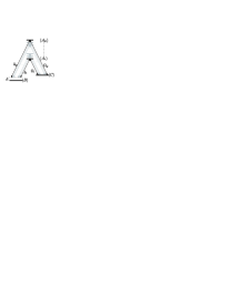
Figure 1: Multi $\Lambda$-system: $Q$ excited states $\left|A_{q}\right\rangle$ are each coupled by a classical control field $\Omega_{q}$ to the ground state $\left|C\right\rangle$ and by a quantized field $\hat{a}_{q}$ with detuning $\delta$ to state $\left|B\right\rangle$.

The EIT mode $\hat{b}_{Q}$ interacts with the multi-$\Lambda$ atoms in the same fashion as does the signal field in a regular 3-level system. While propagating through the EIT medium, it gives rise to a dark-state polariton associated with zero interaction energy fleischauer . All other modes couple to atomic states whose energy levels are Stark-shifted by the interaction with either the pump field or the other signal modes $\hat{b}_{q}$ ($q\neq Q$). The resulting energy gap guarantees that, if the amplitudes and phases of the control fields are slowly changed, the composition of the dark-state polariton, and hence the EIT mode $\hat{b}_{Q}$, will adiabatically follow. It has been proposed appel:013804 and experimentally demonstrated vewinger that a variation in time of the control fields can therefore be used to adiabatically transfer optical states between signal modes. In this paper, we focus on spatial propagation of the EIT mode under control fields that are constant in time, but varied in space.

Derivation of the gauge potential.— We proceed by expressing Eq. (1) in terms of the new signal modes $\hat{b}_{q}$. Employing the vector notation $\vec{a}=\{\hat{a}_{1},\cdots,\hat{a}_{Q}\}$ and $\vec{\sigma}_{B,A}=\{g_{1}\hat{\sigma}_{B,A_{1}},\cdots,g_{Q}\hat{\sigma}_{B,A_{Q}}\}$ we get

$$\Bigl{(}\frac{\partial}{\partial t}+c\frac{\partial}{\partial z}-\frac{ic}{2k}\Delta_{\perp}\Bigr{)}\tensor{W}\vec{\hat{b}}=iN\vec{\sigma}_{B,A}.$$ (4)

Throughout the paper, the double arrow denotes a $Q\times Q$ matrix. Because $\tensor{W}$ depends on space and time, the differential operators have to be applied to both $\tensor{W}$ and $\vec{\hat{b}}$. As a result, transformation (2) brings about additional terms into the equation of motion, that can be written in form of a minimal coupling scheme by introducing the Hermitian gauge field

$$\tensor{A}_{i}\equiv i\tensor{W}^{\dagger}\partial_{i}\tensor{W},$$ (5)

where $i=t,x,y,z$. We multiply both sides of Eq. (4) by $\tensor{W}^{\dagger}$ and exploit the unitarity of $\tensor{W}$ to show that $\partial_{i}\tensor{W}^{\dagger}=-\tensor{W}^{\dagger}(\partial_{i}\tensor{W})\tensor{W}^{\dagger}$ from which it follows that $-\tensor{W}^{\dagger}\partial_{i}^{2}\tensor{W}=\tensor{A}_{i}^{2}+i\partial_{i}\tensor{A}_{i}$. The dynamic equation for the $\hat{b}$ modes can then be written as

$$\left(i\partial_{t}+\tensor{A}_{t}\right)\vec{\hat{b}} = -\Big{(}ic\partial_{z}+c\tensor{A}_{z}\Big{)}\vec{\hat{b}}$$

$$+\frac{c}{2k}(-i\nabla_{\perp}-\tensor{A}_{\perp})^{2}\vec{\hat{b}}-\tensor{W}^{\dagger}N\vec{\sigma}_{BA}$$

with $\nabla_{\perp}=(\partial_{x},\partial_{y})$. This equation has the structure of a 2+2 dimensional field theory with minimal coupling.

Under the assumption that the control fields do not depend on $t$ and $z$ we can make a temporal Fourier transformation of the slowly varying amplitudes, which results in the paraxial wave equation

$$i\partial_{z}\vec{\hat{b}}(\delta) = \left(-\frac{\delta}{c}+\frac{1}{2k}(-i\nabla_{\perp}-\tensor{A}_{\perp})^{2}\right)\vec{\hat{b}}(\delta)$$ (7)

$$-\tensor{W}^{\dagger}\frac{N}{c}\vec{\sigma}_{BA}(\delta).$$

The gauge potential is given explicitly by

$$\tensor{A}_{\perp}=i\sum_{q=1}^{Q}R_{q}^{*}(\nabla_{\perp}R_{q})\vec{w}\vec{w}^{\dagger}-i\gamma(\nabla_{\perp}\vec{w})\vec{w}^{\dagger}+i\gamma^{*}\vec{w}\nabla_{\perp}\vec{w}^{\dagger}\;.$$ (8)

The full matrix $\tensor{A}_{\perp}$ is a pure gauge: it has emerged solely as a consequence of the unitary transformation (2), which reflects our choice to describe the system in terms of the new modes $\hat{b}_{q}$ rather than the original modes $\hat{a}_{q}$. However, this choice is motivated by the fact that the EIT mode $\hat{b}_{Q}$ is the only mode that is not absorbed. Absorption of other modes $\hat{b}_{q}$ (with $q\neq Q$) means that the index of refraction for these modes has a significant imaginary part. This separates the EIT mode $\hat{b}_{Q}$ from other $b$-modes and ensures that it will adiabatically follow variations of the control fields. Therefore, when analyzing the evolution of $\hat{b}_{Q}$, we can neglect the off-diagonal terms in the matrix $(-i\nabla_{\perp}-\tensor{A}_{\perp})^{2}$ in Eq. (7) and write

$$i\partial_{z}\hat{b}_{Q}(\delta) = -(\tensor{W}^{\dagger}\frac{N}{c}\vec{\sigma}_{BA})_{Q}(\delta)-\frac{\delta}{c}\hat{b}_{Q}(\delta)$$

$$+\frac{1}{2k}(-i\nabla_{\perp}-A_{\perp})_{Qq}(-i\nabla_{\perp}-A_{\perp})_{qQ}\hat{b}_{Q}(\delta).$$

This equation does not include the whole matrix $\tensor{A}_{\perp}$. Consequently, this potential no longer acts like a pure gauge but attains physical significance in determining the spatial dynamics of the EIT mode.

The first term on the right-hand side of Eq. (Photons as quasi-charged particles), responsible for the interaction of the light field with the EIT medium, takes the same form as the susceptibility of EIT in a single $\Lambda$-system. Neglecting decoherence, we can write it as appel:013804 $(\tensor{W}^{\dagger}\frac{N}{c}\vec{\sigma}_{BA})_{Q}(\delta)=\frac{\delta}{v_{\text{EIT}}}\hat{b}_{Q}$, with the EIT group velocity $v_{\text{EIT}}=c\Omega^{2}/(Ng^{2})$. Note that $v_{\text{EIT}}$ depends on the spatial position because $\Omega$ does. This transforms Eq. (Photons as quasi-charged particles) to

$$i\partial_{z}\hat{b}_{Q}=\left(\frac{1}{2k}(-i\nabla_{\perp}-A_{QQ})^{2}-\frac{\delta}{v_{\text{EIT}}}+\frac{\Phi}{2k}\right)\hat{b}_{Q}$$ (10)

with

$$A_{QQ} = i\sum_{q=1}^{Q}R_{q}^{*}\nabla_{\perp}R_{q}=-\sum_{q=1}^{Q}|R_{q}|^{2}\nabla_{\perp}\text{Arg}(R_{q}),$$

$$\Phi \equiv \sum_{q=1}^{Q-1}|(A_{\perp})_{Qq}|^{2}=-A_{QQ}^{2}+\sum_{q=1}^{Q}|\nabla_{\perp}R_{q}|^{2}$$ (11)

being, respectively, the “quasi-vector” and “quasi-scalar” potentials.

We see that the paraxial spatial evolution of the EIT signal mode is governed by the equation that is identical (up to coefficients) to the Schrödinger equation of a charged particle in an electromagnetic field. This is the main result of this work. By arranging the control field in a certain configuration, one can control the spatial propagation of the signal mode through the EIT medium.

Some steering of the EIT mode is possible even in a single-$\Lambda$ system by affecting the term ${\delta}/v_{\text{EIT}}$ in Eq. (10), which results in nonuniform refraction for this mode waveguiding ; SternGerlachEIT . The action of quasi-gauge fields (11) is fundamentally different: deflection of the signal field occurs not due to refraction (the refraction index on resonance is 1), but due to adiabatic following.

The case of two control fields: homogeneous electric and magnetic quasi-fields.— Of particular practical importance is the simplest non-trivial case with $Q=2$. We parametrize the control fields by writing $R_{1,2}=\sqrt{1/2\pm R}\,e^{i(\phi\pm\theta)}$. The corresponding Rabi frequencies are then $\Omega_{i}=h(x,y)\,g_{i}R_{i}$, with $h(x,y)$ being an arbitrary common prefactor. This parametrization yields the gauge potentials

$$A_{QQ} = -\nabla_{\perp}\phi-2R\nabla_{\perp}\theta;$$ (12)

$$\Phi = \frac{(\nabla_{\perp}R)^{2}}{1-4R^{2}}+(\nabla_{\perp}\theta)^{2}(1-4R^{2}).$$

Similarly to usual electrodynamics we can use a gauge transformation GaugeFootnote , $A_{QQ}^{\prime}=A_{QQ}+\nabla_{\perp}f$, to eliminate the term $\nabla_{\perp}\phi$ from Eq. (12). The common phase $\phi$ of the control fields therefore does not contribute and can be set to zero.

A simple way to generate a term that corresponds to a one-dimensional scalar potential $V(x)$ for a Schrödinger particle is to choose $R=0$ and $\theta=\int_{0}^{x}\text{d}x^{\prime}\;\sqrt{2kV(x^{\prime})}$ This choice of control fields leads to $A_{QQ}=0$ and $\Phi=2kV(x)$.

For the special case of a constant electric quasi-field along the $x$ axis, $V(x)=-Fx$ and subsequently

$$\theta=-\sqrt{4kF|x|^{3}/3},$$ (13)

where $x<0$ is assumed for the region of interest. A resonant ($\delta=0$) Gaussian solution to Eq. (10) is displayed in Fig. 2(a). The center of the Gaussian beam is shifted by an amount $x_{\text{ctr}}=Fz^{2}/{2k}$, which is equivalent to the motion of a charged particle in a constant electric field.

The control field phase profile (13) can be implemented using, for example, a phase plate. The assumption that the control fields do not depend on $z$ implies that the Fresnel number for these fields must be above 1, i.e. that the characteristic transverse distance over which these fields significantly change must be larger than $\sim\sqrt{\lambda L}$, where $L$ is the EIT cell length. This imposes a limitation on the magnitude of the electric quasi-field: from Eq. (13) we find $F\lesssim\lambda^{-1/2}L^{-3/2}$ and thus $x_{\text{ctr}}\lesssim\sqrt{L/\lambda}$. Assuming that the signal field also has a Fresnel number of at least 1, and thus satisfies $2z_{R}\gtrsim L$ (with Rayleigh length $z_{R}=kw^{2}/2$, $w$ being the signal beam width at the cell entrance), we find that in a realistic experiment, the maximum possible signal beam displacement due to the quasi-electric field is on the order of the signal beam width $w$.

To generate a homogeneous magnetic quasi-field along the z-axis the quantity $B=\nabla\times A_{QQ}=2\nabla_{\perp}\theta\times\nabla_{\perp}R$ should be constant. However, it seems difficult to simultaneously achieve a vanishing electric quasi-field ${\bf E}=-\nabla_{\perp}\Phi$. A choice that minimizes the electric quasi-field around the origin is given by $\theta=\sqrt{B/2}\,x$ and $R=\sqrt{B/2}\,y$. The quasi-potentials then become $A_{QQ}=-B\,y\,{\bf e}_{x}$, which corresponds to the Landau gauge in standard electrodynamics, and $\Phi=B+2B^{3}y^{4}+O(y^{6})$. If $\Phi$ is neglected, a Gaussian solution to the paraxial wave equation is given by

$$b_{Q} = \mathcal{N}\csc u(z)\exp\big{[}i\big{(}{\textstyle\frac{B}{4}}\cot u(z)\Delta{\bf x}^{2}+\Delta{\bf x}\cdot{\bf p}_{c}$$ (14)

$$-{\textstyle\frac{B}{2}}\Delta x\Delta y-{\textstyle\frac{1}{2B}}{p_{c,x}p_{c,y}}+{\textstyle\frac{1}{2}}y_{c}p_{c,y}\big{)}\big{]}$$

where we have set $\Delta{\bf x}\equiv(x-x_{c},y-y_{c})$, $u(z)\equiv Bz/(2k)-i\tanh^{-1}(2\eta)$ and $\eta\equiv Bw^{2}/4$. Here ${\bf x}_{c}={\bf x}_{0}+(k/B)({\bf x}^{\prime}_{0}\sin(Bz/k)+\tilde{{\bf x}}^{\prime}_{0}(1-\cos(Bz/k))$ denotes the classical spiral trajectory of a charged particle in a magnetic field, with ${\bf x}_{c}^{\prime}=d{\bf x}_{c}/dz$, initial position ${\bf x}_{0}$ and initial velocity ${\bf x}^{\prime}_{0}$. For convenience we also have defined $\tilde{{\bf x}}^{\prime}_{0}=(y^{\prime}_{0},-x^{\prime}_{0})$ and the classical canonical momentum ${\bf p}_{c}$. We remark that $p_{c,x}$ is a constant of motion. The evolution of the signal mode is displayed in Fig. 2(b).

A surprising feature of solution (14) is that the diffractive divergence of the signal beam is reduced: the width squared of the Gaussian,

$$\frac{2}{\text{Re}(iB\cot u)}=\frac{w^{2}}{8\eta^{2}}\left(1+4\eta^{2}-(1-4\eta^{2})\cos(\frac{Bz}{k})\right)\,,$$ (15)

varies periodically with $z$ instead of monotonically increasing. This effect is known for electron wavepackets takagi:JJAP2001 and can be understood as a consequence of the circular motion of particles in a magnetic field: instead of dispersing, two-dimensional particles in a magnetic field will simply move on circles of different size (depending on their velocity), but with the same angular velocity. The particle cloud will therefore not spread but “breathe”.

It remains to show that non-adiabatic coupling to other modes can be suppressed for realistic experimental parameters. This is the case if the strength of the gauge field terms coupling $b_{Q}$ to other modes, which for the quasi-magnetic field are of the order $B/(2k)$, are much smaller than the difference in the respective linear susceptibilities $\chi_{1}$. For the EIT mode $b_{Q}$, $\chi_{1}=\delta/v_{\text{EIT}}$ with $v_{\text{EIT}}$ defined above Eq. (10); for the other modes it can be approximated by the susceptibility of a two-level medium, $\chi_{1}=-4Ng^{2}(\delta-i\gamma/2)/(c\gamma^{2})$. Evaluating this relation at resonance leads to the condition $\eta\ll(kw)^{2}n3\pi/2$, with $n\equiv N/(Vk^{3})$ being the number of atoms in the volume $k^{-3}$, which can easily be fulfilled in an experiment.

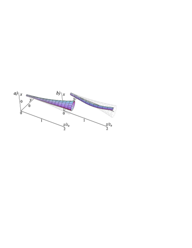
Figure 2: Paraxial propagation of a signal beam over twice the Rayleigh length in the presence (solid) and absence (grey) of a constant (a) electric field along the $x$ axis and (b) magnetic field along $z$. The dashed line represents the center of the grey beam. The effect of the fields is somewhat exaggerated.

Aharonov-Bohm potential for photons.— One of the most intriguing phenomena of charged quantum particles in electromagnetic fields is the Aharonov-Bohm (AB) effect aharonov59 . Its two astonishing features are (i) a phase shift induced by the vector potential in a region in which electric and magnetic fields are absent, and (ii) its topological nature: the phase shift does not depend on the particle trajectory as long as it encloses a magnetic flux. Because (unlike genuine electromagnetism) the potential (5) is a differential function of the control fields, it is impossible to simulate feature (i) with quasi-charged photons. However, we will show here that a mathematically equivalent topological phase shift does exist for the optical case.

To generate an AB potential for photons we propose to use two counter-rotating Laguerre-Gaussian control fields, i.e., fields that possess an orbital angular momentum. If these control fields are spatially wider than the signal fields, the corresponding Rabi frequencies can be approximated in cylindrical coordinates $(r,\varphi)$ by $\Omega_{1}=g_{1}s_{1}re^{i\varphi}$ and $\Omega_{2}=g_{2}s_{2}re^{-i\varphi}$. The gauge potentials (12) then become $A_{QQ}=-2R/r\;\vec{e}_{\varphi}$ and $\Phi=(1-4R^{2})/r^{2}$, with $R=\frac{1}{2}(|s_{1}|^{2}-|s_{2}|^{2})/(|s_{1}|^{2}+|s_{2}|^{2})$. The potential $A_{QQ}$ corresponds exactly to an Aharonov-Bohm potential for charged particles as it is created by a solenoid.

Solutions of the paraxial wave equation (10) can be found in cylindrical coordinates by expanding the field mode as $b_{Q}=r^{-1/2}\sum_{m\in\text{Z Z}}B_{m}(z,r)\exp(im\varphi)$. Because of $\Omega\sim r$, the EIT group velocity can be written as $v_{\text{EIT}}=\tilde{v}\,r^{2}$ with $\tilde{v}\equiv c\sqrt{|s_{1}|^{2}+|s_{2}|^{2}}/N$. Exact solutions are given by Bessel functions,

$$B_{m}=e^{-i\kappa^{2}z/(2k)}\left(\alpha_{m}\sqrt{\kappa r}J_{\nu}(\kappa r)+\beta_{m}\sqrt{\kappa r}Y_{\nu}(\kappa r)\right)\;,$$ (16)

with $\nu=\sqrt{1+m^{2}+4Rm-2k\tilde{v}\delta}$. For monochromatic signal fields this corresponds to a rotation of the transverse mode structure. For $R=\pm 1/2$ the potential transfers a unit amount of angular momentum to the signal light, but generally the amount can vary continuously between $-\hbar$ and $\hbar$. Signal photons in the EIT mode therefore form a two-dimensional bosonic quantum system in an Aharonov-Bohm potential.

Conclusion.— We showed that EIT in a multi-$\Lambda$ system can be used to generate a variety of geometric effects on propagating signal pulses that mimic the behavior of a charged particle in an electromagnetic field. We found specific arrangements of two spatially inhomogeneous pump fields in a double-$\Lambda$ system which generate quasi-gauge potentials which correspond to constant electric and magnetic fields. Furthermore topological effects like the Aharonov-Bohm phase shift can be induced. The latter is significantly different from the proposal of Ref. PRA60:4301 in that it is based on spatially inhomogeneous pump fields rather than the Doppler effect in moving media.

This paper investigated EIT in systems with two ground levels. In such a system, there is only one EIT mode, which results in an Abelian U(1) gauge theory, making the physics analogous to electromagnetism. By extending to multiple ground levels, it may be possible to obtain multiple EIT modes and model non-Abelian gauge potentials. This will be explored in a future publication.

- (1) M. V. Berry, Proc. R. Soc. Lond. A 392, 45 (1984).
- (2) R. Dum and M. Olshanii, Phys. Rev. Lett. 76, 1788 (1996); J. Ruseckas et al., Phys. Rev. Lett. 95, 010404 (2005); K. Osterloh et al., Phys. Rev. Lett. 95, 010403 (2005).
- (3) U. Leonhardt and P. Piwnicki, Phys. Rev. A 60, 4301 (1999).
- (4) S. Murakami, N. Nagaosa, and S.-C. Zhang, Science 301, 1348 (2003); M. Onoda, S. Murakami, and N. Nagaosa, Phys. Rev. E 74, 066610 (2006); K. Y. Bliokh and Y. P. Bliokh, Phys. Rev. Lett. 96, 073903 (2006); K. Bliokh, Phys. Rev. Lett. 97, 043901 (2006); C. Duval, Z. Horvath, and P. Horvathy, J.Geom.Phys. 57, 925 (2007); C. Duval, Z. Horvathy, and P. A. Horvathy, Phys. Rev. D 74, 021701 (2006); S. Raghu and F. D. M. Haldane, cond-mat/0602501.
- (5) F. Vewinger et al., quant-ph/0611181.
- (6) J. Appel, K.-P. Marzlin, and A. I. Lvovsky, Phys. Rev. A 73, 013804 (2006).
- (7) X.-J. Liu, H. Jing, and M.-L. Ge, Eur. Phys. J. D 40, 297 (2006); see also quant-ph/0403171.
- (8) S. A. Moiseev and B. S. Ham, Phys. Rev. A 73, 033812 (2006).
- (9) M. Fleischauer and M. D. Lukin, Phys. Rev. A 65, 022314 (2002).
- (10) A. G. Truscott et al., Phys. Rev. Lett. 82, 1438 (1999); R. Kapoor and G. S. Agarwal, Phys. Rev. A 61, 053818 (2000).
- (11) L. Karpa and M. Weitz, Nature Phys. 2, 332 (2006).
- (12) Note that this gauge transformation acts on the EIT mode only and is therefore different from the gauge transformation discussed above.
- (13) H. Takagi, M. Ishida, and N. Sawaki, Jpn. J. Appl. Phys 40, 1973 (2001).
- (14) Y. Aharonov and D. Bohm, Phys. Rev. 115, 485 (1959).