Spin coupling in zigzag Wigner crystals

Abstract

We consider interacting electrons in a quantum wire in the case of a shallow confining potential and low electron density. In a certain range of densities, the electrons form a two-row (zigzag) Wigner crystal whose spin properties are determined by nearest and next-nearest neighbor exchange as well as by three- and four-particle ring exchange processes. The phase diagram of the resulting zigzag spin chain has regions of complete spin polarization and partial spin polarization in addition to a number of unpolarized phases, including antiferromagnetism and dimer order as well as a novel phase generated by the four-particle ring exchange.

I Introduction

The deviations of the conductance from perfect quantization in integer multiples of $G_{0}=2e^{2}/h$ observed in ballistic quantum wires at low electron densities have generated great experimental and theoretical interest in recent years.Thomas ; Thomas_1 ; Cronenwett ; Kristensen_1 ; Kristensen ; Kane ; Thomas_2 ; Reilly_1 ; Reilly ; Crook ; Danneau ; Rokhinson ; klochan ; depicciotto ; Berggren ; Spivak ; Tokura ; Meir ; Matveev ; bruus1 ; flambaum ; rejec ; bruus ; hirose ; sushkov ; seelig ; Meir2 These conductance anomalies manifest themselves as quasi-plateaus in the conductance as a function of gate voltage at about 0.5 to 0.7 of the conductance quantum $G_{0}$, depending on the device. Although most experiments are performed with electrons in GaAs wires,Thomas ; Thomas_1 ; Cronenwett ; Kristensen_1 ; Kristensen ; Kane ; Thomas_2 ; Reilly_1 ; Reilly ; Crook ; depicciotto a similar “0.7 structure” was recently observed in devices formed in two-dimensional hole systems.Danneau ; Rokhinson ; klochan It is widely accepted that the origin of the quasi-plateau lies in correlation effects, but a complete understanding of this phenomenon remains elusive.

Although some alternative interpretations have been proposed,depicciotto ; bruus1 ; seelig most commonly the experimental findings are attributed to non-trivial spin properties of quantum wires.Thomas ; Thomas_2 ; Reilly ; Berggren ; Thomas_1 ; Cronenwett ; Kane ; Reilly_1 ; flambaum ; rejec ; bruus ; hirose ; sushkov ; Meir ; Tokura ; Matveev ; Meir2 ; Spivak ; Rokhinson ; Crook In a truly one-dimensional geometry the spin coupling is relatively simple: electron spins are coupled antiferromagnetically, and the low energy properties of the system are described by the Luttinger liquid theory. The picture may change dramatically when transverse displacements of electrons are important and the system becomes quasi-one-dimensional. In particular, the spontaneous spin polarization of the ground state, which was proposedThomas ; Thomas_2 ; Reilly ; Berggren ; Spivak ; Rokhinson ; Crook as a possible origin of the conductance anomalies, is forbidden in one dimension,Lieb but allowed in this case.

The electron system in a quantum wire undergoes a transition from a one-dimensional to a quasi-one-dimensional state when the energy of quantization in the confining potential is no longer large compared to other important energy scales. In this paper we consider the spin properties of a quantum wire with shallow confining potential. In such a wire the electron system becomes quasi-one-dimensional while the electron density is still very low, and thus the interactions between electrons are effectively strong. At very low densities, electrons in the wire form a one-dimensional structure with short-range crystalline order—the so-called Wigner crystal. As the density increases, strong Coulomb interactions cause deviations from one-dimensionality creating a quasi-one-dimensional zigzag crystal with dramatically different spin properties. In particular, ring exchanges will be shown to play an essential role.

We find several interesting spin structures in the zigzag crystal. In a sufficiently shallow confining potential, in a certain range of electron densities, the 3-particle ring exchange dominates and leads to a fully spin-polarized ground state. At higher electron densities, and/or in a somewhat stronger confining potential, the 4-particle ring exchange becomes important. We study the phase diagram of the corresponding spin chain using the method of exact diagonalization, and find that the 4-particle ring exchange gives rise to novel phases, including one of partial spin polarization.

The paper is organized as follows. The formation of a Wigner crystal in a quantum wire and its evolution into a zigzag chain as a function of electron density are discussed in Sec. II. Spin interactions in a zigzag Wigner crystal which arise through 2-particle as well as ring exchanges are introduced in Sec. III. The numerical calculation of the relevant exchange constants is presented in Sec. IV. The results of the numerical calculation establish the existence of a ferromagnetic phase at intermediate densities and the dominance of the 4-particle ring exchange at high densities. Subsequently, a detailed study of the zigzag chain with 4-particle ring exchange is presented in Sec. V. An attempt to construct the phase diagram for a realistic quantum wire as a function of electron density and interaction strength is presented in Sec. VI. The paper concludes with a discussion of the relation of our work to recent experiments, given in Sec. VII. A brief summary of some of our results has been reported previously in Ref. us, .

II Wigner Crystals in Quantum Wires

We consider a long quantum wire in which the electrons are confined by some smooth potential in the direction transverse to the wire axis. Assuming a quadratic dispersion and zero temperature, the kinetic energy of an electron is typically of the order of the Fermi energy $E_{F}=(\pi\hbar n)^{2}/8m$, whereas the Coulomb interaction energy is of the order of $e^{2}n/\epsilon$. Here, $n$ is the (one-dimensional) density of electrons, $\epsilon$ is the dielectric constant of the host material, and $m$ is the effective electron mass. As the density of electrons is lowered, Coulomb interactions become increasingly more important, and at $n\ll a_{B}^{-1}$ they dominate over the kinetic energy, where the Bohr radius is given as $a_{B}=\hbar^{2}\epsilon/me^{2}$. (In GaAs its value is approximately $a_{B}\approx\!100$Å.)

In this low-density limit, the electrons can be treated as classical particles. They will minimize their mutual Coulomb repulsion by occupying equidistant positions along the wire, forming a structure with short-range crystalline order—the so-called Wigner crystal, Fig. 1(a). Unlike in higher dimensions, the long-range order in a one-dimensional Wigner crystal is smeared by quantum fluctuations, and only weak density correlations remain at large distances.Schulz However, as will be shown in the following sections, the coupling of electron spins is controlled by electron interactions at distances of order $1/n$, where the picture of a one-dimensional Wigner crystal is applicable. Henceforth, we speak of a Wigner crystal in a quantum wire with this important distinction in mind.

Figure 1: Wigner crystal of electrons in a quantum wire. The structure as determined by the dimensionless distance between rows $d/r_{0}$ depends on the parameter $\nu$ proportional to electron density (see text). As density grows, the one-dimensional crystal (a) gives way to a zigzag chain (b,c).

Upon increasing the density, the inter-electron distance diminishes, and the resulting stronger electron repulsion will eventually overcome the confining potential $V_{\rm conf}$, transforming the classical one-dimensional Wigner crystal into a staggered or zigzag chainhasse ; Piacente , as depicted in Fig. 1(b,c). From the comparison of the Coulomb interaction energy $V_{\rm int}(r)=e^{2}/\epsilon r$ with the confining potential an important characteristic length scale emerges. Indeed, the transition from the one-dimensional Wigner crystal to the zigzag chain is expected to take place when distances between electrons are of the order of the scale $r_{0}$ such that $V_{\rm conf}(r_{0})=V_{\rm int}(r_{0})$.

It is therefore necessary to identify the electron equilibrium configuration as a function of density. In order to proceed in a quantitative way we consider a specific model, namely a quantum wire with a parabolic confining potential $V_{\rm conf}(y)=m\Omega^{2}y^{2}/2$, where $\Omega$ is the frequency of harmonic oscillations in the potential $V_{\rm conf}(y)$. Within that model the characteristic length scale $r_{0}$ is given as

$$r_{0}=\left(2e^{2}/\epsilon m\Omega^{2}\right)^{1/3}.$$ (1)

It is convenient for the following discussion to measure lengths in units of $r_{0}$. To that respect we introduce a dimensionless density

$$\nu=nr_{0}.$$ (2)

Then minimization of the energy with respect to the electron configurationhasse ; Piacente reveals that a one-dimensional crystal is stable for densities $\nu<0.78$, whereas a zigzag chain forms at intermediate densities $0.78<\nu<1.75$. (If density is further increased, structures with larger numbers of rows appear.hasse ; Piacente ) The distance $d$ between rows grows with density as shown in Fig. 1. Note that at $\nu\approx 1.46$ the equilateral configuration is achieved. Therefore, at higher densities—and in a curious contradiction in terms—the distance between next-nearest neighbors is smaller than the distance between nearest neighbors (see Fig. 1(c)).

III Spin Exchange

In order to introduce spin interactions in the Wigner crystal, it is necessary to go beyond the classical limit. In quantum mechanics spin interactions arise due to exchange processes in which electrons switch positions by tunneling through the potential barrier that separates them. The tunneling barrier is created by the exchanging particles as well as all other electrons in the wire. The resulting exchange energy is exponentially small compared to the Fermi energy $E_{F}$. Furthermore, as a result of the exponential decay of the tunneling amplitude with distance, only nearest neighbor exchange is relevant in a one-dimensional crystal. Thus, the one-dimensional crystal is described by the Heisenberg Hamiltonian $H_{1}=\sum_{j}J_{1}{\bf S}_{j}{\bf S}_{j+1}$, where the exchange constant $J_{1}$ is positive and has been studied in detail recently.hausler ; Matveev ; KRM ; Fogler The exchange constant being positive leads to a spin-singlet ground state with quasi-long-range antiferromagnetic order, in accordance with the Lieb-Mattis theorem.Lieb

The zigzag chain introduced in the previous section displays much richer spin physics. As the distance between the two rows increases as a function of density, the distance between next-nearest neighbors becomes comparable to and eventually even smaller than the distance between nearest neighbors, as illustrated in Fig. 1(b,c). Consequently, the next-nearest neighbor exchange constant $J_{2}$ may be comparable to or larger than the nearest neighbor exchange constant $J_{1}$. Drawing intuition from studies of the two-dimensional Wigner crystal,Roger ; Katano ; Voelker ; Bernu one comes to a further important realization regarding the physics of the zigzag chain: in addition to 2-particle exchange processes, ring exchange processes, in which three or more particles exchange positions in a cyclic fashion, have to be considered in this geometry.

It has long been established that, due to symmetry properties of the ground state wavefunctions, ring exchanges of an even number of fermions favor antiferromagnetism, while those of an odd number of fermions favor ferromagnetism.Thouless In a zigzag chain, the Hamiltonian reads

$$H \!\!=\!\! \frac{1}{2}\sum_{j}\Big{(}J_{1}P_{j\,j\!+\!1}+J_{2}P_{j\,j\!+\!2}-J_{3}(P_{j\,j\!+\!1\,j\!+\!2}+P_{j\!+\!2\,j\!+\!1\,j})$$ (3)

$$\quad\quad\quad+J_{4}(P_{j\,j\!+\!1\,j\!+\!3\,j\!+\!2}+P_{j\!+\!2\,j\!+\!3\,j\!+\!1\,j})-\dots\Big{)},$$

where $P_{j_{1}\dots j_{l}}$ denotes the cyclic permutation operator of $l$ spins. Here the exchange constants are defined such that all $J_{l}>0$. Furthermore, only the dominant $l$-particle exchanges are shown. A more familiar form of the Hamiltonian in terms of spin operators is obtained by noting that $P_{ij}=\frac{1}{2}+2{\bf S}_{i}{\bf S}_{j}$ and $P_{j_{1}\dots j_{l}}=P_{j_{1}j_{2}}P_{j_{2}j_{3}}\dots P_{j_{l-1}j_{l}}$.Thouless

Using spin operators and considering the two-spin exchanges one obtains the Hamiltonian

$$H_{12}=\sum_{j}\left(J_{1}{\bf S}_{j}{\bf S}_{j+1}+J_{2}{\bf S}_{j}{\bf S}_{j+2}\right).$$ (4)

The competition between the nearest neighbor and next-nearest neighbor exchanges becomes the source of frustration of the antiferromagnetic spin order and eventually leads to a gapped dimerized ground state at $J_{2}>0.24J_{1}$.Majumdar ; Haldane ; Okamoto ; Eggert

The simplest ring exchange involves three particles and is therefore ferromagnetic. Including the 3-particle ring exchange $J_{3}$ in addition to the 2-particle exchanges, the Hamiltonian of the corresponding spin chain retains a simple form. The 3-particle ring exchange does not introduce a new type of coupling, but rather modifies the 2-particle exchange constants.Thouless For a zigzag crystal we find the effective 2-particle exchange constants

$$\widetilde{J}_{1} =J_{1}-2J_{3},$$ (5)

$$\widetilde{J}_{2} =J_{2}-J_{3}.$$ (6)

Thus the total Hamiltonian has the form

$$H_{123}=\sum_{j}\left(\widetilde{J}_{1}{\bf S}_{j}{\bf S}_{j+1}+\widetilde{J}_{2}{\bf S}_{j}{\bf S}_{j+2}\right),$$ (7)

where $\widetilde{J}_{1}$ and $\widetilde{J}_{2}$ can have either sign.

Consequently, regions of negative (i.e. ferromagnetic) nearest and/or next-nearest neighbor coupling become accessible. The phase diagram of the Heisenberg spin chain (7) with both positive and negative couplings has been studied extensively.Majumdar ; Haldane ; Okamoto ; Eggert ; White ; Hamada ; Tonegawa ; Chubukov ; Allen ; Itoi In addition to the antiferromagnetic and dimer phases discussed earlier, a ferromagnetic phase exists for $\widetilde{J}_{1}<\min\{0,-4\widetilde{J}_{2}\}$.Hamada An exotic phase called the chiral-biaxial-nematic phase has been predictedChubukov to appear for $\widetilde{J}_{1}<0$ and $-0.25<\widetilde{J}_{2}/\widetilde{J}_{1}<-0.38$. However, the nature of the system in this parameter region is still controversial. The phase diagram is drawn in Fig. 2.

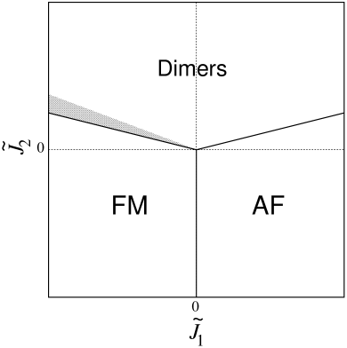
Figure 2: The phase diagram including nearest neighbor, next-nearest neighbor, and 3-particle ring exchanges. The effective couplings $\widetilde{J}_{1}$ and $\widetilde{J}_{2}$ are defined in the text. The shaded region between the dimer and ferromagnetic phases corresponds to the exotic phase predicted in Ref. Chubukov, .

Thus, depending on the relative magnitudes of the various exchange constants, different phases are realized. Extensive studies of the two-dimensional Wigner crystal have shown that, at low densities (or strong interactions), the 3-particle ring exchange dominates over the 2-particle exchanges. As a result, the two-dimensional Wigner crystal becomes ferromagnetic at sufficiently strong interactions.Roger ; Bernu Given that the electrons in a two-dimensional Wigner crystal form a triangular lattice, by analogy, one should expect a similar effect in the zigzag chain at densities where the electrons form approximately equilateral triangles. More specifically, upon increasing the density and consequently the distance between rows, one would expect the system to undergo a phase transition from an antiferromagnetic to a ferromagnetic phase. To establish this scenario conclusively, the various exchange energies in the zigzag crystal have to be determined. The system differs from the two-dimensional crystal in two important aspects. (i) The electrons are subject to a confining potential as opposed to the flat background in the two-dimensional case. Even more importantly, (ii) the electron configuration depends on density, cf. Fig. 1, as opposed to the ideal triangular lattice in two dimensions. In the following section, we proceed with a numerical study of the exchange energies for the specific configurations of the zigzag Wigner crystal in a parabolic confining potential.

IV Semiclassical evaluation of the exchange constants

The effective strength of interactions is usually described by the interaction parameter $r_{s}$ which measures the relative magnitude of the interaction energy and the kinetic energy and is of order the distance between electrons measured in units of the Bohr radius. For quantum wires, it is more appropriate to use the parameter $r_{\Omega}=r_{0}/a_{B}$, which takes into account the confining potential. Within our model, the interaction parameter $r_{\Omega}$ is

$$r_{\Omega}=2\left(\frac{me^{4}}{2\epsilon^{2}\hbar^{2}}\,\frac{1}{\hbar\Omega}\right)^{2/3}.$$ (8)

For $r_{\Omega}\gg 1$, strong interactions dominate the physics of the system, and a semiclassical description is applicable. In order to calculate the various exchange constants, we use the standard instanton method, successfully employed in the study of the two-dimensionalRoger ; Voelker ; Katano and one-dimensionalKRM ; Fogler Wigner crystal. Within this approach, the exchange constants are given by $J_{l}=J^{*}_{l}\exp{(-S_{l}/\hbar)}$. Here $S_{l}$ is the value of the Euclidean (imaginary time) action, evaluated along the classical exchange path. By measuring length and time in units of $r_{0}$ and $T=\sqrt{2}/\Omega$, respectively, the action $S[\{{\bf r}_{j}(\tau)\}]$ can be rewritten in the form $S=\hbar\eta\sqrt{r_{\Omega}}$, where the functional

$$\eta[\{{\bf r}_{j}(\tau)\}]=\!\int\limits_{-\infty}^{\infty}\!\!\mathrm{d}\tau\!\left[\sum_{j}\left(\frac{\dot{{\bf r}}_{j}^{2}}{2}+y_{j}^{2}\right)+\sum_{j<i}\frac{1}{|{\bf r}_{j}\!-\!{\bf r}_{i}|}\right]\!\!$$ (9)

is dimensionless.

Thus, we find the exchange constants in the form

$$J_{l}=J^{*}_{l}\exp{(-\eta_{l}\sqrt{r_{\Omega}})},$$ (10)

where the dimensionless coefficients $\eta_{l}$ depend only on the electron configuration (cf. Fig. 1) or, equivalently, on the density $\nu$. The exponents $\eta_{l}$ are calculated numerically for each type of exchange by minimizing the action (9) with respect to the instanton trajectories of the exchanging electrons. This procedure is mathematically equivalent to solving a set of coupled, second order in the imaginary time $\tau$, differential equations for the trajectories ${\bf r}_{j}(\tau)$. The boundary conditions at $\tau=\pm\infty$ are, respectively, the original equilibrium configuration and the configuration where the electrons have exchanged positions according to the exchange process considered.

Figure 3: The exponents $\eta_{1}$, $\eta_{2}$, $\eta_{3}$, and $\eta_{4}$ as functions of the dimensionless density $\nu$.

In the simplest approximation only the exchanging electrons are included in the calculation while all other electrons, being frozen in place, create the background potential. It turns out, however, that it is important to take into account the motion of “spectators”—the electrons in the crystal to the left and to the right of the exchanging particles—during the exchange process. The results presented here are obtained by successively adding more spectators on both sides until the values $\eta_{l}$ converge. We find that including 12 moving spectators on either side of the exchanging particles determines the exponents to an accuracy better than $0.1\%$.

$\nu$	$\eta_{1}$	$\eta_{2}$	$\eta_{3}$	$\eta_{4}$
1.0	1.050	2.427	1.254	1.712
1.1	1.161	2.169	1.261	1.605
1.2	1.255	1.952	1.275	1.532
1.3	1.337	1.754	1.287	1.469
1.4	1.406	1.566	1.293	1.398
1.5	1.456	1.376	1.278	1.299
1.6	1.471	1.169	1.215	1.135
1.7	1.391	0.901	1.022	0.784

Table 1: The numerically calculated values of the density dependent exponents $\eta_{l}$, see Eq. (10). The computation was carried out including 12 moving spectator particles on either side of the exchanging particles. Corrections to all $\eta_{l}$ from the remaining spectators do not exceed $0.1\%$.

Figure 3 shows the calculated exponents for various exchanges as a function of dimensionless density $\nu$ and the corresponding values are reported in Table 1. At strong interactions ($r_{\Omega}\gg 1$), the exchange with the smallest value of $\eta_{l}$ is clearly dominant, and the prefactor $J^{*}_{l}$ is of secondary importance to our argument. At low densities, when the zigzag chain is still close to one-dimensional, $J_{1}$ is the largest exchange constant, and the spin physics is controlled by the nearest-neighbor exchange. In an intermediate density regime, when the electron configuration is close to equilateral triangles, the 3-particle ring exchange dominates. Thus, the numerical calculation confirms our original expectation, and a transition from an antiferromagnetic to a ferromagnetic state takes place upon increasing the density. Surprisingly, however, at even higher densities the 4-particle ring exchange is the dominant process. The role of the 4-particle ring exchange and the phase diagram of the associated zigzag spin chain will be the subject of the following section. More complicated exchanges have also been computed, namely multi-particle ($l\geq 5$) ring exchanges as well as exchanges involving more distant neighbors. However, the exchanges displayed in Fig. 3 were found to be the dominant ones.us

It is important to note here that spectators contribute to our results in an essential way. Allowing spectators to move results not only in quantitative changes (namely a reduction of the initially overestimated values $\eta_{l}$) but in qualitative changes as well: at high densities, the dominance of the 4-particle ring exchange $J_{4}$ over the next-nearest neighbor exchange $J_{2}$ is obtained only if spectators are taken into account. In particular, it is necessary to include at least 6 moving spectators on each side of the exchanging particles for $J_{4}$ to take over at high densities.

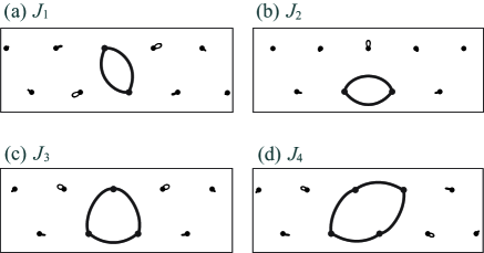
Figure 4: The calculated particle trajectories for various exchanges at a representative density $\nu=1.5$. It is evident that only a few near neighbors of the exchanging particles move appreciably.

The considerable effect that the spectators have on the values of the exponents raises the question whether a short-ranged interaction potential might cause further quantitative or qualitative changes to the physical picture. In order to investigate that possibility we have repeated the entire calculation for a modified Coulomb interaction of the form

$$V(x)=\frac{e^{2}}{\epsilon}\left(\frac{1}{|x|}-\frac{1}{\sqrt{x^{2}+(2d)^{2}}}\right).$$ (11)

This particular interaction accounts for the presence of a metal gate, modeled by a conducting plane at a distance $d$ from the crystal. The gate screens the bare Coulomb potential, modifying the electron-electron interaction at long distances. Our calculation shows that this modification affects the values of the exponents only weakly, even when the gate is placed at a distance from the crystal comparable to the inter-particle spacing. Qualitatively, the physical picture remains the same, with the order of dominance of the various exchanges unaffected throughout the range of densities.

At the same time, it is particularly noteworthy that (both for the screened and unscreened interaction) the contribution of the spectator electrons saturates rapidly as their number is increased. This is an indication that the destruction of long-range order in the quasi-one-dimensional Wigner crystal by quantum fluctuations will not affect our conclusions. Figure 4 shows the particle trajectories for the dominant exchanges at a representative density of $\nu=1.5$. The trajectories of both the exchanging particles and a subset of the spectators are shown, and their relative displacements can be readily compared.

V Four-particle ring exchange

We have shown in the preceding section that in a certain range of densities, the 4-particle ring exchange dominates. Unlike the 3-particle exchange, the 4-particle ring exchange not only modifies the nearest and next-nearest neighbor exchange constants, but, in addition, introduces more complicated spin interactions.Thouless For the zigzag chain, we find

$$\!\!H_{4} \!\!=\!\! J_{4}\sum_{j}\Big{(}\sum_{l=1}^{3}\frac{4-l}{2}{\bf S}_{j}{\bf S}_{j\!+\!l}+2\big{[}({\bf S}_{j}{\bf S}_{j\!+\!1})({\bf S}_{j\!+\!2}{\bf S}_{j\!+\!3})$$ (12)

$$+({\bf S}_{j}{\bf S}_{j\!+\!2})({\bf S}_{j\!+\!1}{\bf S}_{j\!+\!3})-({\bf S}_{j}{\bf S}_{j\!+\!3})({\bf S}_{j\!+\!1}{\bf S}_{j\!+\!2})\big{]}\Big{)}.$$

Not much is known about the physics of zigzag spin chains with interactions of this type. We have studied this particular system described by the Hamiltonian $H=H_{123}+H_{4}$ using exact diagonalization, considering systems of $N=12,16,20,24$ sites. Periodic boundary conditions have been imposed, and we have employed the well-known Lanczos algorithm to calculate a few low-energy eigenstates.

Figure 5: Total spin $S$ of the ground state for a chain of $N=24$ sites as a function of the effective couplings $\widetilde{J}_{1}/J_{4}$ and $\widetilde{J}_{2}/J_{4}$.

Figure 5 shows the total spin $S$ of the ground state as a function of the effective couplings $\widetilde{J}_{1}/J_{4}$ and $\widetilde{J}_{2}/J_{4}$ for the largest system considered, one with $N=24$ sites. The darkest region corresponding to maximal total spin is the ferromagnetic phase, which occurs for large negative couplings in direct analogy to the phase diagram for the system without four-spin interactions (see Fig. 2). For all system sizes that we have considered, the obtained phase boundary is almost independent of the system size and agrees very well with the conditions for ferromagnetism

$$\widetilde{J}_{1}+2J_{4} <0,$$ (13)

$$\widetilde{J}_{1}+4\widetilde{J}_{2}+10J_{4} <0,$$ (14)

derived by treating the four-spin terms in the Hamiltonian (12) on a mean field level near the ferromagnetic state.

A new phase of partial spin polarization appears adjacent to the ferromagnetic phase. The partially polarized phase possesses a ground state total spin of $S=2$ for $N=12$, $S=2$ or 4 for $N=16,20$, and $S=4$ for $N=24$; it appears that total spin of one third of the saturated magnetization $N/2$ prevails throughout most of that phase. The phase persists, to a significant extent, in range and form as $N$ increases. Therefore, we believe it is not a finite size effect. We note here that it has been shown rigorously that a model described by a Hamiltonian having a similar form to ours also exhibits a ground state with partial spin polarization.Muramoto On the other hand, the scattered points corresponding to non-zero total spin in the first quadrant ($\widetilde{J}_{1},\widetilde{J}_{2}>0$) appear to shift position as $N$ increases and the size of the total spin remains small, $S\leq 2$, for all system sizes considered. We cannot ascertain at this point whether they persist in a larger system.

Figure 6: Overlaps of the ground state wavefunctions in the presence of the 4-particle ring exchange with the wavefunctions representing (a) the dimer and (b) the antiferromagnetic phase for $J_{4}=0$. The representative ground states (a) and (b) are obtained for $(\widetilde{J}_{1},\widetilde{J}_{2},J_{4})=(1,10,0)$ and $(\widetilde{J}_{1},\widetilde{J}_{2},J_{4})=(1,-10,0)$, respectively.

At large values of $|\widetilde{J}_{1}|/J_{4}$ and $|\widetilde{J}_{2}|/J_{4}$, one would expect to recover the phases present in the absence of $J_{4}$. Thus, the large white area in Fig. 5 corresponding to total spin $S=0$ should contain the antiferromagnetic phase, analogues of the dimer phases observed in the system without four-spin interactions, and possibly entirely new phases as well. In order to distinguish between these phases, we first calculate the overlap between the ground state wavefunctions in our model and the ones representing the dimer and antiferromagnetic phases in the well-studied model with $J_{4}=0$. The representative ground state wavefunctions are obtained for the chain with $J_{4}=0$ and typical parameter sets of $(\widetilde{J}_{1},\widetilde{J}_{2})$ chosen deep in the dimer and antiferromagnetic phases of the phase diagram shown in Fig. 2. The results for the chain with $N=24$ sites are shown in Fig. 6. As can be seen from the figure, the ground states for a broad region of large positive $\widetilde{J}_{2}/J_{4}$ have a significant overlap with the representative ground state of the dimer phase while the ground states for large positive $\widetilde{J}_{1}/J_{4}$ and/or negative $\widetilde{J}_{2}/J_{4}$ resemble very much the one belonging to the antiferromagnetic phase. This behavior indicates the appearance of the expected dimer and antiferromagnetic phases for large effective couplings $|\widetilde{J}_{1}|/J_{4}$ and $|\widetilde{J}_{2}|/J_{4}$. We have confirmed the existence of these phases in the corresponding parameter regimes by studying the associated structure factors.

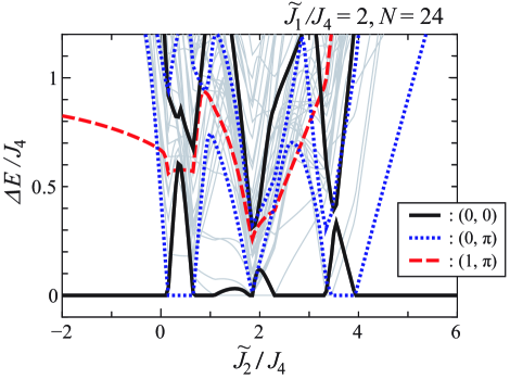
Figure 7: Excitation energies $\Delta E_{n}(S,Q)$ in the system of $N=24$ sites for $\widetilde{J}_{1}/J_{4}=2$ as functions of $\widetilde{J}_{2}/J_{4}$. The two-lowest levels are plotted for the subspaces of $(S,Q)=(0,0)$ and $(0,\pi)$ while only the lowest one is shown for all other subspaces. The energies for $(S,Q)=(0,0)$, $(0,\pi)$, and $(1,\pi)$ are plotted by thick solid, dotted, and dashed curves, respectively. The energies of the levels belonging to other subspaces are shown by thin gray curves.

In order to study and clarify the properties of the system in more detail, we have calculated the excitation energies

$$\Delta E_{n}(S,Q)=E_{n}(S,Q)-E_{\rm gs},$$ (15)

where $E_{n}(S,Q)$ is the energy of $n$-th lowest level in the subspace characterized by the total spin $S$ and the momentum $Q$, and $E_{\rm gs}$ is the ground state energy. Figure 7 shows the results for the system of size $N=24$, obtained along the vertical line in the phase diagram given by $\widetilde{J}_{1}/J_{4}=2$. At large positive $\widetilde{J}_{2}/J_{4}$, the ground and first-excited states belong to the subspace $(S,Q)=(0,0)$ and $(0,\pi)$, respectively.dimerdoublet-footnote These states are expected to form the ground state doublet of the dimer phase in the thermodynamic limit. For $\widetilde{J}_{2}/J_{4}>(\widetilde{J}_{2}/J_{4})_{c,{\rm dim}}\sim 3.5$, one of the dimer doublet states is the ground state and the system is in the dimer phase. At smaller $\widetilde{J}_{2}/J_{4}$, both states of the dimer doublet shift upward and move away from the low-energy regime, while other states decrease steeply in energy and eventually become the ground state. We therefore take the point $(\widetilde{J}_{2}/J_{4})_{c,{\rm dim}}$ as the boundary of the dimer phase. After the transition, the system enters a region with exotic ground states and a large number of low-lying excitations. We have numerically checked that these exotic ground states have no or, at most, negligibly small overlap with the ground state of either the dimer or antiferromagnetic phases. When $\widetilde{J}_{2}/J_{4}$ decreases further, the exotic states leave the low-energy regime and the system predictably enters the antiferromagnetic phase, which occurs for $\widetilde{J}_{2}/J_{4}<(\widetilde{J}_{2}/J_{4})_{c,{\rm AF}}\sim 0.1$.

Figure 8: The phase diagram of the Heisenberg chain including nearest neighbor, next-nearest neighbor, and 4-particle ring exchanges. The expected phases consist of a ferromagnetic and an antiferromagnetic phase as well as a dimer phase. In addition, a novel region ($4P$) dominated by the 4-particle ring exchange appears. The latter includes a phase of partial spin polarization ($M$). Triangles, squares and circles correspond to the boundaries obtained for $N=16$, 20, and 24 sites, respectively. We note that although the phase of partial spin polarization persists as the system size is increased, its boundary with the 4P phase has a rather irregular size dependence and is represented approximately in the figure.

Performing the same type of analysis for several parameter lines, we can estimate the phase boundaries $(\widetilde{J}_{2}/J_{4})_{c,{\rm dim}}$ and $(\widetilde{J}_{2}/J_{4})_{c,{\rm AF}}$ as functions of $\widetilde{J}_{1}/J_{4}$. In the limit of large negative coupling $\widetilde{J}_{1}/J_{4}\to-\infty$, the boundary of the dimer phase $(\widetilde{J}_{2}/J_{4})_{c,{\rm dim}}$ approaches the line $\widetilde{J}_{1}=-0.38\widetilde{J}_{2}$, suggesting a smooth connection to the behavior for $\widetilde{J}_{1}<0$ and $J_{4}=0$ (cf. Ref. Chubukov, ). In a similar fashion, at large positive coupling $\widetilde{J}_{1}/J_{4}$, we find no indication for the appearance of exotic phases after $\widetilde{J}_{1}/J_{4}\geq 6$; the data of the energy spectrum and the wavefunction overlaps show essentially the same behaviors as those at $\widetilde{J}_{1}/J_{4}\to\infty$. We therefore conclude that there occurs a direct transition between the dimer and antiferromagnetic phases and estimate the transition line using the method of level spectroscopy, according to which the transition point is determined by the level crossing between the first-excited states in the dimer and antiferromagnetic phases.Okamoto

Combining all these phase boundaries and including the boundaries of the ferromagnetic and partially spin polarized phases which were obtained using the total spin of the ground state as a criterion, we determine the phase diagram in the $\widetilde{J}_{1}/J_{4}$ versus $\widetilde{J}_{2}/J_{4}$ plane. The result is shown in Fig. 8. The phase diagram has similarities to the one obtained without the four-spin interaction term, see Fig. 2. In particular, the expected ferromagnetic, antiferromagnetic, and dimer phases appear for large values of the effective couplings, $|\widetilde{J}_{1}|/J_{4}$ and $|\widetilde{J}_{2}|/J_{4}$. But more importantly, at not too large values of the effective couplings, new phases appear as a direct result of the new interaction term. We can identify a phase with partial spin polarization and a region occupied by one or several novel phases with total spin $S=0$. In the region where $J_{4}$ dominates, the ground state has no similarity at the level of wavefunctions with that of the conventional phases. It is important to note that the region occupied by the new phases becomes broader as the system size $N$ grows, indicating that it survives even in the thermodynamic limit. From the analysis of the wavefunction overlaps between the ground states, there are strong indications that the novel unpolarized region might consist of several different phases. Unfortunately, it has proven difficult to clarify the nature of the new phases and, in particular, discover the order parameters that characterize them based solely on the analysis of small systems. Therefore, the issue is relegated to future studies. In the absence of detailed understanding of its properties, we collectively dub the region of the phase diagram the “4P” phase.

VI Phase diagram for realistic quantum wires

Having identified possible phases of the zigzag chain, the most interesting question is which of the various phases appearing in the phase diagram Fig. 8 are accessible in quantum wires. At finite $r_{\Omega}$, the calculations of the exchange constants discussed in Sec. IV have to be completed in an important way by computing the prefactors $J_{l}$ in Eq. (10). To that effect it is necessary to take into account Gaussian fluctuations around the classical exchange path. We employ the method introduced by Voelker and ChakravartyVoelker which, for the sake of completeness, is outlined in the Appendix A. The prefactors have the form

$$J^{*}_{l}=\frac{e^{2}}{\epsilon a_{B}}\,A_{l}F_{l}\,{r_{\Omega}}^{-\frac{5}{4}}\sqrt{\frac{\eta_{l}}{2\pi}},$$ (16)

where $F_{l}$ is density dependent. The factor $A_{l}$ is used to account for multiple classical trajectories corresponding to the same exchange process (see Appendix). Table 2 contains the values of $F_{l}$ we calculated for the various exchanges considered in this work. Note that, in order to achieve a comparable level of convergence, a more accurate determination of the instanton trajectories was required for the calculation of the prefactors $J^{*}_{l}$ than for the calculation of the exponents $\eta_{l}$. By including up to 28 moving spectators on either side of the exchanging particles, we have been able to achieve an accuracy better than 2%.

$\nu$	$F_{1}$	$F_{2}$	$F_{3}$	$F_{4}$
1.0	1.12	$\simeq 6$	1.22	2.44
1.1	1.04	$\simeq 4$	1.03	1.73
1.2	1.05	2.38	0.97	1.28
1.3	1.08	1.86	0.97	1.15
1.4	1.19	1.71	1.02	1.13
1.5	1.40	1.63	1.14	1.18
1.6	1.80	1.51	1.26	1.19
1.7	2.07	1.07	0.81	0.50

Table 2: The numerically calculated values of the density dependent part $F_{l}$ of the exchange energy prefactor $J^{*}_{l}$, see Eq. (16), calculated with mobile spectators. For all the numbers reported, the accuracy is better than 2%, except for $F_{2}$ at $\nu=1.0$, $1.1$, for which extrapolated values with an estimated error of $\sim 10\%$ are shown.

We are now in a position to map out the areas of the phase diagram of Fig. 8 that are encountered as one traverses the density region of interest for a given $r_{\Omega}$. The resulting phase diagram obtained with the calculated exchange energies is shown in Fig. 9. Since the semiclassical approximation is applicable only at $r_{\Omega}\gg 1$, we do not extend the phase diagram to values of $r_{\Omega}<10$. It turns out that the spin polarized phases are only realized at $r_{\Omega}\gtrsim 50$. On the other hand, the novel “4P” phase is expected to appear in a certain density range as long as $r_{\Omega}\gg 1$.

Figure 9: The phase diagram as a function of the dimensionless density $\nu$ and interaction strength $r_{\Omega}$. The various phases were obtained by first calculating the effective couplings $\widetilde{J}_{1}/J_{4}$ and $\widetilde{J}_{2}/J_{4}$ for a given point; subsequently, the corresponding phase was determined utilizing the calculated boundaries shown in Fig. 8 for a system of $N=24$ sites.

VII Discussion

In the preceding sections we have studied the coupling of spins of electrons forming a zigzag Wigner crystal in a parabolic confining potential. We have found that apart from the 2-particle exchange couplings between the nearest and next-nearest neighbor spins, the 3- and 4-particle ring exchange processes have to be taken into account. At relatively low electron densities, when the transverse displacement of electrons is small compared to the distance between particles, Fig. 1(b), the nearest-neighbor 2-particle exchange dominates. In this regime the spins form an antiferromagnetic ground state, with low-energy excitations described by the Tomonaga-Luttinger theory. At relatively high densities, when the transverse displacements are large, Fig. 1(c), the 4-particle ring exchange processes dominate. Since the ring exchange processes involving even numbers of particles favor spin-unpolarized states, the ground state of the system in this regime has zero total spin. Finally, if the confining potential is sufficiently shallow, so that the parameter $r_{\Omega}\gtrsim 50$, there is an intermediate density range in which the 3-particle exchange processes are important, and the ground state is spontaneously spin-polarized. These results are summarized in Fig. 9.

We expect that the zigzag Wigner crystal state can be realized in quantum wires. In order for the zigzag crystal to form the confining potential of the wire should be rather shallow, so that large values $r_{\Omega}\gg 1$ of the parameter (8) could be achieved. The exact shape of the confining potential in existing wires is not well known. Using the quoted value of subband spacing $\sim 20$ meV we estimate that the parameter $r_{\Omega}$ is of order unity in cleaved-edge-overgrowth wires.yacoby The confining potential in split-gate quantum wires tends to be more shallow. For a typical value 1 meV of subband spacing we estimate $r_{\Omega}\approx 6$. Finally, for p-type quantum wiresklochan ; daneshvar with subband spacing $\sim 300~{}\mu$eV we estimate $r_{\Omega}\approx 20$. These hole systems are the most promising devices for observation of the zigzag Wigner crystal.

Given the relatively modest values of $r_{\Omega}\lesssim 20$ in the existing quantum wire structures, we do not expect that the spontaneously spin-polarized ground state will be easily observed in experiments. Instead, we expect that as the density of charge carriers is increased, a transition from antiferromagnetism to a state dominated by 4-particle ring exchanges will occur. We have found that the ground state in this phase has a complicated size dependence, which makes it very difficult to identify its nature by exact diagonalization of finite-size chains. To fully understand the spin properties in the high density regime, further studies of zigzag ladders with ring exchange coupling are needed.

Appendix A Calculation of the prefactors

In order to find the prefactors $J_{l}^{*}$ in the expressions for the exchange constants, fluctuations around the instanton trajectory have to be taken into account. The Euclidean (imaginary time) path integral for the propagator $G({\bf R}_{1},{\bf R}_{2};T)=\langle{\bf R}_{1}|e^{-TH}|{\bf R}_{2}\rangle$ can be written as

$$G({\bf R}_{1},{\bf R}_{2};T)=\int_{{\bf R}(0)={\bf R}_{1}}^{{\bf R}(T)={\bf R}_{2}}\!\!\!\mathcal{D}{\bf R}\,e^{-\frac{1}{\hbar}S[{\bf R}]},$$ (17)

where the Euclidean action is given by

$$S[{\bf R}]=\int_{0}^{T}\!\!\!\mathrm{d}\tau\left\{\frac{m}{2}\left(\frac{\mathrm{d}{\bf R}}{\mathrm{d}\tau}\right)^{2}+V({\bf R})\right\}.$$ (18)

Here ${\bf R}$ is a $M$-dimensional position vector, where $M/2$ is the total number of moving particles, including the exchanging particles as well as the spectators. In the semiclassical limit, the integral is dominated by the classical path ${\bf R}_{cl}(\tau)$ that extremizes the action $S$ for a given exchange process. (The exponents $\eta$ are given as $\eta=S[{\bf R}_{cl}]/(\hbar\sqrt{r_{\Omega}})$.) The Gaussian quantum fluctuations about the classical path can be taken into account by defining fluctuation coordinates ${\bf u}(\tau)\equiv{\bf R}(\tau)-{\bf R}_{cl}(\tau)$ and subsequently expanding the action to second order. We obtain for the propagator

$$G({\bf R}_{1},{\bf R}_{2};T)=F[{\bf R}_{cl}]e^{-\frac{1}{\hbar}S[{\bf R}_{cl}]},$$ (19)

$$F[{\bf R}_{cl}]=\int_{{\bf u}(0)=0}^{{\bf u}(T)=0}\!\!\!\mathcal{D}{\bf u}(\tau)\,e^{-\frac{1}{\hbar}\delta S[{\bf u}(\tau)]},$$ (20)

$$\delta S[{\bf u}(\tau)]=\frac{m}{2}\int_{0}^{T}\!\!\mathrm{d}\tau\left\{\dot{{\bf u}}^{2}(\tau)+{\bf u}^{T}(\tau)\mathcal{H}(\tau){\bf u}(\tau)\right\},$$ (21)

$$\mathcal{H}_{kp}(\tau)=\frac{1}{m}\left.\frac{\partial^{2}V({\bf R})}{\partial R_{k}\partial R_{p}}\right|_{{\bf R}={\bf R}_{cl}(\tau)}.$$ (22)

In the preceding formulas, ${\bf R}_{1}$ and ${\bf R}_{2}$ correspond to two configurations of electrons that minimize the electrostatic potential $V({\bf R})$ describing electron-electron interactions as well as the confining potential. The exchange constant is related to the ratio of the propagator for a particular exchange process ${\bf R}_{1}\rightarrow{\bf R}_{2}$, divided by the propagator for the trivial path ${\bf R}_{cl}(\tau)={\bf R}_{1}$:

$$G=\frac{F[{\bf R}_{cl}]}{F[{\bf R}_{1}]}\,e^{-\frac{1}{\hbar}S[{\bf R}_{cl}]}.$$ (23)

We start from the expression for the propagator in the semiclassical limit and proceed by partitioning the time interval $[0,T]$ into $N$ subintervals $(\tau_{0},\tau_{1})$, $(\tau_{1},\tau_{2})$, $\dots$, $(\tau_{N-1},\tau_{N})$, with $\tau_{0}=0$, $\tau_{N}=T$. The partition is chosen sufficiently fine as to enable the approximation that in each subinterval, the Hessian matrix $\mathcal{H}(\tau)$ of the second derivative of the potential can be considered time independent, $\mathcal{H}(\tau)\simeq\mathcal{H}(\tau_{\nu})\equiv\mathcal{H}^{\nu}$. (In what follows, we use the convention that for the fluctuation coordinates, superscripts denote time subinterval, while subscripts denote spatial coordinate.) Subsequently the path integral is calculated as a product of path integrals over the partitioned interval. Moreover, each individual path integral is that of a multidimensional harmonic oscillator, for which analytic results exist. We then have

$$F[{\bf R}_{cl}]=\int\!\!\mathrm{d}{\bf u}^{1}\,G_{1}({\bf u}^{1},{\bf u}^{0};\tau_{1}-\tau_{0})\dots\int\!\!\mathrm{d}{\bf u}^{N-1}\,G_{N-1}({\bf u}^{N-1},{\bf u}^{N-2};\tau_{N-1}-\tau_{N-2})\,G_{N}({\bf u}^{N},{\bf u}^{N-1};\tau_{N}-\tau_{N-1}),$$ (24)

and the propagator for each subinterval is

$$G_{\nu}({\bf u}^{\nu},{\bf u}^{\nu-1};\tau_{\nu}-\tau_{\nu-1})=\int_{{\bf u}(\tau_{\nu-1})={\bf u}^{\nu-1}}^{{\bf u}(\tau_{\nu})={\bf u}^{\nu}}\!\!\!\mathcal{D}{\bf u}(\tau)\,\exp\left\{-\frac{m}{2\hbar}\int_{\tau_{\nu-1}}^{\tau_{\nu}}\!\!\mathrm{d}\tau\left[\dot{{\bf u}}^{2}(\tau)+{\bf u}^{T}(\tau)\mathcal{H}^{\nu}{\bf u}(\tau)\right]\right\}.$$ (25)

Within each imaginary time subinterval, we define orthonormal eigenvectors $q_{\mu}^{\nu}=\sum_{k=1}^{M}U^{\nu}_{k\mu}u_{k}^{\nu}$. The unitary matrix $U^{\nu}$ is such that $\mathcal{H}^{\nu}=U^{\nu}\Lambda^{\nu}(U^{\nu})^{T}$, with $\Lambda$ a diagonal matrix of eigenvalues $(\lambda^{\nu}_{\mu})^{2}$, $\mu=1\dots M$, where $M$ is the number of spatial coordinates. Then one immediately obtains

$$G_{\nu}({\bf q}^{\nu},{\bf q}^{\nu-1};\tau_{\nu}-\tau_{\nu-1})=\int_{{\bf q}(\tau_{\nu-1})={\bf q}^{\nu-1}}^{{\bf q}(\tau_{\nu})={\bf q}^{\nu}}\!\!\!\mathcal{D}{\bf q}(\tau)\,\exp\left\{-\frac{m}{2\hbar}\int_{\tau_{\nu-1}}^{\tau_{\nu}}\!\!\mathrm{d}\tau\left[\dot{{\bf q}}^{2}(\tau)+{\bf q}^{T}(\tau)\Lambda^{\nu}{\bf q}(\tau)\right]\right\}=\bar{F}[{\bf q}_{cl}]e^{-\frac{1}{\hbar}\delta S[{\bf q}_{cl}]},$$ (26)

where ${\bf q}_{cl}$ is the classical trajectory connecting ${\bf q}^{\nu-1}$ and ${\bf q}^{\nu}$. Considering the fluctuation part first, we obtain an elementary path integral

$$\bar{F}[{\bf q}_{cl}]=\int_{{\bf q}(\tau_{\nu-1})=0}^{{\bf q}(\tau_{\nu})=0}\!\!\!\mathcal{D}{\bf q}(\tau)\,\exp\left\{-\frac{m}{2\hbar}\int_{\tau_{\nu-1}}^{\tau_{\nu}}\!\!\mathrm{d}\tau\,{\bf q}^{T}(\tau)\left[-\frac{\mathrm{d}^{2}}{\mathrm{d}\tau^{2}}+\Lambda^{\nu}\right]{\bf q}(\tau)\right\}=\prod_{\mu=1}^{M}\sqrt{\frac{B_{\mu}^{\nu}}{2\pi}},$$ (27)

where

$$B_{\mu}^{\nu}=\frac{m\lambda_{\mu}^{\nu}}{\hbar\sinh(\lambda^{\nu}_{\mu}\Delta\tau_{\nu})},$$ (28)

and $\Delta\tau_{\nu}=\tau_{n}-\tau_{n-1}$. The exponent $\delta S[{\bf q}_{cl}]$ can now be calculated explicitly

$$\frac{\delta S[{\bf q}_{cl}]}{\hbar} =\frac{1}{2}\sum_{\mu=1}^{M}B_{\mu}^{\nu}\left\{[(q_{\mu}^{\nu})^{2}_{cl}+(q_{\mu}^{\nu-1})^{2}_{cl}]\cosh(\lambda^{\nu}_{\mu}\Delta\tau_{\nu})\right.$$

$$\phantom{\frac{1}{2}\sum_{\mu=1}^{M}B_{\mu}^{\nu}\left\{\right\}}\left.-2(q_{\mu}^{\nu})_{cl}(q_{\mu}^{\nu-1})_{cl}\right\}.$$ (29)

The subscript “$cl$” used for notational clarity will be subsequently dropped from all expressions. With some additional algebra, the remaining integral is easily evaluated. With the following definitions

$$\Gamma_{kp}^{\nu} =\sum_{\mu=1}^{M}U^{\nu}_{k\mu}\frac{m\lambda^{\nu}_{\mu}}{\hbar\tanh(\lambda^{\nu}_{\mu}\Delta\tau_{\nu})}U^{\nu}_{p\mu}$$ (30)

$$\Delta_{kp}^{\nu} =\sum_{\mu=1}^{M}U^{\nu}_{k\mu}\frac{m\lambda^{\nu}_{\mu}}{\hbar\sinh(\lambda^{\nu}_{\mu}\Delta\tau_{\nu})}U^{\nu}_{p\mu},$$ (31)

we find

$$F[{\bf R}_{cl}]=(2\pi)^{-\frac{M}{2}}\prod_{\nu=1}^{N}\prod_{\mu=1}^{M}\sqrt{B_{\mu}^{\nu}}\frac{1}{\sqrt{\det\Omega}},$$ (32)

where the $M(N-1)\times M(N-1)$ matrix $\Omega_{kp}^{\nu\lambda}$ has components

$$\Omega_{kp}^{\nu\lambda}=(\Gamma_{kp}^{\nu}+\Gamma_{kp}^{\nu+1})\delta^{\nu,\lambda}-\Delta_{kp}^{\nu}\delta^{\nu,(\lambda+1)}-\Delta_{kp}^{\lambda}\delta^{\nu,(\lambda-1)}.$$ (33)

The calculation of $F[{\bf R}_{1}]$ is carried out in an identical manner and the subscript “0” will be used to distinguish the results pertaining to that calculation.

Finally, one has to account for the existence of an eigenvalue of the matrix $\Omega$ which is identically zero in the continuum limit and corresponds to the zero mode associated with uniform translation of the instanton in imaginary time. The procedure is standardColeman and we simply report the result for the prefactor here. One obtains

$$G=T\left(\frac{S}{2\pi\hbar m}\right)^{\frac{1}{2}}\displaystyle\prod_{\nu=1}^{N}\prod_{\mu=1}^{M}\sqrt{\frac{B_{\mu}^{\nu}}{B_{\mu,0}^{\nu}}}\sqrt{\frac{\det\Omega_{0}}{\det^{\prime}\Omega}},$$ (34)

where the primed determinant implies the exclusion of the eigenvalue corresponding to the zero mode. Reverting to the system of units used in this work, the prefactor of the exchange energy is given by

$$J^{*}_{l}=\frac{e^{2}}{\epsilon a_{B}}\,A_{l}\,{r_{\Omega}}^{-\frac{5}{4}}\sqrt{\frac{\eta_{l}}{2\pi}}\displaystyle\prod_{\nu=1}^{N}\prod_{\mu=1}^{M}\sqrt{\frac{B_{\mu}^{\nu}}{B_{\mu,0}^{\nu}}}\sqrt{\frac{\det\Omega_{0}}{\det^{\prime}\Omega}}.$$ (35)

The additional factor $A_{l}$ is used to account for multiple classical trajectories corresponding to the same exchange process, as happens for the case of nearest and next-nearest neighbor exchanges (i.e., $A_{1}=A_{2}=2$, whereas $A_{l}=1$ for $l\geq 3$).

The numerical implementation of the method outlined above is straightforward. In particular, the quantity that needs to be numerically calculated, once for each type of exchange at all densities of interest, is

$$F_{l}=\displaystyle\prod_{\nu=1}^{N}\prod_{\mu=1}^{M}\sqrt{\frac{B_{\mu}^{\nu}}{B_{\mu,0}^{\nu}}}\sqrt{\frac{\det\Omega_{0}}{\det^{\prime}\Omega}}.$$ (36)

We note here that the eigenvalue corresponding to the zero mode is easily calculated with the same procedure used by Voelker and ChakravartyVoelker . In the definition of the prefactor, see Eqs. (20) and (21), one replaces $\mathcal{H}(\tau)$ with $\mathcal{H}(\tau)-\lambda$, with $\lambda$ a free parameter. Subsequently, a numerical search for the smallest eigenvalue that results in $1/F(\lambda)=0$ is carried out. The smallest eigenvalue corresponds to the zero mode, and for a finite partition of the imaginary time interval it is a small but finite number.

References

- (1) K. J. Thomas, J. T. Nicholls, M. Y. Simmons, M. Pepper, D. R. Mace, and D. A. Ritchie, Phys. Rev. Lett. 77, 135 (1996).
- (2) A. Kristensen, J. B. Jensen, M. Zaffalon, C. B. Sørensen, S. M. Reimann, P. E. Lindelof, M. Michel, and A. Forchel, J. Appl. Phys. 83, 607 (1998).
- (3) A. Kristensen, H. Bruus, A. E. Hansen, J. B. Jensen, P. E. Lindelof, C. J. Marckmann, J. Nygård, C. B. Sørensen, F. Beuscher, A. Forchel, and M. Michel, Phys. Rev. B 62, 10950 (2000).
- (4) K. J. Thomas, J. T. Nicholls, N. J. Appleyard, M. Y. Simmons, M. Pepper, D. R. Mace, W. R. Tribe, and D. A. Ritchie, Phys. Rev. B 58, 4846 (1998).
- (5) B. E. Kane, G. R. Facer, A. S. Dzurak, N. E. Lumpkin, R. G. Clark, L. N. Pfeiffer, and K. W. West, Appl. Phys. Lett. 72, 3506 (1998).
- (6) K. J. Thomas, J. T. Nicholls, M. Pepper, W. R. Tribe, M. Y. Simmons, and D. A. Ritchie, Phys. Rev. B 61, R13365 (2000).
- (7) D. J. Reilly, G. R. Facer, A. S. Dzurak, B. E. Kane, R. G. Clark, P. J. Stiles, R. G. Clark, A. R. Hamilton, J. L. O’Brien, N. E. Lumpkin, L. N. Pfeiffer, and K. W. West, Phys. Rev. B 63, 121311(R) (2001).
- (8) S. M. Cronenwett, H. J. Lynch, D. Goldhaber-Gordon, L. P. Kouwenhoven, C. M. Marcus, K. Hirose, N. S. Wingreen, and V. Umansky, Phys. Rev. Lett. 88, 226805 (2002).
- (9) D. J. Reilly, T. M. Buehler, J. L. O’Brien, A. R. Hamilton, A. S. Dzurak, R. G. Clark, B. E. Kane, L. N. Pfeiffer, and K. W. West, Phys. Rev. Lett. 89, 246801 (2002).
- (10) R. Crook, J. Prance, K. J. Thomas, S. J. Chorley, I. Farrer, D. A. Ritchie, M. Pepper, and C. G. Smith, Science 312, 1359 (2006).
- (11) R. de Picciotto, L. N. Pfeiffer, K. W. Baldwin, and K. W. West, Phys. Rev. B 72, 033319 (2005).
- (12) R. Danneau, W. R. Clarke, O. Klochan, A. P. Micolich, A. R. Hamilton, M. Y. Simmons, M. Pepper, and D. A. Ritchie, Appl. Phys. Lett. 88, 012107 (2006).
- (13) O. Klochan, W. R. Clarke, R. Danneau, A. P. Micolich, L. H. Ho, A. R. Hamilton, K. Muraki, and Y. Hirayama, Appl. Phys. Lett. 89, 092105 (2006).
- (14) L. P. Rokhinson, L. N. Pfeiffer, and K. W. West, Phys. Rev. Lett. 96, 156602 (2006).
- (15) C.-K. Wang and K.-F. Berggren, Phys. Rev. B 54, R14257 (1996); 57, 4552 (1998); A. A. Starikov, I. I. Yakimenko, and K.-F. Berggren, Phys. Rev. B 67, 235319 (2003).
- (16) B. Spivak and F. Zhou, Phys. Rev. B 61, 16730 (2000).
- (17) V. V. Flambaum and M. Yu. Kuchiev, Phys. Rev. B 61, R7869 (2000).
- (18) T. Rejec, A. Rams̆ak, and J. H. Jefferson, Phys. Rev. B 62, 12985 (2000).
- (19) H. Bruus, V. V. Cheianov, and K. Flensberg, Physica E 10, 97 (2001).
- (20) K. Hirose, S. S. Li, and N. S. Wingreen, Phys. Rev. B 63, 033315 (2001).
- (21) O. P. Sushkov, Phys. Rev. B 64, 155319 (2001); Phys. Rev. B 67, 195318 (2003).
- (22) Y. Meir, K. Hirose, and N. S. Wingreen, Phys. Rev. Lett. 89, 196802 (2002).
- (23) Y. Tokura and A. Khaetskii, Physica E 12, 711 (2002).
- (24) K. A. Matveev, Phys. Rev. Lett. 92, 106801 (2004); Phys. Rev. B 70, 245319 (2004).
- (25) T. Rejec and Y. Meir, Nature 442, 900 (2006).
- (26) H. Bruus and K. Flensberg, Semicond. Sci. Technol. 13, A30 (1998).
- (27) G. Seelig and K. A. Matveev, Phys. Rev. Lett. 90, 176804 (2003).
- (28) E. Lieb and D. Mattis, Phys. Rev. 125, 164 (1962).
- (29) A. D. Klironomos, J. S. Meyer and K. A. Matveev, Europhys. Lett. 74, 679 (2006).
- (30) H. J. Schulz, Phys. Rev. Lett. 71, 1864 (1993).
- (31) R. W. Hasse and J. P. Schiffer, Ann. Phys. 203, 419 (1990).
- (32) G. Piacente, I. V. Schweigert, J. J. Betouras, and F. M. Peeters, Phys. Rev. B 69, 045324 (2004).
- (33) W. Häusler, Z. Phys. B 99, 551 (1996).
- (34) A. D. Klironomos, R. R. Ramazashvili, and K. A. Matveev, Phys. Rev. B 72, 195343 (2005).
- (35) M. M. Fogler and E. Pivovarov, Phys. Rev. B 72, 195344 (2005); J. Phys.: Condens. Matter 18, L7 (2006).
- (36) M. Roger, Phys. Rev. B 30, 6432 (1984).
- (37) M. Katano and D. S. Hirashima, Phys. Rev. B 62, 2573 (2000).
- (38) K. Voelker and S. Chakravarty, Phys. Rev. B 64, 235125 (2001).
- (39) B. Bernu, L. Candido, and D. M. Ceperley, Phys. Rev. Lett. 86, 870 (2001).
- (40) D. J. Thouless, Proc. Phys. Soc. London 86, 893 (1965).
- (41) C. K. Majumdar and D. K. Ghosh, J. Math. Phys. 10, 1388 (1969); 10, 1399 (1969).
- (42) F. D. M. Haldane, Phys. Rev. B 25, R4925 (1982).
- (43) K. Okamoto and K. Nomura, Phys. Lett. A 169, 433 (1992).
- (44) S. Eggert, Phys. Rev. B 54, R9612 (1996).
- (45) S. R. White and I. Affleck, Phys. Rev. B 54, 9862 (1996).
- (46) T. Hamada, J. Kane, S. Nakagawa, and Y. Natsume, J. Phys. Soc. Jpn. 57, 1891 (1988).
- (47) T. Tonegawa and I. Harada, J. Phys. Soc. Jpn. 58, 2902 (1989).
- (48) A. V. Chubukov, Phys. Rev. B 44, 4693 (1991).
- (49) D. Allen, F. H. L. Essler, and A. A. Nersesyan, Phys. Rev. B 61, 8871 (2000).
- (50) C. Itoi and S. Qin, Phys. Rev. B 63, 224423 (2001).
- (51) N. Muramoto and M. Takahashi, J. Phys. Soc. Jpn. 68, 2098 (1999).
- (52) To be precise, we have found that the ground state at large belongs to the subspace [] for [], where is an integer, while the first-excited state belongs to the subspace [].
- (53) A. Yacoby, H. L. Stormer, N. S. Wingreen, L. N. Pfeiffer, K. W. Baldwin, and K. W. West, Phys. Rev. Lett. 77, 4612 (1996).
- (54) A. J. Daneshvar, C. J. B. Ford, A. R. Hamilton, M. Y. Simmons, M. Pepper, and D. A. Ritchie, Phys. Rev. B 55, R13409 (1997).
- (55) S. Coleman, Aspects of Symmetry (Cambridge University Press, New York, 1988).