Correlation functions and excitation spectrum of the frustrated ferromagnetic spin-$\frac{1}{2}$ chain in an external magnetic field

Abstract

Magnetic field effects on the one-dimensional frustrated ferromagnetic chain are studied by means of effective field theory approaches in combination with numerical calculations utilizing Lanczos diagonalization and the density matrix renormalization group method. The nature of the ground state is shown to change from a spin-density-wave region to a nematic-like one upon approaching the saturation magnetization. The excitation spectrum is analyzed and the behavior of the single spin-flip excitation gap is studied in detail, including the emergent finite-size corrections.

I Introduction

The interest in helical and chiral phases of frustrated low-dimensional quantum magnets has been triggered by recent experimental results. While many copper-oxide based materials predominantly realize antiferromagnetic exchange interactions, several candidate materials with magnetic properties believed to be described by frustrated ferromagnetic chains have been identified,Hase04 ; Gibson04 ; Enderle05 ; Banks06 ; buettgen07 ; Drechsler07 including Rb₂Cu₂Mo₃O₁₂ (Ref. Hase04, ), LiCuVO₄ (Refs. Gibson04, ; Enderle05, ; Banks06, ; buettgen07, ), and Li₂ZrCuO₄ (Ref. Drechsler07, ). The frustrated antiferromagnetic chain is well-studied,review-frust-1D but the magnetic phase diagram of the model with ferromagnetic nearest-neighbor interactions remains a subject of active theoretical investigations.Chubukov91 ; Heidrich-Meisner06 ; Kuzian ; Dmitriev

In this work we consider a parameter regime that is in particular relevant for the low-energy properties of LiCuVO₄, corresponding to a ratio of $J_{1}\approx-0.3\,J_{2}$ between the nearest neighbor interaction $J_{1}$ and the frustrating next-nearest neighbor interaction $J_{2}>0$. As the interchain couplings for this material are an order of magnitude smaller than the intrachain ones,Enderle05 we analyze a purely one-dimensional (1D) model. Apart from mean-field based predictions, Chubukov91 the nature of the ground state in a magnetic field $h$ is not yet completely known. Therefore, combining the bosonization technique with a numerical analysis we determine ground-state properties and discuss the model’s elementary excitations.

The Hamiltonian for our 1D model reads:

$$H=\sum_{x=1}^{L}\left(J_{1}\vec{S}_{x}\cdot\vec{S}_{x+1}+J_{2}\vec{S}_{x}\cdot\vec{S}_{x+2}\right)-h\sum_{x}S_{x}^{z}\,,$$ (1)

where $\vec{S}_{x}$ represents a spin one-half operator at site $x$.

Bosonization has turned out to be the appropriate language for describing the regime $|J_{1}|\ll J_{2}$ of Eq. (1). This result has been established by studying the magnetization process yielding a good agreement between field theory and numerical data.Heidrich-Meisner06 The derivation of the effective field theory is summarized in Sec. II. Here, we extend on such comparison of analytical and numerical results and further confirm the predictions of field theory by analyzing several correlation functions in Sec. III. Then, in Sec. IV, we numerically compute the one- and two-spin flip excitation gaps and compare them to field-theory predictions. Finally, Sec. V contains a summary and a discussion of our results.

II Effective field theory

We start from an effective field theory describing the long-wavelength fluctuations of Eq. (1). In the limit of strong next-nearest neighbor interactions $J_{2}\gg|J_{1}|$, the spin operators can be expressed as:

$$S^{z}_{\alpha}(r) \sim m+c(m)\sin\big{\{}2k_{F}r+\sqrt{4\pi}\phi_{\alpha}\big{\}}+\cdots$$

$$S_{\alpha}^{-}(r) \sim (-1)^{r}{\rm e}^{-i\theta_{\alpha}\sqrt{\pi}}+\cdots\,.$$ (2)

$k_{F}=(\frac{1}{2}-m)\pi$ is the Fermi-wave vector and $\alpha=1,2$ enumerates the two chains of the zig-zag ladder. In relation with Eq. (1), note that $\vec{S}_{1}(r)=\vec{S}_{(x+1)/2}$ ($\vec{S}_{2}(r)=\vec{S}_{x/2}$) for $x$ odd (even). $\phi_{\alpha}$ and $\theta_{\alpha}$ are compactified quantum fields describing the out-of-plane and in-plane angles of fluctuating spins obeying Gaussian Hamiltonians:

$${\cal H}=\frac{v}{2}\int dx\,\Big{\{}\frac{1}{K}(\partial_{x}\phi_{\alpha})^{2}+K(\partial_{x}\theta_{\alpha})^{2}\Big{\}}\,,$$ (3)

with $[\phi_{\alpha}(x),\theta_{\alpha}(y)]=i\Theta(y-x)$, where $\Theta(x)$ is the Heaviside function. Sub-leading terms are suppressed in Eq. (II). $m$ is the magnetization of decoupled chains, related to the real magnetization $M$ of the zig-zag system by:

$$M\simeq m\left(1-\frac{2K(m)J_{1}}{\pi v(m)}\right)\,.$$ (4)

$K(m)$ and $v(m)$ are the Luttinger liquid (LL) parameter and the spin-wave velocity of the decoupled chains, respectively. The nonuniversal amplitude $c(m)$ appearing in the bosonization formulas (II) has been determined from density matrix renormalization group (DMRG) calculations.Hikihara04 Note that in our notation $M=1/2$ at saturation.

Now we perturbatively add the interchain coupling term to two decoupled chains, each of which is described by an effective Hamiltonian of the form Eq. (3) and fields $\phi_{i}$ and $\theta_{i}$, $i=1,2$. For convenience, we transform to the symmetric and antisymmetric combinations of the bosonic fields $\phi_{\pm}=(\phi_{1}\pm\phi_{2})/\sqrt{2}$ and $\theta_{\pm}=(\theta_{1}\pm\theta_{2})/\sqrt{2}$. In this basis and apart from terms ${\mathcal{H}}_{0}^{\pm}$ of the form (3), the effective Hamiltonian describing low-energy properties of Eq. (1) contains a single relevant interaction term with the bare coupling $g_{1}\propto J_{1}\ll v$:

$${\mathcal{H}}_{\rm eff}={\mathcal{H}}_{0}^{+}+{\mathcal{H}}_{0}^{-}+g_{1}\int dx\,\cos\big{(}k_{F}+\sqrt{8\pi}\phi_{-}\big{)}\,,$$ (5)

and the renormalized LL parameters $K_{\pm}$ are, in the weak coupling limit:

$$K_{\pm}=K\,\left(1\mp J_{1}\,\frac{K}{\pi\,v}\right)\,.$$ (6)

$K_{+}$ is the Luttinger-liquid parameter of the soft mode of the zig-zag ladder. The Hamiltonian (5) represents the minimal effective low-energy field theory describing the region $J_{2}\gg|J_{1}|$ of the frustrated FM spin-${1}/{2}$ chain for $M\neq 0$.Heidrich-Meisner06 ; Cabra98 The relevant interaction term $\cos\sqrt{8\pi}\phi_{-}$ opens a gap in the $\phi_{-}$ sector. Since $S_{x+1}^{z}-S_{x}^{z}\sim\partial_{x}\phi_{-}$, relative fluctuations of the two chains are locked. This implies that single-spin flips are gapped with a sine-Gordon gap in the sector describing relative spin fluctuations of the two-chain system.Heidrich-Meisner06 Gapless excitations come from the $\Delta S^{z}=2$ channel, i.e. only those excitations are soft where spins simultaneously flip on both chains. DMRG results show that this picture applies to a large part of the magnetic phase diagram.Heidrich-Meisner06

III Correlation functions

We now turn to the ground state properties of Eq. (1) as a function of magnetization, concentrating on several correlation functions in order to identify the leading instabilities. Note that our analysis is only valid if $M\neq 0$. Apart from a term representing the magnetization $M$ induced by the external field, the longitudinal correlation function shows an algebraic decay with distance $r$:

$$\langle S_{\alpha}^{z}(0)S_{\beta}^{z}(r)\rangle\simeq M^{2}+\frac{C_{1}\cos({2k_{F}r+(\alpha-\beta)k_{F}})}{2\pi^{2}r^{K_{+}}}-\frac{K_{+}}{8\pi^{2}r^{2}}\,.$$ (7)

The constants $C_{i}$, $i=1,2,3$, appearing here and in Eq. (9) will be determined through a comparison with numerical results.

In contrast to Eq. (7), the transverse $xy$-correlation functions decay exponentially reflecting the gapped nature of the single spin-flip excitations. Here we do not restrict ourselves to the equal-time expression only, because we will need non-equal time correlation functions to extract the finite-size corrections to the gap later on. We obtain:

$$\langle S_{\alpha}^{+}(0,0)S_{\beta}^{-}(r,\tau)\rangle\simeq\frac{\delta_{\alpha,\beta}(-1)^{r}{\rm e}^{-\Delta_{1}(M)\sqrt{\tau^{2}+r^{2}/v_{-}^{2}}}}{(r^{2}+v_{+}^{2}\tau^{2})^{\frac{1}{8K_{+}}}(r^{2}+v_{-}^{2}\tau^{2})^{\frac{1}{8K_{-}}}}\,,$$ (8)

where $\tau$ stands for the Euclidean time, $\Delta_{1}(M)$ is the $\Delta S^{z}=1$ gap, and $v_{\pm}\sim v\pm J_{1}/\pi$ in the weak coupling limit. The Kronecker delta strictly applies to the thermodynamic limit, while on the lattice an additional contribution for $\alpha\neq\beta$ exists.

It is noteworthy that, different from Eq. (8), the in-plane correlation functions involving bilinear spin combinations decay algebraically. This stems from the gapless nature of $\Delta S^{z}=2$ excitations. In fact, these are the slowest decaying correlators close to the saturation magnetization:

$$\langle S_{1}^{+}(r)S_{2}^{+}(r)\,S_{1}^{-}(0)S_{2}^{-}(0)\rangle\simeq\frac{C_{2}}{r^{1/K_{+}}}+\frac{C_{3}\cos(2k_{F}r)}{r^{K_{+}+{1}/{K_{+}}}}\,.$$ (9)

This result is reminiscent of a partially ordered state because the ordering tendencies in this correlation function are more pronounced than those of the corresponding single-spin correlation function Eq. (8). Therefore, we call the correlator (9) ‘nematic’. Furthermore, we will refer to a situation where Eq. (9) is the slowest decaying one among all correlation functions as a ‘nematic-like phase’.

By virtue of the exponential decay in (8), the correlator (9) is proportional to:

$$\langle(S_{1}^{+}(r)+S_{2}^{+}(r))^{2}\,(S_{1}^{-}(0)+S_{2}^{-}(0))^{2}\rangle\,.$$ (10)

The term $(S_{1}^{\alpha}+S_{2}^{\alpha})^{2}$ appearing in the case of the $S=\frac{1}{2}$ zig-zag ladder corresponds to the operator $(S^{\alpha})^{2}$ in the case of a $S=1$ chain. One can think of an effective $S=1$ spin formed from two neighboring $S=\frac{1}{2}$ spins coupled by the ferromagnetic interaction. A similar behavior of correlation functions, namely the exponential decay of in-plane spin components and the algebraic decay of their bilinear combinations, is encountered also in the $XY2$ phase of the anisotropic $S=1$ chainSchulz1 and in the spin-1 chain with biquadratic interactions, see, e.g., Ref. LST06, .

The algebraic decay of the nematic correlator as opposed to the exponential decay of (8) suggests that there are tendencies towards nematic ordering in this phase. Depending on the value of $K_{+}$ the dominant instabilities are either spin-density-wave ones for $K_{+}<1$ or nematic ones for $K_{+}>1$. From the result for $K_{+}$ given in Eq. (6) one can perturbatively evaluate the crossover value of $J_{1}$:

$$|J_{1,cr}|=\frac{\pi v(m)}{K(m)}\left(\frac{1}{K(m)}-1\right)\,.$$ (11)

For $J_{1}<J_{1,cr}$ the nematic correlator (9) is the slowest decaying one, i.e. one is in the nematic-like phase. The behavior of the cross-over line can be read off from the behavior of $K(m)$: $K(m)$ increases monotonically with $m$, tends to $K=1$ for $m\to 1/2$, and satisfies $K<1$ for $m<1/2$ (see, e.g., Refs. Totsuka97, ; CHP98, ). Therefore, we have $J_{1,cr}=0$ for $M=1/2$ with increasing ferromagnetic $|J_{1,cr}|$ for decreasing $M$. This means that for $J_{1}<0$ a regime opens at high $M$ where nematic correlations given by Eq. (9) dominate over spin-density-wave correlations given by Eq. (7), in agreement with Chubukov’s prediction.Chubukov91

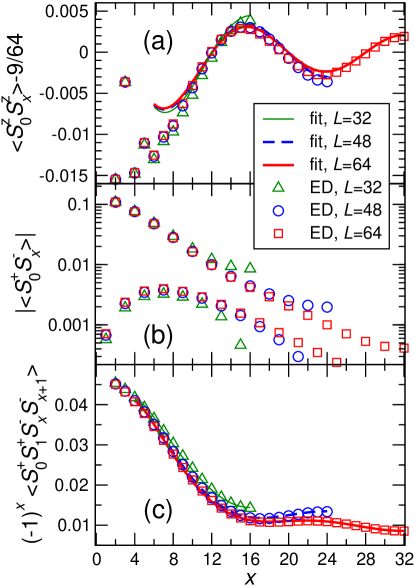
Figure 1: (Color online) Correlation functions at $J_{1}=-J_{2}<0$, and magnetization $M=3/8$: (a) longitudinal component $S^{z}_{x}$, (b) transverse component $S^{\pm}_{x}$, (c) spin nematic $S^{\pm}_{x}S^{\pm}_{x+1}$. $x$ is the distance in a single-chain notation. ED results for periodic boundary conditions are shown by symbols, fits by lines. Note the logarithmic scale of the vertical axis in panel (b).

Now we check the correlation functions obtained within bosonization against exact diagonalization (ED) results. Numerical data obtained for $J_{1}=-J_{2}<0$ and $M=3/8$ on finite systems with periodic boundary conditions are shown in Fig. 1. This parameter set allows for a clear test of the above predictions, but represents the generic behavior in the phase of two weakly coupled chains. To take into account finite-size effects we use the observation that for a conformally invariant theory, any power law on a plane becomes a power law in the following variable defined on a cylinder of circumference $L$:

$$x\to\frac{L}{\pi}\,\sin\left(\frac{x\,\pi}{L}\right)\,.$$ (12)

First we fit the nematic correlator given by Eq. (9), which from bosonization is expected to be the leading instability at high magnetizations. Using the part with $x\geq 5$ of the $L=64$ data shown in Fig. 1c, we find $1/K_{+}=0.904\pm 0.011$, $C_{2}=0.143\pm 0.004$, and $C_{3}=-0.326\pm 0.013$. Fig. 1c shows that all finite-size results for the nematic correlator are nicely described by this fit with the dependence on $L$ taken into account by substituting Eq. (12) for the power laws. Moreover, from $K_{+}>1$, we see that the system is indeed in the region dominated by nematic correlations for $M=3/8$ and $J_{1}=-J_{2}$.

Now we turn to the longitudinal correlation function which we fit to the bosonization result Eq. (7). Since most numerical parameters have been determined by the previous fit, only one free parameter is left which we determine from the numerical results of Fig. 1a for $L=64$ and $x\geq 14$ as $C_{1}=0.060\pm 0.004$. Predictions for other system sizes are again obtained by substituting Eq. (12) for the power laws. The agreement in Fig. 1a is not as good as in Fig. 1c. However, it improves at larger distances $x$ and system sizes $L$, indicating that corrections omitted in Eq. (7) are still relevant on the length scales considered here.

Finally, the $xy$-correlation function is shown in Fig. 1b with a logarithmic scale of the vertical axis of this panel. The exponential decay predicted by Eq. (8) is verified. One further observes that correlations between the in-plane spin-operators belonging to different chains (odd $x$) are an order of magnitude smaller than on the same chain (even $x$). This suppression of correlations between different chains corresponds to the $\delta$ symbol in (8), which strictly applies only in the thermodynamic limit and for large distances.

We summarize the main result of this section: in-plane spin correlators are exponentially suppressed for any finite value of the magnetization in the parameter region $|J_{1}|<J_{2}$. The ground state crosses over from a spin-density-wave dominated to a nematic-like phase with increasing magnetic field, with the crossover line given by Eq. (11).

IV Excitations

We next address the excitation spectrum. Since the gap to $\Delta S^{z}=1$ excitations should be directly accessible to microscopic experimental probes such as inelastic neutron scattering or nuclear magnetic resonance, we analyze its behavior as a function of magnetization. Sufficiently below the fully polarized state the gap can be calculated analytically using results from sine-Gordon theory. In addition, to leading order of the interchain coupling, one can get qualitative expressions using dimensional arguments for the perturbed conformally invariant model:

$$\Delta_{1}(m)\sim\left[\frac{c^{2}(m)|J_{1}|\sin(\pi m)}{v(m)(1-J_{1}K(m)/\pi v(m))}\right]^{\frac{1}{\nu}}\,,$$ (13)

where $\nu=2-2K(m)\big{(}1+J_{1}K(m)/\pi v(m)\big{)}$. $m(h),K(h)$ and $v(h)$ can be determined numerically from the Bethe ansatz integral equations.Totsuka97 ; CHP98 ; Bogoliubov ; QFYOA97

With this information and Eqs. (4) and (13) we determine the qualitative behavior of the single-spin gap $\Delta_{1}(M)$ as a function of $M$: it increases from zero at zero magnetization, reaches a maximum at intermediate magnetization values, then shows a minimum and, upon approaching the saturation magnetization, it increases again. As our formulas do not strictly apply at $m=0$, the notion of a vanishing gap at zero magnetization may be a spurious result. Note that when the fully polarized state is approached, the magnetization increases in an unphysical fashion since in this limit bosonization becomes inapplicable. At the point where the magnetization saturates the exact value of the gap can be obtained from the following mapping to hard-core bosons: Chubukov91 ; Kuzian ; Haldane

$$S_{i}^{z}=\frac{1}{2}-a_{i}^{\dagger}a_{i}\,,\qquad S_{i}^{-}={a_{i}^{\dagger}}\,.$$ (14)

Comparing Eq. (14) with Eq. (II) one recognizes the leading terms in Haldane’s harmonic fluid transformation for bosons.Haldane Using a ladder approximation which is exact in the two-magnon subspace we arrive at:

$$\Delta_{1}\left(M=\frac{1}{2}\right) = \frac{4J_{2}^{2}-2J_{1}J_{2}-J_{1}^{2}}{2(J_{2}-J_{1})}-\frac{J_{1}^{2}+8J_{1}J_{2}+16J_{2}^{2}}{8J_{2}}$$ (15)

$$= \frac{1}{8}\,\frac{J_{1}^{2}\,(3\,J_{2}+J_{1})}{J_{2}\,(J_{2}-J_{1})}\,.$$

In Eq. (15) we have represented the gap as a difference of two terms: the quantum and the classical instability fields emphasizing its quantum origin.

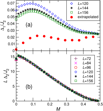
Figure 2: (Color online) Density matrix renormalization group results for the gaps at $J_{1}=-0.3\,J_{2}<0$ as a function of magnetization $M$. Panel (a) shows the single-spin excitation gap (16), panel (b) the finite-size gap (19) for two flipped spins multiplied by the chain length $L$.

In order to verify these field theory predictions, we perform complementary numerical computations using the DMRG method. white92 Open boundary conditions are imposed and we typically keep up to 400 DMRG states. From DMRG we obtain the ground-state energies $E(S^{z})$ as a function of total $S^{z}$. For those values of $S^{z}$ that emerge as a ground state in an external magnetic field we compute the single-spin excitation gap from

$$\Delta_{1}(M)=\frac{E(S^{z}+1)+E(S^{z}-1)-2\,E(S^{z})}{2}\,.$$ (16)

Fig. 2a shows numerical results for $\Delta_{1}$ at a selected value of $J_{1}=-0.3\,J_{2}<0$ for the largest system sizes investigated. We find that the finite-size behavior of the gap $\Delta_{1}(M,L)$ for system sizes $L\geq 24$ is well described by a $1/L$ correction. This will be further corroborated by field-theoretical arguments outlined below. Therefore, we extrapolate it to the thermodynamic limit using a fit to the form

$$\Delta_{1}(M,L)=\Delta_{1}(M)+\frac{a(M)}{L}+\cdots\,,$$ (17)

allowing for an additional $1/L^{2}$ correction for those values of $M$ where at least 4 different system sizes are available.

This extrapolation is represented by the full circles in Fig. 2a; errors are estimated not to exceed the size of the symbols. Our extrapolation for $\Delta_{1}$ is consistent with a vanishing gap at $M=0$ in agreement with previous numerical studies Itoi01 although bosonization predicts a non-zero – possibly very small – gap. Itoi01 ; Nersesyan98 ; Cabra98 The behavior of $\Delta_{1}(M)$ confirms the picture described above: the gap is non-zero for $M>0$, goes first through a maximum and then a minimum and finally approaches $\Delta_{1}/J_{2}\approx 0.023$ given by Eq. (15) for $M\to 1/2$.

We further wish to point out that for chains with periodic boundary conditions, the coefficient $a(M)$ of the finite-size extrapolation Eq. (17) is determined by the spin-wave velocity and the critical exponent of the soft mode from the $\Delta S^{z}=2$ channel. Indeed, using Eq. (8) where we can set $r=0$, and use the conformal mapping (12) to the cylinder, we see that the leading finite-size correction to the gap is:

$$\Delta_{1}(M,L)=\Delta_{1}(M)+\frac{1}{L}\frac{\pi v_{+}(M)}{4K_{+}(M)}\,.$$ (18)

Note that we have to replace sin with sinh in Eq. (12) in order to extract a gap, since we are dealing with Euclidean time. In addition we used the fact that in our approximation the effective Hamiltonian (5) is a direct sum of symmetric and antisymmetric sectors. Moreover, it is only the symmetric sector enjoying conformal invariance and consequently we perform the replacement $\tau\to\sinh\tau$ only in the symmetric sector. The antisymmetric sector has a spectral gap and its contribution to the finite-size corrections of the single-spin flip excitation energy are exponentially suppressed with system size.Tsvelick With this method one cannot fix the amplitudes of the $1/L^{2}$ term and beyond. Note furthermore that there may be additional surface terms for open boundary conditions as employed in the numerical DMRG computations. Nevertheless there is a dominant $1/L$ correction in any case.

Next, we briefly look at the $\Delta S^{z}=2$ excitations. Their finite-size gap is, in analogy to Eq. (16), computed with DMRG from

$$\Delta_{2}(M)=\frac{E(S^{z}+2)+E(S^{z}-2)-2\,E(S^{z})}{2}\,.$$ (19)

Fig. 2b shows numerical results for $L\,\Delta_{2}(M,L)$ again at the value $J_{1}=-0.3\,J_{2}<0$. One observes that the scaled finite-size gaps collapse onto a single curve which shows that $\Delta_{2}(M,L)$ scales linearly to zero with $1/L$, exactly as expected for gapless excitations in 1D. Furthermore, we observe that the scaled quantity $L\,\Delta_{2}(M,L)$ vanishes as one approaches saturation $M=1/2$ which indicates a vanishing of the velocity of the corresponding excitations at saturation.

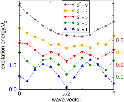
Figure 3: (Color online) Numerical dispersion spectrum in the subspaces of odd $S^{z}$ computed for $L=24$ and $J_{1}=-J_{2}<0$. The wave vector is given relative to the ground state wave vector (0 for $S^{z}=0,4,8$ and $\pi$ for $S^{z}=2,6$).

We proceed by discussing the wave-vector dependence of the $\Delta S^{z}=1$ excitation, while we remind the reader that the low-energy excitations are in the $\Delta S^{z}=2$ sector. Fig. 3 shows representative ED results obtained for rings with $L=24$ and $J_{1}=-J_{2}<0$. For ground states with low $S^{z}$, the $\Delta S^{z}=1$ excitation spectrum looks similar to the continuum of spinons. On the other hand, close to saturation one has single-magnon excitations with a minimum given by the classical value of the wave vector $k_{cl}=\arccos(|J_{1}|/4J_{2})$.Chubukov91 ; Cabra98 ; GMK98 We read off from Fig. 3 that upon lowering the magnetic field, this minimum shifts from the classical incommensurate value towards $\pi/2$, i.e. the value appropriate for two decoupled chains. This renormalization of the minimum of the magnon excitations towards the value of decoupled chains can be interpreted in terms of quantum fluctuations, which are enhanced when the density of magnons increases. A strong quantum renormalization of the pitch angle from its classical value at zero magnetization was previously observed by the coupled-cluster method and DMRG calculations.Bursill

V Summary

We have combined numerical techniques with analytical approaches and mapped out the ground state phase diagram of the frustrated ferromagnetic spin chain in an external magnetic field. We have established that with increasing magnetic field, the ground state crosses over from a spin-density-wave dominated to a nematic-like phase. Single spin flip excitations are gapped, giving rise to an exponential decay of in-plane spin correlation functions in both regimes. We have studied the single- and two-spin flip excitation energy numerically. Using tools from conformal field theory we have further shown that the amplitude of the leading $1/L$ correction term to the single-spin flip gap is determined by the critical exponent and the spin-wave velocity of the soft mode.

Finally, in order to apply our findings to the material LiCuVO₄, one should take into account interchain interactions as well as anisotropies, which are expected to be present in this system.Enderle05 At low fields, a helical state has been observed experimentally.Gibson04 ; Enderle05 On the other hand, for the purely one dimensional case, we have shown that upon increasing the magnetic field there is a competition between spin-density-wave and nematic-like tendencies. Those are the two leading instabilities at high magnetizations and thus they are the natural candidates to become long-range ordered in higher dimensions. The question whether there are true phase transitions at high fields in higher dimensions is beyond the scope of the current work.

- (1) M. Hase, H. Kuroe, K. Ozawa, O. Suzuki, H. Kitazawa, G. Kido, and T Sekine, Phys. Rev. B 70, 104426 (2004).
- (2) B. J. Gibson, R. K. Kremer, A. V. Prokofiev, W. Assmus and G. J. McIntyre, Physica B 350, e253 (2004).
- (3) M. Enderle, C. Mukherjee, B. Fåk, R. K. Kremer, J.-M. Broto, H. Rosner, S.-L. Drechsler, J. Richter, J. Malek, A. Prokofiev, W. Assmus, S. Pujol, J.-L. Raggazzoni, H. Rakoto, M. Rheinstädter, and H. M. Rønnow, Europhys. Lett. 70, 237 (2005).
- (4) M. G. Banks, F. Heidrich-Meisner, A. Honecker, H. Rakoto, J.-M. Broto, and R. K. Kremer, J. Phys.: Cond. Mat. 19, 145227 (2007).
- (5) N. Büttgen, H.-A. Krug von Nidda, L. E. Svistov, L. A. Prozorova, A. Prokofiev, and W. Aßmus, Phys. Rev. B 76, 014440 (2007).
- (6) S.-L. Drechsler, O. Volkova, A. N. Vasiliev, N. Tristan, J. Richter, M. Schmitt, H. Rosner, J. Málek, R. Klingeler, A. A. Zvyagin, and B. Büchner, Phys. Rev. Lett. 98, 077202 (2007).
- (7) H.-J. Mikeska and A. K. Kolezhuk, Lect. Notes Phys. 645, 1 (2004).
- (8) A. V. Chubukov, Phys. Rev. B 44, 4693 (1991).
- (9) F. Heidrich-Meisner, A. Honecker, and T. Vekua, Phys. Rev. B 74, 020403(R) (2006).
- (10) D. V. Dmitriev, V. Y. Krivnov, and J. Richter, Phys. Rev. B 75, 0114424 (2007).
- (11) R. O. Kuzian and S.-L. Drechsler, Phys. Rev. B 75, 024401 (2007).
- (12) See, e.g., T. Hikihara and A. Furusaki, Phys. Rev. B 69, 064427 (2004).
- (13) D. C. Cabra, A. Honecker, and P. Pujol, Eur. Phys. J. B 13, 55 (2000).
- (14) H. J. Schulz, Phys. Rev. B 34, 6372 (1986).
- (15) A. Läuchli, G. Schmid, and S. Trebst, Phys. Rev. B 74, 144426 (2006).
- (16) K. Totsuka, Phys. Lett. A 228, 103 (1997).
- (17) D. C. Cabra, A. Honecker, and P. Pujol, Phys. Rev. B 58, 6241 (1998).
- (18) V. E. Korepin, N. M. Bogoliubov, and A. G. Izergin, Quantum Inverse Scattering Method and Correlation Functions (Cambridge University Press, Cambridge, England, 1993).
- (19) S. Qin, M. Fabrizio, L. Yu, M. Oshikawa, and I. Affleck, Phys. Rev. B 56, 9766 (1997).
- (20) F. D. M. Haldane, Phys. Rev. Lett 47, 1840 (1981).
- (21) S. R. White, Phys. Rev. Lett. 69, 2863 (1992); Phys. Rev. B 48, 10345 (1993).
- (22) C. Itoi and S. Qin, Phys. Rev. B 63, 224423 (2001).
- (23) A. A. Nersesyan, A. O. Gogolin, and F. H. L. Eßler, Phys. Rev. Lett. 81, 910 (1998).
- (24) S. I. Matveenko and A. M. Tsvelik, private communication.
- (25) C. Gerhardt, K.-H. Mütter, and H. Kröger, Phys. Rev. B 57, 11504 (1998).
- (26) R. Bursill, G. A. Gehring, D. J. J. Farnell, J. B. Parkinson, T. Xiang, and C. Zeng, J. Phys. Cond. Mat. 7, 8605 (1995).