Circuit QED with a Flux Qubit Strongly Coupled
to a Coplanar Transmission Line Resonator

Abstract

We propose a scheme for circuit quantum electrodynamics with a superconducting flux-qubit coupled to a high-Q coplanar resonator. Assuming realistic circuit parameters we predict that it is possible to reach the strong coupling regime. Routes to metrological applications, such as single photon generation and quantum non-demolition measurements are discussed.

I Introduction

Until a few years ago it was an open question whether true quantum effects such as quantum entanglement would ever be observed in a man-made macroscopic electronic device. However, over the past decade, quantum coherence has been demonstrated in a variety of macroscopic systems, including superconducting circuits nakamura ; vanderwal ; chiorescu ; martinis2003 . Many of these experiments drew inspiration from the pioneering work on atomic qubits that took place a decade earlier Zeilinger99 . As the fields of atomic physics and quantum optics continue to advance, it makes sense to continue to look to them for guidance.

The universal nature of quantum mechanics is greatly to our advantage, in that the terminology and methodology apply as well to macroscopic as to microscopic systems. This allows well-known results from atomic physics and quantum optics to be used to plan and predict the outcome of experiments on solid state devices. Recently, such techniques have been applied with great success to implement a number of ideas such as quantum state tomography steffen , Mach-Zehnder interferometry oliver and sideband coolingvalenzuela .

This approach has also been very successful in the field of cavity quantum electrodynamics (CQED) [see Ref. gerry for an introduction]. In CQED an atomic 2-level system (i.e. a qubit) is made to interact with a high-finesse optical cavity with a coupling energy $\hbar g$. Provided that the relaxation rates $\gamma$ of the qubit and $\kappa$ of the cavity field are smaller than $g$ (known as the strong coupling criterion), it is possible to observe a coherent exchange of energy between the qubit and the cavity field. The resulting entangled states can be detected spectroscopically. Recently, Schoelkopf and co-workers wallraff ; blais achieved strong coupling in a macroscopic circuit comprising a superconducting charge qubit and a coplanar transmission line resonator. This new field is known as circuit-QED, and has many potential applications such as the generation and detection of single microwave photons. More recently strong coupling was observed in experiments on photonic crystals yoshie and quantum dotsreithmaier .

Much of the work to date on qubit-cavity systems has been focused on methods for making quantum non-demolition (QND) measurements of the qubit state. QND schemes have been used to read-out single qubits wallraff ; lupascu and also to measure the photon number in the cavity schuster . Several ways of reading out qubits using low-$Q$ cavities/resonators have also been reported Johanson ; ilichev , but these do not allow the strong coupling regime to be reached.

The benefits of superconducting circuit-QED systems over atomic systems are twofold. Firstly, the qubit energy can be tuned by varying the external magnetic field, enabling control over the qubit-cavity interaction. Secondly, qubit parameters such as the level separation at the degeneracy point can be engineered through appropriate circuit design. The main advantage of flux qubits over other types of superconducting qubits is that they are less susceptible to fluctuations in the background charge and the associated noise. This makes them less prone to decoherence, and therefore easier to manipulate in a deterministic way.

In section II we summarise the established background theory in the context of our proposed system; in III we show that it is possible to achieve strong coupling between a superconducting flux qubit Mooij-1999 and a high-Q coplanar transmission line resonator; in IV we present computer simulations of the resonator response; and in V we propose a scheme for producing single photons on demand.

II Theory of Circuit QED with a Flux Qubit

In this section we analyze the processes which occur when a superconducting qubit is coupled to a superconducting coplanar transmission line resonator, as shown in Fig. 1. The effect of coupling a flux qubit to a resonator has previously been experimentally demonstrated chiorescunature but the quality factor of the resonator was too small to fulfill the strong coupling criteria.

Two types of flux qubits will be discussed - an RF SQUID, which consists of a single Josephson junction in a superconducting loop, and a persistent current qubit (PCQ), which has three junctions in the loop, one of which is smaller than the others by a factor $\alpha$ Mooij-1999 . Both need to be biased by an external magnetic flux $\Phi_{x}$, which tunes the energy level separation through an anticrossing at $\Phi_{x}=0.5\Phi_{0}$. The resonator is a coplanar transmission line with inductance $L$ and capacitance $C$, which is weakly coupled to external transmission lines via coupling capacitors $C_{C}$.

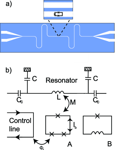
Figure 1: a) Sketch of a typical coplanar waveguide resonator of length l=$\lambda/2\approx 11$ mm. Shown is also how the qubit can be placed in between the centre conductor and the ground plane of the waveguide. b) Schematic diagram of a superconducting qubit coupled to a coplanar transmission line resonator. (A) Persistent current qubit. (B) RF SQUID. $M$ is the mutual inductance between the qubit and resonator, and $\Phi_{X}$ is the magnetic flux threading the qubit loop.

The Hamiltonian $H$ of the complete system is

$$H=H_{q}+H_{r}+H_{g}+H_{I}+H_{E}.$$ (1)

$H_{q}$ describes the qubit, $H_{r}$ the resonator, and $H_{g}$ the interaction between them. $H_{I}$ denotes the interaction of the system with a periodic drive field. Finally, $H_{E}$ describes the interaction of the resonator with its environment, resulting in the loss of photons to the external transmission lines and the interaction of the qubit with its environment, resulting in spontaneous decay from the excited state to the ground state.

The qubit Hamiltonian $H_{q}$ is given by the expression $(\hbar/2)(-\epsilon\sigma_{z}-\delta\sigma_{x})$ where $\sigma_{z}$ and $\sigma_{x}$ are Pauli spin matrices, $\delta$ is the the level repulsion, $\epsilon=(2I_{p}/\hbar)(\Phi_{x}-\Phi_{0}/2)$, and $I_{p}$ is the persistent current. In the case of an RF SQUID suitable for operation as a qubit, $I_{p}$ is roughly equal to half the critical current of the single junction, whereas, for the persistent current qubit, $I_{p}$ is approximately equal to the critical current of the smallest of the three junctions. If the qubit is operated at or near the degeneracy point, $H_{q}$ can be expressed more simply by transforming to the basis in which the ground state $|\downarrow\rangle$ and excited state $|\uparrow\rangle$ correspond to symmetric and antisymmetric superpositions of clockwise and anti-clockwise persistent currents. This yields

$$H_{q}=\frac{\hbar\omega_{0}}{2}(|\uparrow\rangle\langle\uparrow|-|\downarrow\rangle\langle\downarrow|)=\frac{\hbar\omega_{0}}{2}\sigma_{z},$$ (2)

where the level separation is $\hbar\omega_{0}$, $\omega_{0}$ being the qubit Larmor frequency $\sqrt{\epsilon^{2}+\delta^{2}}$.

Assuming the resonator supports only a single mode of the electromagnetic field, its Hamiltonian is given by

$$H_{r}=\hbar\omega_{r}\left(a^{\dagger}a+\frac{1}{2}\right),$$ (3)

where $a^{\dagger}$($a$) is the creation(annihilation) operator which creates (destroys) a single photon in the cavity. The eigenstates of the resonator described by this Hamiltonian are Fock states $|0\rangle\ldots|n\rangle\ldots$ with $n$ photons. The single mode condition corresponds to a harmonic oscillator with the energy levels at $\hbar\omega_{r}(n+1/2)$ and the zero-point energy $\hbar\omega_{r}/2$.

The interaction between the radiation and the qubit is described as the dipole interaction $H_{g}=-\mathbf{\hat{\mu}\cdot\hat{B}}$ between a magnetic moment $\mathbf{\mu}$ of the persistent current circulating in the qubit loop and the magnetic field $\mathbf{B}$ in the resonator. Introducing quantization, this term in the Hamiltonian can be written in the form

$$H_{g}=\hbar g(a^{\dagger}\sigma^{-}+\sigma^{+}a),$$ (4)

where $\sigma^{+}$($\sigma^{-}$) is the raising(lowering) operator for the qubit. This expression is valid in the so-called non-dispersive regime where $\omega_{r}\approx\omega_{0}$ . The constant $g$ characterizes the qubit-photon interaction strength and the expression in the brackets describes the process whereby the qubit can be excited by absorbing a photon, or a photon can be generated at the expense of de-exciting the qubit into its ground state. In the next section we shall explicitly calculate the dipole coupling strength $g$ for specific designs of the qubit and the cavity.

The interaction of the coupled system with an external classical drive field can be seen as a periodic exchange of photons between the resonator and the driving field:

$$H_{I}=\xi(e^{-i\omega t}a^{\dagger}+e^{i\omega t}a),$$ (5)

where $\xi$ is the drive amplitude. One can also drive the qubit directly using a separate control line leading to terms $\xi^{\prime}(e^{-i\omega t}\sigma^{+}+e^{i\omega t}\sigma^{-})$, but we shall not consider this case any further.

Adding the terms (2)-(5) together we arrive at the driven Jaynes-Cummings Hamiltonian wallsandmilburn

$$H=\frac{\hbar\omega_{0}}{2}\sigma_{z}+\hbar\omega_{r}\left(a^{\dagger}a+\frac{1}{2}\right)+\hbar g(a^{\dagger}\sigma^{-}+\sigma^{+}a)$$ (6)

$$+\>\xi(e^{-i\omega t}a^{\dagger}+e^{i\omega t}a).$$

This Hamiltonian can be used to write down a master equation which completely describes the dynamics of the system. All the parameters which define the system can be conveniently written in units of angular frequency – a convention which we will follow here. If the cavity is weakly coupled to an already weak drive field one can achieve a regime when only two lower Fock states of the resonator are relevant. Within the picture described above we make one two-level system, the qubit, interact with another two-level system, the resonator. When the qubit is detuned from the resonator the eigenstates of the coupled system can be written: $|0\downarrow\rangle$, $|0\uparrow\rangle$, $|1\downarrow\rangle$ and $|1\uparrow\rangle$, where the number represents a Fock state of the resonator and the arrow represents the qubit state. However, when the qubit is brought into resonance, $H_{g}$ couples the states $|0\uparrow\rangle$ and $|1\downarrow\rangle$ and lifts their degeneracy. The system will oscillate between the states $|0\uparrow\rangle$ and $|1\downarrow\rangle$ at a frequency $\Omega=2g$ , known as the vacuum Rabi frequency semba , giving rise to a splitting alsing of the central peak as shown in Fig. 2. One can visualize this as a cycle in which the resonator and qubit continuously exchange an amount of energy equal to one photon. As the drive amplitude increases it will start to perturb the system. This leads to a set of states that are shifted by

$$E_{n}=\pm\sqrt{n}\hbar g[1-(2\xi/g)^{2}]^{3/4}.$$ (7)

Hence, the effect of the drive is to reduce the Rabi frequency.

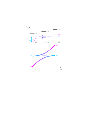
Figure 2: Energy levels of the coupled qubit-cavity system. On the left of the diagram the qubit is far detuned from the cavity. As we move from left to right, the magnetic flux threading the qubit loop is increased, tuning the qubit transition frequency into resonance with the cavity. On the right of the diagram, the qubit is once again far detuned.

The coupling strength $g$ can be determined experimentally by making a spectroscopic measurement of the splitting $\Delta E_{1}$. The drive amplitude should be reduced until the splitting reaches its maximum value, where it is equal to $2g\hbar$.

The above discussion covers the resonant regime, where the qubit is tuned into resonance with the cavity. In contrast, when the detuning $\Delta=\omega_{0}-\omega_{r}$ is large, such that $g/\Delta\ll 1$, a dispersive Stark shift pulls the cavity frequency by $\pm g^{2}/\Delta$. This so-called dispersive regime can be used to perform quantum non-demolition measurements of the qubit state blais .

The effects of the environment on the system are taken into account by the term $H_{E}$. There are three types of damping that need to be considered:

• Photons leak out of the cavity at a rate $\kappa=\omega_{r}/Q$, where Q is the cavity quality factor.

• The qubit relaxes at a rate $\gamma=1/T_{1}$, where $T_{1}$ is the energy relaxation time.

• Pure dephasing of the qubit at a rate $\gamma_{\phi}=1/T_{\phi}=1/T_{2}-2/T_{1}$, where $T_{2}$ is the dephasing time.

Dephasing plays a larger role in solid state systems than atomic systems, due to the stronger interaction of solid state qubits with their environments. In the absence of pure dephasing we would have $T_{2}=2T_{1}$ but in real systems $T_{2}$ is frequently much shorter than that, indicating the need to take pure dephasing into account.

III Strong Coupling with a Flux Qubit

Below we estimate the coupling strength $g$ using a semi-classical approach. We treat the flux qubit as a magnetic dipole and assume that it is placed at a magnetic field antinode of the resonator. The coupling strength is given by $g=\mu B_{0rms}/\hbar$, where $B_{0rms}$ is the zero-point root mean square magnetic field generated by the current fluctuations at the antinode of the resonator. The magnetic dipole moment of the qubit is given by $\mu=I_{p}A$, where $I_{p}$ is the persistent current flowing around the loop and $A$ is the loop area. We can estimate $B_{0rms}$ by considering the zero point energy of the resonator, $\hbar\omega_{r}/2$. This energy cycles continuously between inductive and capacitive components. The magnetic field is determined by the inductive component, $LI(t)^{2}/2$, where $L$ is the total equivalent inductance of the resonator near resonance and $I(t)$ is the instantaneous current. At the moment when the energy is purely inductive, we have $(1/2)LI_{max}^{2}=(1/2)\hbar\omega_{r}$. Since I(t) undergoes sinusoidal oscillation we therefore have that

$$I_{rms}=\sqrt{\frac{\hbar\omega_{r}}{2L}}.$$ (8)

Assuming that current flows in thin strips (whose width is determined by the superconducting penetration depth) at the edges of the centre conductor and ground plane, the field at the antinode of the fundamental mode is approximately given by

$$B_{0rms}\approx\frac{\mu_{0}I_{rms}}{\pi r},$$ (9)

where $\mu_{0}$ is the permeability of free space and $r$ is half the width of the gap between the centre conductor and the ground plane (we assume the qubit is placed at the centre of the gap). Therefore, the coupling strength between the qubit and resonator is given approximately by

$$g\approx\frac{I_{p}A\mu_{0}}{\hbar\pi r}\sqrt{\frac{\hbar\omega_{r}}{2L}}.$$ (10)

By inserting realistic values for the parameters in the above equation we can obtain an estimate of $g$.

First, we choose the fundamental frequency of the resonator. It is convenient to choose a value that lies within the range 4–8 GHz, as this is well within the design scope of both the qubit and resonator, and can be accessed with commercial microwave sources and components. We choose $\omega_{r}/2\pi=6$ GHz. With a centre conductor of width $\sim 10$ $\mu$m and a gap of width $\sim 5$  $\mu$m, it is possible to achieve a total inductance $L\sim 2$ nH for a resonator operated at its fundamental frequency..

Next, we choose $I_{p}$ such that the transition frequency $\omega_{0}$ of the qubit at the degeneracy point is slightly less than that of the resonator. This will enable us to tune the qubit in and out of resonance with the resonator by changing the external flux $\Phi_{x}$ threading the qubit loop. For the 3-junction persistent current qubit having two junctions of critical current $I_{c}=800$ nA and junction capacitance $C=4$ fF, and one junction of critical current $\alpha I_{c}$, where $\alpha=0.72$, we get $\omega_{0}/2\pi=4.9$ GHz at the degeneracy point and $I_{p}\approx 580$ nA. These parameters were obtained by solving the Schroedinger equation numerically. The transition frequency $\omega_{0}$ does not depend on the area $A$ of the qubit loop, provided that the loop inductance remains small compared with the Josephson inductance. However, we note that the larger the loop area, the greater the (undesired) coupling to the environment. Here we choose a value $A\approx 8$ $\mu$m².

With the above parameters we obtain $g/2\pi\approx 35$ MHz. We now compare this with the rate of photon loss from the resonator $\kappa$ and the relaxation rate of the qubit $\gamma$. When $g>\kappa,\gamma$, the coupled system is able to undergo many cycles ($\approx 2g/(\kappa+\gamma)$) of vacuum Rabi oscillation before losing coherence. This is important for applications such as single microwave photon generation. The photon loss rate from the resonator is given by $\kappa/2\pi=\omega_{r}/Q$, where $Q$ is the loaded quality factor of the resonator. It is possible to design a resonator with $Q=10^{5}$, yielding $\kappa/2\pi\approx 0.1$ MHz. The relaxation rate of the qubit is given by $\gamma=2\pi/T_{1}$. Taking $T_{1}\sim 1$ $\mu$s chiorescu , we obtain $\gamma/2\pi\approx 1$ MHz. Naturally, the values for $T_{1}$ and $T_{2}$ for a real system can not be predicted with any accuracy and will depend on the experimental conditions. However, based on the data available in the literature bertet ; kakuyanagi we believe that the aforementioned values are reasonable. Hence, it is clear that our estimated value of $g$ for the persistent current qubit should satisfy the strong coupling criterion.

For an RF SQUID with critical current $I_{c}=10$ $\mu$A, area $A=64$ $\mu$m², loop inductance $L_{SQUID}=35$ pH and junction capacitance $C=50$ fF, we obtain a transition frequency $\omega_{0}/2\pi=4.6$ GHz. In contrast to the persistent current qubit, the area of the RF SQUID does affect the transition frequency, via the loop inductance. It is difficult to reduce the area further than the value we have chosen, as this necessitates increasing the critical current and decreasing the junction capacitance, which becomes increasingly difficult to achieve in practice. Close to the degeneracy point, the persistent current $I_{p}$ in the above SQUID is expected to be about 5 $\mu$A. Combined with the increased loop area, this is likely to lead to an even larger coupling strength $g$ than predicted for the persistent current qubit (unless the SQUID is displaced significantly from the antinode of the resonator) but at the same time make qubit more susceptible to noise. The fact that the loop area of the 3-junction persistent current qubit can be made small enough to render it relatively insensitive to flux noise is one reason why it has been so successfully used by e.g Mooij and co-workers Mooij-1999 ; chiorescu .

IV Numerical simulation of the spectrum under microwave excitation

Having shown that it is possible to reach the strong coupling regime with a flux qubit coupled to a coplanar resonator, we now simulate the results of a spectroscopic experiment to measure $g$. The experiment would involve driving the coupled system with an external microwave field whose frequency $\omega_{l}$ would be swept through the resonance of the coupled system. The most straightforward way to probe the response of the system would be to use what effectively amounts to a standard microwave transmission ( S₁₂ ) measurement of the cavity. The experiment would be done by starting with the qubit far detuned from the resonator, then stepping the external magnetic flux to tune the qubit through the cavity resonance. This type of experiment would allow us to record the output power of the resonator as a function of qubit Larmor frequency.

These simulations were performed by solving the master equation using a Liouvillian with the Hamiltonian (II) and three collapse (Lindblad) operators which account for the decay and dephasing of the qubit and the cavity at the aforementioned rates $\kappa$,$\gamma$ and $\gamma_{\phi}$ (i.e. the effects of $H_{E}$). A brief description of the formalism can be found in appendix B. All simulations were performed using the “Quantum Optics Toolbox” developed by TanTan . Note that all the figures show the spectrum of the intracavity field (see appendix C for the definition and a description of how it is calculated).

In the regime where the qubit Larmor frequency $\omega_{0}$ is very far detuned from the cavity (i.e. when even dispersive effects are negligible) the qubit and the cavity are effectively decoupled and no exchange of energy can take place. If the system is probed by measuring the response of the cavity, a single peak located at the bare resonance frequency $\omega_{r}$ will be seen.

If instead the qubit is tuned exactly on resonance ($\Delta=0$) the effects of the coupling become clearly visible. Now, there are two peaks located at $\omega_{r}\pm\Omega/2=\omega_{r}\pm g$ as can be seen in fig. 3.

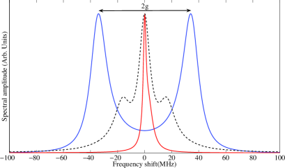
Figure 3: The spectrum far from resonance (where the only effect of the qubit is to broaden the resonance) and at zero de-tuning for small drive (mean steady-state photon number $\langle n\rangle<10^{-3}$), the latter giving rise to a Rabi splitting $2g$. Shown is also the spectrum at large ($\langle n\rangle\approx 8$) drive amplitudes (dashed line).

.

In between these two extremes there is a gradual change from a single- to a double-peaked spectrum where the splitting is approximately $g^{2}/\Delta$ as can be seen in the left picture of fig. 4. In this case the pure dephasing rate $\gamma_{\phi}$ was set to zero. The result is a ”diamond-shaped” picture with a maximum splitting of $2g$ at zero detuning.

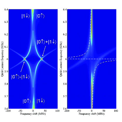
Figure 4: (Color online) Power spectrum of the coupled qubit-resonator system as a function of qubit detuning in the strong coupling limit. The frequency of the drive field $\omega_{l}$ is held at the resonance frequency $\omega_{r}$ of the bare resonator, while the Larmor frequency $\omega_{0}$ of the qubit is tuned by changing the external magnetic field. Left: Spectrum in the absence of pure dephasing. Right: Adding a pure dephasing channel to the dissipation results in an asymmetric spectrum, here the pure dephasing rate $\gamma_{\phi}$ is 9.5 MHz. Shown is also one branch of the expression $\pm g^{2}/\Delta$ (white dashed line). The following parameters were used in the simulations (in GHz): $\omega_{r}=\omega_{l}=6$, $g=0.035$, $\kappa=0.004$, $\gamma=0.001$ and $\xi/\hbar=0.25\kappa$.

Far from resonance we can identify the four branches as being associated with the states $|0\uparrow\rangle$ and $|1\downarrow\rangle$ above and below the resonance. Exactly on resonance the system is in a superposition of states $|0\uparrow\rangle\pm|1\downarrow\rangle$. This is in agreement with the diagram shown in fig. 2. Note that e.g. an interferometric measurement method Oxborrow-2005 must be used in order to be able to observe the whole spectrum, a simpler transmission experiments would only see one peak off-resonance since such a measurement only records transitions between photon states where the final state can emit a photon; in this case $|0\uparrow\rangle\leftrightarrow|1\downarrow\rangle$.

The right picture in fig. 4 shows the spectrum when pure dephasing is introduced to the model. The result is somewhat more complicated in that the spectral weights are asymmetric with respect to $w_{r}-w_{l}=0$ when the qubit is detuned from resonance. The reason for this is that dephasing leads to a loss of coherence, meaning that the qubit tends to stay in its ground state and the coupling between the states $|0\uparrow\rangle$ and $|1\downarrow\rangle$ is reduced, the system is therefore no longer in a superposition of those states. Whence, states with zero photons in the cavity are effectively ”decoupled” from the one-photon states. Since only states which allow for (at least) one photon in the cavity can be measured it follows that only the two branches (one above and one below resonance) that (approximately) correspond to $\pm|1\downarrow\rangle$ will be clearly visible. Note, however, that despite the loss of coherence an on-resonance measurement would still show two peaks separated by $2g$, i.e. exactly on resonance this situation is effectively indistinguishable from the more coherent case even when the full spectrum is measured.

While there are no bound states in the limit of strong driving $\xi>g/2$ a continuum of states still exists giving rise to complex spectra (dashed line in fig. 3). The structure is reminiscent to the so-called ”Mollow” peaks, well known in atomic physics from e.g. fluorescence spectroscopy. However, in the latter case the peaks are the result of strong driving of the atom (qubit) whereas in this simulation the cavity is being driven so the similarity is somewhat superficial. When as in this case the cavity is driven so strongly that there are on average several photons in the cavity, we see both a drive induced shift of the position of the sidebands and a reappearance of the central peak. Note that since it is difficult to directly relate the parameter $\xi$ to the power output from a microwave generator, care must be taken not to drive the system inadvertently into this regime.

For the persistent current qubit considered here, a detuning of $\pm 0.4$ GHz corresponds to an external magnetic flux in the range $\pm 10^{-4}\Phi_{0}$ which is a useful value for a real experiment. However, for the RF SQUID, the flux required is rather less: $\pm 3\cdot 10^{-5}\Phi_{0}$.

One effect which is not taken into account in our simulations is the presence of thermal photons in the cavity. Thermal effects can, in general, be neglected when working with optical cavities due to the very small average number of photons at those frequencies. In experiment on solid state qubits this is, however, not generally true since they are operated in the microwave range. Also, the relevant temperature scale is set not only by the the phonon temperature (e.g. the temperature of the mixing chamber of a dilution refrigerator) but also by the amount of noise (essentially ”hot” photons) which reaches the system via the leads. However, in a well-filtered system a total temperature of 50 mK is attainable. The resonator will then nearly be in its ground state with an average thermal occupancy $\bar{n}$ of 0.009 and thermal fluctuations in the photon number of the order of 0.1. This justifies ignoring thermal effects in our simulations for now. That said, even a moderate increase in temperature can significantly change the outcome of an experiment rau . One further simplifying assumption in the model is that $T_{1}$ and $T_{2}$ do not change as the qubit is detuned from the optimal bias point $\Phi_{0}/2$. While this is clearly unrealistic, it has been experimentally shown kakuyanagi that neither parameter should change dramatically in the parameter range considered here, giving some justification to this approximation.

V Applications of circuit-QED

One of the most important applications of circuit QED is the generation of single microwave photons on demand. Single photon sources in the optical regime have been realized using e.g. cavity QED with atoms and high finesse optical cavities Oxborrow-2005 . Design and fabrication of deterministic sources that operate in the microwave regime have proved to be more difficult, but a source based on superconducting circuit-QED was recently demonstrated houck . This kind of source could be used for quantum radiometry, as well as for quantum information applications such as quantum key distribution.

Various schemes can be envisaged mariantoni ; marquardt ; zagoskin ; saito , by which single photons can be generated with a circuit QED device. Below, we describe a straightforward technique, based on manipulation of the qubit state with microwave pulses and rapid changes in the DC magnetic field to tune the qubit in and out of resonance with the cavity.

Our technique begins with the qubit far detuned from the cavity and the combined system in its ground state $|0\downarrow\rangle$. A microwave $\pi$-pulse is applied to the qubit to excite it to the state $|0\uparrow\rangle$ [Fig. 5(a)], and this is followed by a step in the magnetic field to bring the qubit into resonance with the cavity [Fig. 5(b)]. The state of the system immediately after the step is still $|0\uparrow\rangle$, but due to the qubit-cavity interaction on resonance, this is no longer an eigenstate, so the system begins to precess around the equator of the Bloch sphere at the vacuum Rabi frequency $2g$. After a time $2\pi/4g$, the state of the system will be $|1\downarrow\rangle$ [Fig. 5(c)]. This means that coherent energy exchange has taken place between the qubit and the cavity, creating a photon-like state. Another step in magnetic field detunes the qubit from the cavity so that the state $|1\downarrow\rangle$ is once more an eigenstate of the system [Fig. 5(d)]. The system remains in this state until the photon decays out of the cavity into one of the external waveguides in a time of order $2\pi/\kappa$. By repeating this sequence many times, photons can be generated on demand, provided that the time window within which they are required is much longer than $2\pi/\kappa$.

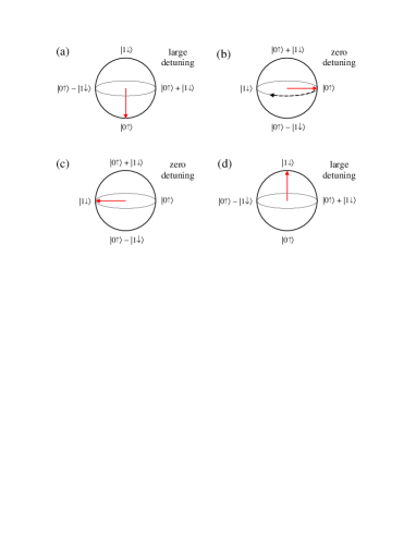
Figure 5: (Color online). Bloch sphere diagrams showing the state of the qubit-cavity system at successive stages of the single photon generation process.

If a scheme similar to the one above is implemented, it is important to prove that it generates single photons deterministically, rather than stochastically. At optical frequencies this is done by studying photon-counting statistics using interferometric measurements. Such measurements require the use of a beamsplitter. An analogous experiment can be envisaged in the microwave regime, provided that a microwave beamsplitter can be realised. Such a device has been proposed recently mariantoni , and could lead to a microwave analogue of the Hanbury-Brown and Twiss interferometer Oxborrow-2005 .

VI Conclusions

We have shown that it should be possible to reach the strong coupling regime using a flux qubit coupled to a coplanar waveguide resonator. If realized, it would open the door to potential applications in metrology, quantum communication and experimental tests of quantum mechanics. The fact that conventional lithography can be used to fabricate the samples and that the experimental parameters can be chosen freely can in some cases a be significant advantage compared to CQED implentantaions utilizing e.g. atoms of ions. Since the relevant frequencies are in the microwave regime it is also possible to use well established methods to manipulate the system. The main drawback compared to experiments done at optical frequencies is the short coherence time of the qubit and the fact that the system must be operated at very low temperatures.

VII Acknowledgments

The authors would like to thank Mark Oxborrow, Alexandre Zagoskin, Alexander Blais and Vladimir Antonov for helpful discussions and comments. We would also like to thank Scott Parkins for his help with the Quantum Optics Toolbox. This work was funded by the UK Department of Trade and Industry Quantum Metrology Programme, project QM04.3.4. and the Swedish Research Council.

Appendix A Derivation of the Hamiltonian

It is useful to compare the informal procedure used in the introduction of this paper to derive the Hamiltonian with a more formal approach. Starting with the bare qubit Hamiltonian $-\frac{1}{2}(\epsilon\sigma_{z}+\Delta\sigma_{x})$ where $\epsilon=2I_{p}(\Phi_{x}-\Phi_{0}/2)$ we proceed just as before by noting that the flux threading the qubit loop will be modulated via the mutual inductance $M$ that couple the fluctuations in the cavity to the qubit. Writing the total external flux as $\Phi_{x}=\Phi_{x}^{DC}+\delta\Phi$, where $\delta\Phi=M\sqrt{\frac{\hbar\omega_{r}}{2L}}(a^{\dagger}+a)$, adding the Hamiltonian for the oscillator mode and the external field and finally transforming into the eigenbasis of the qubit we get

$$H= \hbar\omega_{r}\left(a^{\dagger}a+\frac{1}{2}\right)+\frac{\hbar\omega_{0}}{2}\sigma_{z}+\hbar g(a^{\dagger}\sigma_{-}+\sigma_{+}a)\sin\theta$$ (11)

$$+\xi(e^{-i\omega t}a^{\dagger}+e^{i\omega t}a)-\hbar g(a^{\dagger}+a)\sigma_{z}\cos\theta$$

in the RWA. Here we have introduced the mixing angle $\theta=\arctan{\Delta/\epsilon}$. This Hamiltonian is identical to the J-C Hamiltonian (II) except that we now have an effective coupling $g\sin\theta$ and an extra term $\hbar g(a^{\dagger}+a)\sigma_{z}\cos\theta$ which is zero when the qubit is operated at the degeneracy point $\theta=\pi/2$. By moving to an interaction frame rotating at the drive frequency $\omega$ we see that all terms in the Hamiltonian (11) are time-independent except the last term which picks up a factor $\exp(-iw\omega)$, meaning it can be neglected in the rotating wave approxiamtion. Note, however, that this additional term can potentially play a role in the dispersive regime.

Appendix B Dissipation

The effects of the environment on a quantum system is in general very difficult to model but is nevertheless crucial to understand since it is the cause of decoherence. However, assuming the interaction with the environment is Markovian the evolution of the (reduced) density matrix of the system can be described by a master equation $\dot{\rho}=\mathbf{L}\rho$ of Lindblad form breuer

$$\frac{\partial\rho}{\partial t}=-\frac{i}{\hbar}[H,\rho]+\sum^{3}_{k=1}\left(C_{k}\rho C_{k}^{\dagger}-\frac{1}{2}\left(C_{k}^{\dagger}C_{k}\rho+\rho C_{k}^{\dagger}C_{k}\right)\right)$$ (12)

where $C_{k}$ are Lindblad operators. In the case considered here we have 3 Lindblad operators. Firstly, the relaxation from the excited state to the ground state at a rate $\gamma_{1}=1/T_{1}$ represented by a Lindblad operator proportional to the lowering operator $\hat{\sigma}^{-}$, i.e. $C_{1}=\sqrt{\gamma_{1}}\hat{\sigma}^{-}$. The cavity is loosing energy at a rate $\kappa=\omega_{r}/Q$ which leads to the ”destruction” of photons in the system, $C_{2}=\sqrt{\kappa}a$. Finally, we also need to consider pure dephasing of the qubit at a rate $\gamma_{\phi}=1/T_{\phi}=1/T_{2}-1/2T_{1}$ where $T_{2}$ is the usual total dephasing time of the qubit. This process is represented by the operator $C_{3}=\sqrt{\frac{\gamma_{\phi}}{2}}\hat{\sigma}_{z}$.

Appendix C Calculation of the spectrum

Our aim is to calculate the steady-state power spectrum $S(\omega)$ of the intracavity field, formally this is defined in terms of the photocount output from the cavity as seen by a monochromatic detector wallsandmilburn . The spectrum can be calculated from the 2-time correlation function glauber $\langle a^{\dagger}(t+\tau)a(\tau)\rangle$

$$S(\omega)=\frac{1}{2\pi}\int_{-\infty}^{\infty}e^{-i\omega\tau}\langle a^{\dagger}(\tau+t)a(t)\rangle d\tau$$ (13)

which can be evaluated using the quantum-regression theorem

$$<a^{\dagger}(\tau+t)a(t)>=\mathrm{Tr}\{a^{\dagger}e^{\mathbf{L}\tau}a\rho\}$$ (14)

where the Liovillian (which includes the three Lindblad operators defined in Appendix B) is given by the right hand side of equation 12 and $\rho$ is the steady-state density matrix which is the solution to $\mathbf{L}\rho=0$ These calculations are straightforward using the built-in routines of the ”Quantum Optics Toolbox”.

References

- [1] Y. Nakamura, Yu.A. Pashkin, and J.S. Tsai. Coherent control of macroscopic quantum states in a single-cooper-pair box. Nature, 398:786–8, 1999.
- [2] C.H. Van Der Wal, A.C.J. Ter Haar, F.K. Wilhelm, R.N. Schouten, C.J.P.M. Harmans, T.P. Orlando, S. Lloyd, and J.E. Mooij. Quantum superposition of macroscopic persistent-current states. Science, 290:773–7, 2000.
- [3] I. Chiorescu, Y. Nakamura, C.J.P.M. Harmans, and J.E. Mooij. Coherent quantum dynamics of a superconducting flux qubit. Science, 299:1869–71, 2003.
- [4] J.M. Martinis, S. Nam, J. Aumentado, and C. Urbina. Rabi oscillations in a large Josephson-junction qubit. Phys. Rev. Lett., 89(11):117901–1, 2003.
- [5] A. Zeilinger. Experiment and the foundations of quantum physics. Reviews of Modern Physics, 71:288, 1999.
- [6] Matthias Steffen, M. Ansmann, Radoslaw C. A ND Bialczak, N. Katz, Erik Lucero, R. McDermott, Matthew Neeley, E. M. Weig, A. N. Cleland, and John M. Martinis. Measurement of the entanglement of two superconducting qubits vis quantum state tomography. Science, 313:1423–1425, 2006.
- [7] William D. Oliver, Yang Yu, Janice C. Lee, Karl K. Berggren, Leonid S. Levitov, and Terry P. Orlando. Mach-Zehnder interferometry in a strongly driven superconducting qubit. Science, 310:1653–1657, 2005.
- [8] S.A Valenzuela, W. Oliver, D.M. Berns, K.K. Berggren, L.S. Levitov, and T.P. Orlando. Microwave-induced cooling of a superconducting qubit. Science, 314:1589–1591, 2006.
- [9] C.S. Gerry and P.L. Knight. Introductory Quantum Optics. Cambridge University Press, 2005.
- [10] A. Wallraff, D. I. Schuster, A. Blais, L. Frunzio, R.-S. Huang, J. Majer, S. Kumar, S. M. Girvin, and R. J. Schoelkopf. Strong coupling of a single photon to a superconducting qubit using circuit quantum electrodynamics. Nature, 431:162–167, 2004.
- [11] A Blais, R Huang, A Wallraff, S.M. Girvin, and R.J. Shoelkopf. Cavity quantum electrodynamics for superconducting electrical circuits: An architecture for quantum computation. Phys. Rev. A, 69:062320, 2004.
- [12] T Yoshie, A. Sherer, A. Hendrickson, G. Khitrova, H.M. Gibbs, G. Rupper, C. Ell, O.B. Shchekin, and D.G. Deppe. Vacuum Rabi splitting with a single quantum dot in a photonic crystal nanocavity. Nature, 432:200–203, 2004.
- [13] J. P. Reithmaier, A. L ffler, G. Sk, C. Hofmann, S. Kuhn, S. Reitzenstein, L.V. Keldysh, V.D. Kulakovskii, Reinecke T. L., and A. Forchel. Strong coupling in a single quantum dot-semiconductor microcavity system. Nature, 432:197–200, 2004.
- [14] A. Lupaşcu, S. Saito, T. Pictot, P.C. de Groot, C.J.M. Harmans, and J.E. Mooij. Quantum non-demolition measurement of superconducting two-level system. arXiv:cond-Mat, (0611505), 2006.
- [15] D. I. Schuster, A. A. Houck, J. A. Schreier, A. Wallraff, J. M. Gambetta, A. Blais, L. Frunzio, B. Johnson, M. H. Devoret, S. M. Girvin, and Schoelkopf R. J. Resolving photon number states in a superconducting circuit. Nature, 445:515, 2007.
- [16] G. Johansson, L. Tornberg, and C. M. Wilson. Fast quantum limited readout of a superconducting qubit using a slow oscillator. Phys. Rev. B, 74:100504R, 2006.
- [17] Grajcar et al. Four-qubit device with mixed couplings. Phys. Rev. Lett., 96:047006, 2006.
- [18] J. E. Mooij, T. P. Orlando, L. Levitov, L. Tian, C. H. van der Wal, and S. Lloyd. Josephson persistent-current qubit. Science, 285:1036, 1999.
- [19] I. Chiorescu, P. Bertet, K. Semba, Y. Nakamura, C.J.P.M. Harmans, and J.E. Mooij. Coherent dynamics of a flux qubit coupled to a harmonic oscillator. Nature, 431:159–162, 2004.
- [20] D.F. Walls and G.J. Milburn. Quantum Optics. Springer-Verlag, 1994.
- [21] J. Johansson, S. Saito, T. Meno, H. Nakano, M. Ueda, K. Semba, and H. Takayanagi. Vacuum Rabi oscillations in a macroscopic superconducting qubit LC oscillator system. Physical Review Letters, 96:127006, 2007.
- [22] P. Alsing, D.S Guo, and H.J. Carmichael. Dynamic Stark effect for the Jaynes-Cummings system. Phys. Rev. A, 47(7):5135–5143, 1994.
- [23] P. Bertet, I. Chiorescu, G. Burkard, K. Semba, C. J. P. M. Harmans, D.P. DiVincenzo, and J. E. Mooij. Relaxation and dephasing in a flux qubit. arXiv:cond-mat, (0412485), 2004.
- [24] K. Kakuyanagi, T. Meno, S. Saito, H. Nakano, K. Semba, H. Takayanagi, F. Deppe, and A. Shnirman. Dephasing of a superconducting flux qubit. Physical Review Letters, 98:47004, 2007.
- [25] S. Tan. A computational toolbox for quantum and atomic optics. Journal of Optics B, 1:424–432, 1999.
- [26] M. Oxborrow and A. Sinclair. Single photon sources. Contemporary Physics, 46(3):173–206, 2005.
- [27] I Rau, G. Johansson, and A. Shnirman. Cavity quantum electrodynamics in superconducting circuits: Susceptibility at elevated temperatures. Phys. Rev. B, 70:054521, 2004.
- [28] A. A. Houck, D. I. Schuster, J. M. Gambetta, J. A. Schreier, B. R. Johnson, J. M. Chow, J. Majer, L. Frunzio, M. H. Devoret, S. M. Girvin, and R. J. Schoelkopf. Generating single microwave photons in a circuit. arXiv:cond-mat, (0702648v1), 2007.
- [29] M. Mariantoni, M.J. Storcz, F.K. Wilhelm, W.D. Oliver, A. Emmert, A. Marx, R. Gross, H. Christ, and E. Solano. On-chip microwave Fock states and quantum homodyne measurements. arXiv:Cond-Mat, (0509737), 2006.
- [30] F. Marquardt. Efficient on-chip source of microwave photon pairs in superconducting circuit qed. arXiv:cond-Mat, (0605232), 2006.
- [31] A.M. Zagoskin, M. Grajcar, and A.N. Omelyanchouk. Selective amplification of a quantum state. Phys. Rev. B, 70:060301(R), 2004.
- [32] K. Saito, M. Wubs, S. Kohler, P. Hänggi, and Y. Kayanuma. Quantum state preparation in circuit QED via Landau-Zener tunneling. Europhysics Letters (EPL), 76(1):22–28, 2006.
- [33] H. P. Breuer and F. Petruccione. The theory of open quantum systems. Oxford University Press, 2004.
- [34] R. J. Glauber. Coherent and incoherent states of radiation field. Physical Review, 131:2766–2788, 1963.