Limit distributions and scaling functions

Abstract

We discuss the asymptotic behaviour of models of lattice polygons, mainly on the square lattice. In particular, we focus on limiting area laws in the uniform perimeter ensemble where, for fixed perimeter, each polygon of a given area occurs with the same probability. We relate limit distributions to the scaling behaviour of the associated perimeter and area generating functions, thereby providing a geometric interpretation of scaling functions. To a major extent, this article is a pedagogic review of known results.

1 Introduction

For a given combinatorial class of objects, such as polygons or polyhedra, the most basic question concerns the number of objects of a given size (always assumed to be finite), or an asymptotic estimate thereof. Informally stated, in this overview we will analyse the refined question:

What does a typical object look like?

In contrast to the combinatorial question about the number of objects of a given size, the latter question is of a probabilistic nature. For counting parameters in addition to object size, one asks for their (asymptotic) probability law. To give this question a meaning, an underlying ensemble has to be specified. The simplest choice is the uniform ensemble, where each object of a given size occurs with equal probability.

For self-avoiding polygons on the square lattice, size may be the number of edges of the polygon, and an additional counting parameter may be the area enclosed by the polygon. We will call this ensemble the fixed perimeter ensemble. For the uniform fixed perimeter ensemble, one assumes that, for a fixed number of edges, each polygon occurs with the same probability. Another ensemble, which we will call the fixed area ensemble, is obtained with size being the polygon area, and the number of edges being an additional counting parameter. For the uniform fixed area ensemble, one assumes that, for fixed area, each polygon occurs with the same probability.

To be specific, let $p_{m,n}$ denote the number of square lattice self-avoiding polygons of half-perimeter $m$ and area $n$. Discrete random variables $\widetilde{X}_{m}$ of area in the uniform fixed perimeter ensemble and of perimeter $\widetilde{Y}_{n}$ in the uniform fixed area ensemble are defined by

$$\mathbb{P}(\widetilde{X}_{m}=n)=\frac{p_{m,n}}{\sum_{n}p_{m,n}},\qquad\mathbb{P}(\widetilde{Y}_{n}=m)=\frac{p_{m,n}}{\sum_{m}p_{m,n}}.$$

We are interested in an asymptotic description of these probability laws, in the limit of infinite object size.

In statistical physics, certain non-uniform ensembles are important. For fixed object size, the probability of an object with value $n$ of the counting parameter (such as the area of a polygon) may be proportional to $a^{n}$, for some non-negative parameter $a=\operatorname{e}^{-\beta E}$ of non-uniformity. Here $E$ is the energy of the object, and $\beta=1/(k_{B}T)$, where $T$ is the temperature, and $k_{B}$ denotes Boltzmann’s constant. A qualitative change in the behaviour of typical objects may then be reflected in a qualitative change in the probability law of the counting parameter w.r.t. $a$. Such a change is an indication of a phase transition, i.e., a non-analyticity in the free energy of the corresponding ensemble.

For self-avoiding polygons in the fixed perimeter ensemble, let $q$ denote the parameter of non-uniformity,

$$\mathbb{P}(\widetilde{X}_{m}(q)=n)=\frac{p_{m,n}q^{n}}{\sum_{n}p_{m,n}q^{n}}.$$

Polygons of large area are suppressed in probability for small values of $q$, such that one expects a typical self-avoiding polygon to closely resemble a branched polymer. Likewise, for large values of $q$, a typical polygon is expected to be inflated, closely resembling a ball (or square) shape. Let us define the ball-shaped phase by the condition that the mean area of a polygon grows quadratically with its perimeter. The ball-shaped phase occurs for $q>1$ [31]. Linear growth of the mean area w.r.t. perimeter is expected to occur for all values $0<q<1$. This phase called the branched polymer phase. Of particular interest is the point $q=1$, at which a phase transition occurs [31]. This transition is called a collapse transition. Similar considerations apply for self-avoiding polygons in the fixed area ensemble,

$$\mathbb{P}(\widetilde{Y}_{n}(x)=m)=\frac{p_{m,n}x^{m}}{\sum_{m}p_{m,n}x^{m}},$$

with parameter of non-uniformity $x$, where $0<x<\infty$.

For a given model, these effects may be studied using data from exact or Monte-Carlo enumeration and series extrapolation techniques. Sometimes, the underlying model is exactly solvable, i.e., it obeys a combinatorial decomposition, which leads to a recursion for the counting parameter. In that case, its (asymptotic) behaviour may be extracted from the recurrence.

A convenient tool is generating functions. The combinatorial information about the number of objects of a given size is coded in a one-variable (ordinary) generating function, typically of positive and finite radius of convergence. Given the generating function of the counting problem, the asymptotic behaviour of its coefficients can be inferred from the leading singular behaviour of the generating function. This is determined by the location and nature of the singularity of the generating function closest to the origin. There are elaborate techniques for studying this behaviour exactly [37] or numerically [43].

The case of additional counting parameters leads to a multivariate generating function. For self-avoiding polygons, the half-perimeter and area generating function is

$$P(x,q)=\sum_{m,n}p_{m,n}x^{m}q^{n}.$$

For a fixed value of a non-uniformity parameter $q_{0}$, where $0<q_{0}\leq 1$, let $x_{0}$ be the radius of convergence of $P(x,q_{0})$. The asymptotic law of the counting parameter is encoded in the singular behaviour of the generating function $P(x,q)$ about $(x_{0},q_{0})$. If locally about $(x_{0},q_{0})$ the nature of the singularity of $P(x,q)$ does not change, then distributions are expected to be concentrated, with a Gaussian limit law. This corresponds to the physical intuition that fluctuations of macroscopic quantities are asymptotically negligible away from phase transition points. If the nature of the singularity does change locally, we expect non-concentrated distributions, resulting in non-Gaussian limit laws. This is expected to be the case at phase transition points.

Qualitative information about the singularity structure is given by the singularity diagram (also called the phase diagram). It displays the region of convergence of the two-variable generating function, i.e., the set of points $(x,q)$ in the closed upper right quadrant of the plane, such that the generating function $P(x,q)$ converges. The set of boundary points with positive coordinates is a set of singular points of $P(x,q)$, called the critical curve. See Figure 1 for a sketch of the singularity diagram of a typical polygon model such as self-avoiding polygons, counted by half-perimeter and area, with generating function $P(x,q)$ as above.

Figure 1: Singularity diagram of a typical polygon model counted by half-perimeter and area, with $x$ conjugate to half-perimeter and $q$ conjugate to area.

There appear two lines of singularities, which intersect at the point $(x,q)=(x_{c},1)$. Here $x_{c}$ is the radius of convergence of the half-perimeter generating function $P(x,1)$, also called the critical point. The nature of a singularity does not change along each of the two lines, and the intersection point $(x,q)=(x_{c},1)$ of the two lines is a phase transition point. For $0<q<1$ fixed, denote by $x_{c}(q)$ the radius of convergence of $P(x,q)$. The branched polymer phase for the fixed perimeter ensemble $0<q<1$ (and also for the corresponding fixed area ensemble) is asymptotically described by the singularity of $P(x,q)$ about $(x_{c}(q),q)$. In the ball-shaped phase $q>1$ of the fixed perimeter ensemble, the (ordinary) generating function does not seem the right object to study, since it has zero radius of convergence for fixed $q>1$. The singularity of $P(x,q)$ about $(x,1)$ describes, for $0<x<x_{c}$, a ball-shaped phase in the fixed area ensemble, with a finite average size of a ball.

For points $(x,q)$ within the region of convergence, both $x$ and $y$ positive, the generating function $P(x,q)$ is finite and positive. Thus, such points may be interpreted as parameters in a mixed infinite ensemble

$$\mathbb{P}(\widetilde{X}(x,q)=(m,n))=\frac{p_{m,n}x^{m}q^{n}}{\sum_{m,n}p_{m,n}x^{m}q^{n}}.$$

The limiting law of the counting parameter in the fixed area or fixed perimeter ensemble can be extracted from the leading singular behaviour of the two-variable generating function. There are two different approaches to the problem. The first one consists in analysing, for fixed non-uniformity parameter $a$, the singular behaviour of the remaining one-parameter generating function and its derivatives w.r.t. $a$. This method is also called the method of moments. It can be successfully applied in the fixed perimeter ensemble at the phase transition point. Typically, this results in non-concentrated distributions.

The second approach derives an asymptotic approximation of the two-variable generating function. Away from a phase transition point, such an approximation can be obtained for some classes of models, typically resulting in concentrated distributions, with a Gaussian law for the centred and normalised random variable. However, it is usually difficult to extract such information at a phase transition point. The theory of tricritical scaling seeks to fill this gap, by suggesting and justifying a particular ansatz for an approximation using scaling functions. Knowledge of the approximation may imply knowledge of the quantities analysed in the first approach.

In the following, we give an overview of these two approaches. For the first approach, summarised by the title limit distributions, there are a number of rigorous results, which we will discuss. The second approach, summarised by the title scaling functions, is less developed. For that reason, our presentation will be more descriptive, stating important open questions. We will stress connections between the two approaches, thereby providing a probabilistic interpretation of scaling functions in terms of limit distributions.

2 Polygon models and generating functions

Models of polygons, polyominoes or polyhedra have been studied intensively on the square and cubic lattices. It is believed that the leading asymptotic behaviour of such models, such as the type of limit distribution or critical exponents, is independent of the underlying lattice.

In two dimensions, a number of models of square lattice polygons have been enumerated according to perimeter and area and other parameters, see [7] for a review of models with an exact solution. The majority of such models has an algebraic perimeter generating function. We mention prudent polygons [96, 22, 8] as a notable exception. Of particular importance for polygon models is the fixed perimeter ensemble, since it models two-dimensional vesicle collapse. Another important ensemble is the fixed area ensemble, which serves as a model of ring polymers. The fixed area ensemble may also describe percolation and cluster growth. For example, staircase polygons are models of directed compact percolation [26, 28, 29, 27, 12, 57]. This may be compared to the exactly solvable case of percolation on a tree [42]. The model of self-avoiding polygons is conjectured to describe the hull of critical percolation clusters [60].

In addition to perimeter, other counting parameters have been studied, such as width and height, generalisations of area [89], radius of gyration [53, 64], number of nearest-neighbour interactions [4], last column height [7], and site perimeter [20, 11]. Also, motivated by applications in chemistry, symmetry subclasses of polygon models have been analysed [63, 62, 40, 95]. Whereas this gives rise to a number of different ensembles, only a few of them have been asymptotically studied. Not all of them display phase transitions.

In three dimensions, models of polyhedra on the cubic lattice have been enumerated according to perimeter, surface area and volume, see [74, 102, 3] and the discussion in section 3.9. Various ensembles may be defined, such as the fixed surface area ensemble and the fixed volume ensemble. The fixed surface area ensemble serves as a model of three-dimensional vesicle collapse [104].

In this chapter, we will consider models of square lattice polygons, counted by half-perimeter and area. Let $p_{m,n}$ denote the (finite) number of such polygons of half-perimeter $m$ and area $n$. The numbers $p_{m,n}$ will always satisfy the following assumption.

Assumption 1.

For $m,n\in\mathbb{N}_{0}$, let non-negative integers $p_{m,n}\in\mathbb{N}_{0}$ be given. The numbers $p_{m,n}$ are assumed to satisfy the following properties.

• There exist positive constants $A,B>0$ such that $p_{m,n}=0$ if $n\leq Am$ or if $n\geq Bm^{2}$.

• The sequence $\left(\sum_{n}p_{m,n}\right)_{m\in\mathbb{N}_{0}}$ has infinitely many positive elements and grows at most exponentially.

Remarks. i) A sequence $(a_{n})_{n\in\mathbb{N}_{0}}$ is said to grow at most exponentially, if there are positive constants $C$, $\mu$ such that $|a_{n}|\leq C\mu^{n}$ for all $n$.
ii) Condition $i)$ reflects the geometric constraint that the area of a polygon grows at most quadratically and at least linearly with its perimeter. For self-avoiding polygons, we have $n\geq m-1$. Since $p_{m,n}=0$ if $m<2$, we may choose $A=1/3$. Since $n\leq m^{2}/4$ for self-avoiding polygons, we may choose $B=1/3$. Condition ii) is a natural condition on the growth of the number of polygons of a given perimeter. For self-avoiding polygons, we may choose $C=1$ and $\mu=16$.
iii) For models with counting parameters different from area, or for models in higher dimensions, a modified assumption holds, with the growth condition i) being replaced by $n\leq Am^{k_{0}}$ and $n\geq Bm^{k_{1}}$, for appropriate values of $k_{0}$ and $k_{1}$. Counting parameters statisfying $p_{m,n}=0$ for $n\geq Bm^{k}$ are called rank $k$ parameters [25].

The above assumption imposes restrictions on the generating function of the numbers $p_{m,n}$. These explain the qualitative form of the singularity diagram Figure 1.

Proposition 1.

For numbers $p_{m,n}$, let Assumption 1 be satisfied. Then, the generating function $P(x,q)=\sum_{m,n}p_{m,n}x^{m}q^{n}$ has the following properties.

• The generating function $P(x,q)$ satisfies for $k\in\mathbb{N}$

  $$A^{k}\left(x\frac{\partial}{\partial x}\right)^{k}P(x,q)\ll\left(q\frac{\partial}{\partial q}\right)^{k}P(x,q)\ll B^{k}\left(x\frac{\partial}{\partial x}\right)^{2k}P(x,q),$$

  where $\ll$ denotes coefficient-wise domination.

• The evaluation $P(x,1)$ is a power series with radius of convergence $x_{c}$, where $0<x_{c}\leq 1$.

• The generating function $P(x,q)$ diverges, if $x\neq 0$ and $|q|>1$. It converges, if $|q|<1$ and $|x|<x_{c}q^{-A}$. In particular, for $k\in\mathbb{N}_{0}$, the evaluations

  $$\left.\frac{\partial^{k}}{\partial x^{k}}P(x,q)\right|_{x=x_{c}}$$

  are power series with radius of convergence 1.

• For $k\in\mathbb{N}_{0}$, the evaluations

  $$\left.\frac{\partial^{k}}{\partial q^{k}}P(x,q)\right|_{q=1}$$

  are power series with radius of convergence $x_{c}$. They satisfy, for $|x|<x_{c}$,

  $$\left.\frac{\partial^{k}}{\partial q^{k}}P(x,q)\right|_{q=1}=\lim_{\begin{subarray}{c}q\to 1\\ -1<q<1\end{subarray}}\frac{\partial^{k}}{\partial q^{k}}P(x,q).$$

sketch.

The domination formula follows immediately from condition i). The existence of the evaluations at $q=1$ and $x=x_{c}$ as formal power series also follows from condition i). Condition ii) ensures that $0<x_{c}\leq 1$ for the radius of convergence of $P(x,1)$. Equality of the radii of convergence for the derivatives follows from condition i) by elementary estimates. The claimed analytic properties of $P(x,q)$ follow from conditions i) and ii) by elementary estimates. The claimed left-continuity of the derivatives in iv) is implied by Abel’s continuity theorem for real power series. ∎∎

Remarks. i) Proposition 1 implies that the critical curve $x_{c}(q)$ satisfies for $0<q<1$ the estimate $x_{c}(q)\geq x_{c}q^{-A}$. For self-avoiding polygons, the critical curve $x_{c}(q)$ is continuous for $0<q<1$. This follows from a certain supermultiplicative inequality for the numbers $p_{m,n}$ by convexity arguments [48].
ii) Of central importance in the sequel will be the power series

$$g_{k}(x)=\frac{1}{k!}\left.\frac{\partial^{k}}{\partial q^{k}}P(x,q)\right|_{q=1}.$$ (1)

They are called factorial moment generating functions, for reasons which will become clear later.

We continue studying analytic properties of the factorial moment generating functions. In the following, the notation $x\nearrow x_{0}$ denotes the limit $x\to x_{0}$ for sequences $(x_{n})$ satisfying $|x_{n}|<x_{0}$. The notation $f(x)\sim g(x)$ as $x\nearrow x_{0}$ means that $g(x)\neq 0$ in a left neigbourhood of $x_{0}$ and that $\lim_{x\nearrow x_{0}}f(x)/g(x)=1$. Likewise, $a_{m}\sim b_{m}$ as $m\to\infty$ for sequences $(a_{m}),(b_{m})$ means that $b_{m}\neq 0$ for almost all $m$ and $\lim_{m\to\infty}a_{m}/b_{m}=1$. The following lemma is a standard result.

Lemma 1.

Let $(a_{m})_{m\in\mathbb{N}_{0}}$ be a sequence of real numbers, which asymptotically satisfy

$$a_{m}\sim Ax_{c}^{-m}m^{\gamma-1}\qquad(m\to\infty),$$ (2)

for real numbers $A,x_{c},\gamma$, where $A\neq 0$ and $x_{c}>0$.

Then, the generating function $g(x)=\sum_{m=0}^{\infty}a_{m}x^{m}$ has radius of convergence $x_{c}$. If $\gamma\notin\{0,-1,-2,\ldots\}$, then there exists a power series $g^{(reg)}(x)$ with radius of convergence strictly larger than $x_{c}$, such that $g(x)$ satisfies

$$\left(g(x)-g^{(reg)}(x)\right)\sim\frac{A\,\Gamma(\gamma)}{(1-x/x_{c})^{\gamma}}\qquad(x\nearrow x_{c}),$$ (3)

where $\Gamma(z)$ denotes the Gamma function. ∎

Remarks. i) The above lemma can be proved using the analytic properties of the polylog function [32]. If $\gamma\in\{0,-1,-2,\ldots\}$, an asymptotic form similar to Eq. (3) is valid, which involves logarithms.
ii) The function $g^{(reg)}(x)$ in the above lemma is not unique. For example, if $\gamma>0$, any polynomial in $x$ may be chosen. We demand $g^{(reg)}(x)\equiv 0$ in that case. If $\gamma<0$ and $g^{(reg)}(x)$ is restricted to be a polynomial, it is uniquely defined. If $-1<\gamma<0$, we have $g^{(reg)}(x)\equiv g(x_{c})$. In the general case, the polynomial has degree $\lfloor-\gamma\rfloor$, compare [32]. In the following, we will demand uniqueness by the above choice. The power series $g^{(sing)}(x):=\left(g(x)-g^{(reg)}(x)\right)$ is then called the singular part of $g(x)$.

Conversely, let a power series $g(x)$ with radius of convergence $x_{c}$ be given. In order to conclude from Eq. (3) the behaviour Eq. (2), certain additional analyticity assumptions on $g(x)$ have to be satisfied. To this end, a function $g(x)$ is called $\Delta(x_{c},\eta,\phi)$-regular (or simply $\Delta$-regular) [30], if there is a positive real number $x_{c}>0$, such that $g(x)$ is analytic in the indented disc $\Delta(x_{c},\eta,\phi):=\{z\in\mathbb{C}:|z|\leq x_{c}+\eta,|\operatorname{Arg}(z-x_{c})|\geq\phi\}$, for some $\eta>0$ and some $\phi$, where $0<\phi<\pi/2$. Note that $x_{c}\notin\Delta$, where we adopt the convention $\operatorname{Arg}(0)=0$. The point $x=x_{c}$ is the only point for $|x|\leq x_{c}$, where $g(x)$ may possess a singularity.

Lemma 2 ([35]).

Let the function $g(x)$ be $\Delta$-regular and assume that

$$g(x)\sim\frac{1}{\left(1-x/x_{c}\right)^{\gamma}}\qquad(x\to x_{c}\,\text{ in }\,\Delta).$$

If $\gamma\notin\{0,-1,-2,\ldots\}$, we then have

$$[x^{m}]g(x)\sim\frac{1}{\Gamma(\gamma)}x_{c}^{-m}m^{\gamma-1}\qquad(m\to\infty),$$

where $[x^{m}]g(x)$ denotes the Taylor coefficient of $g(x)$ of order $m$ about $x=0$. ∎

Remarks. i) Note that the coefficients of the function $f(x)=(1-x/x_{c})^{-\gamma}$ with real exponent $\gamma\notin\{0,-1,-2,\ldots\}$ satisfy

$$[x^{m}]f(x)\sim\frac{1}{\Gamma(\gamma)}x_{c}^{-m}m^{\gamma-1}\qquad(m\to\infty).$$ (4)

This may be seen by an application of the binomial series and Stirling’s formula. For functions $g(x)\sim f(x)$, the assumption of $\Delta$-regularity for $g(x)$ ensures that the same asymptotic estimate holds for the coefficients of $g(x)$.
ii) Theorems of the above type are called transfer theorems [35, 37]. The set of $\Delta$-regular functions with singularities of the above form is closed under addition, multiplication, differentiation, and integration [30].
iii) The case of a finite number of singularities on the circle of convergence can be treated by a straightforward extension of the above result [35, 37].

Lemma 1 implies a particular singular behaviour of the factorial moment generating functions, if the numbers $p_{m,n}$ satisfy certain typical asymptotic estimates. We write $(a)_{k}=a\cdot(a-1)\cdot\ldots\cdot(a-k+1)$ to denote the lower factorial.

Proposition 2.

For $m,n\in\mathbb{N}_{0}$, let real numbers $p_{m,n}$ be given. Assume that the numbers $p_{m,n}$ asymptotically satisfy, for $k\in\mathbb{N}_{0}$,

$$\frac{1}{k!}\sum_{n}(n)_{k}p_{m,n}\sim A_{k}x_{c}^{-m}m^{\gamma_{k}-1}\qquad(m\to\infty),$$ (5)

for real numbers $A_{k},x_{c},\gamma_{k}$, where $A_{k}>0$, $x_{c}>0$, and $\gamma_{k}\notin\{0,-1,-2,\ldots\}$.

Then, the factorial moment generating functions $g_{k}(x)$ satisfy

$$g_{k}^{(sing)}(x)\sim\frac{f_{k}}{(1-x/x_{c})^{\gamma_{k}}}\qquad(x\nearrow x_{c}),$$ (6)

where $f_{k}=A_{k}\,\Gamma(\gamma_{k})$. ∎

Remarks. i) The above assumption on the growth of the coefficients in Eq. (5) is typical for polygon models, with $\gamma_{k}=(k-\theta)/\phi$, and $\phi>0$.
ii) If the numbers $p_{m,n}$ satisfy, in addition to Eq. (5), Condition $i)$ of Assumption 1, this implies for exponents of the form $\gamma_{k}=(k-\theta)/\phi$, where $\phi>0$, the estimate $1/2\leq\phi\leq 1$.
iii) The proposition implies that the singular part of the factorial moment generating function $g_{k}(x)$ is asymptotically equal to the singular part of the corresponding (ordinary) moment generating function,

$$\left(\left.\frac{\partial^{k}}{\partial q^{k}}P(x,q)\right|_{q=1}\right)^{(sing)}\sim\left(\left.\left(q\frac{\partial}{\partial q}\right)^{k}P(x,q)\right|_{q=1}\right)^{(sing)}\qquad(x\nearrow x_{c}).$$

We give a list of exponents and area limit distributions for a number of polygon models. An asterisk denotes that corresponding results rely on a numerical analysis. It appears that the value $(\theta,\phi)=(1/3,2/3)$ arises for a large number of models. Furthermore, the exponent $\gamma_{0}$ seems to determine the area limit law. These two observations will be explained in the following section.

Model	$\phi$	$\theta$	$\gamma_{0}$	Area limit law
rectangles
convex polygons	$\frac{1}{2}$	$-1$	$2$	$\beta_{1,1/2}$
Ferrers diagrams
stacks	$\frac{1}{2}$	$-\frac{1}{2}$	$1$	Gaussian
staircase polygons
bargraph polygons
column-convex polygons
directed column-convex polygons	$\frac{2}{3}$	$\frac{1}{3}$	$-\frac{1}{2}$	Airy
diagonally convex directed polygons
rooted self-avoiding polygons∗
directed convex polygons	$\frac{2}{3}$	$-\frac{1}{3}$	$\frac{1}{2}$	meander
diagonally convex polygons∗			$-\frac{1}{2}$
three-choice polygons			0

Table 1: Exponents and area limit laws for prominent polygon models. An asterisk denotes a numerical analysis.

3 Limit distributions

In this section, we will concentrate on models of square lattice polygons in the fixed perimeter ensemble, and analyse their area law. The uniform ensemble is of particular interest, since non-Gaussian limit laws usually appear, due to expected phase transitions at $q=1$. For non-uniform ensembles $q\neq 1$, Gaussian limit laws are expected, due to the absence of phase transitions.

There are effective techniques for the uniform ensemble, since the relevant generating functions are typically algebraic. This is different from the fixed area ensemble, where singularities are more difficult to analyse. It will turn out that the dominant singularity of the perimeter generating function determines the limiting area law of the model. We will first discuss several examples with different type of singularity. Then, we will describe a general result, by analysing classes of $q$-difference equations (see e.g. [103]), which exactly solvable polygon models obey. Whereas in the case $q\neq 1$ their theory is developed to some extent, the case $q=1$ is more difficult to analyse. Motivated by the typical behaviour of polygon models, we assume that a $q$-difference equation reduces to an algebraic equation as $q$ approaches unity, and then analyse the behaviour of its solution about $q=1$.

Useful background concerning a probabilistic analysis of counting parameters of combinatorial structures can be found in [37, Ch IX]. See [80, Ch 1] and [5, Ch 1] for background about asymptotic expansions. For properties of formal power series, see [39, Ch 1.1]. A useful reference on the Laplace transform, which will appear below, is [23].

3.1 An illustrative example: Rectangles

3.1.1 Limit law of area

Let $p_{m,n}$ denote the number of rectangles of half-perimeter $m$ and area $n$. Consider the uniform fixed perimeter ensemble, with a discrete random variable of area $\widetilde{X}_{m}$ defined by

$$\mathbb{P}(\widetilde{X}_{m}=n)=\frac{p_{m,n}}{\sum_{n}p_{m,n}}.$$ (7)

The $k$-th moments of $\widetilde{X}_{m}$ are given explicitly by

$$\begin{split}\mathbb{E}[\widetilde{X}_{m}^{k}]&=\sum_{l=1}^{m-1}(l(m-l))^{k}\frac{1}{m-1}\\ &\sim m^{2k}\int_{0}^{1}(x(1-x))^{k}{\rm d}x=\frac{(k!)^{2}}{(2k+1)!}m^{2k}\qquad(m\to\infty),\end{split}$$

where we approximated the Riemann sum by an integral, using the Euler-MacLaurin summation formula. Thus, the random variable $\widetilde{X}_{m}$ has mean $\mu_{m}\sim m^{2}/6$ and variance $\sigma_{m}^{2}\sim m^{4}/180$. Since the sequence of random variables $(\widetilde{X}_{m})$ does not satisfy the concentration property $\lim_{m\to\infty}\sigma_{m}/\mu_{m}=0$, we expect a non-trivial limiting distribution. Consider the normalised random variable

$$X_{m}=\frac{2}{3}\frac{\widetilde{X}_{m}}{\mu_{m}}=4\frac{\widetilde{X}_{m}}{m^{2}}.$$ (8)

Since the moments of $X_{m}$ converge as $m\to\infty$, and the limit sequence $M_{k}:=\lim_{m_{\to}\infty}\mathbb{E}[X_{m}^{k}]$ satisfies the Carleman condition $\sum_{k}(M_{2k})^{-1/(2k)}=\infty$, they define [17, Ch 4.5] a unique random variable $X$ with moments $M_{k}$. Its moment generating function $M(t)=\mathbb{E}[\operatorname{e}^{-tX}]$ is readily obtained as

$$M(t)=\sum_{k=0}^{\infty}\frac{\mathbb{E}[X^{k}]}{k!}(-t)^{k}=\frac{1}{2}\sqrt{\frac{\pi}{t}}\operatorname{e}^{t}\mbox{erf}\left(\sqrt{t}\right).$$

The corresponding probability distribution $p(x)$ is obtained by an inverse Laplace transform, and is given by

$$p(x)=\left\{\begin{array}[]{cr}\frac{1}{2\sqrt{1-x}}&0\leq x\leq 1\\ 0&x>1\end{array}\right..$$ (9)

This distribution is known as the beta distribution $\beta_{1,1/2}$. Together with [17, Thm 4.5.5], we arrive at the following result.

Theorem 1.

The area random variable $\widetilde{X}_{m}$ of rectangles Eq. (7) has mean $\mu_{m}\sim m^{2}/6$ and variance $\sigma_{m}^{2}\sim m^{4}/180$. The normalised random variables $X_{m}$ Eq. (8) converge in distribution to a continuous random variable with limit law $\beta_{1,1/2}$ Eq. (9). We also have moment convergence. ∎

3.1.2 Limit law via generating functions

We now extract the limit distribution using generating functions. Whereas the derivation is less direct than the previous approach, the method applies to a number of other cases, where a direct approach fails. Consider the half-perimeter and area generating function $P(x,q)$ for rectangles,

$$P(x,q)=\sum_{m,n}p_{m,n}x^{m}q^{n}.$$

The factorial moments of the area random variable $\widetilde{X}_{m}$ Eq. (7) are obtained from the generating function via

$$\mathbb{E}[(\widetilde{X}_{m})_{k}]=\frac{\sum_{n}(n)_{k}p_{m,n}}{\sum_{n}p_{m,n}}=\frac{[x^{m}]\left.\frac{\partial^{k}}{\partial q^{k}}P(x,q)\right|_{q=1}}{[x^{m}]P(x,1)},$$

where $(a)_{k}=a\cdot(a-1)\cdot\ldots\cdot(a-k+1)$ is the lower factorial. The generating function $P(x,q)$ satisfies [87, Eq. 5.1] the linear $q$-difference equation [103]

$$P(x,q)=x^{2}qP(qx,q)+\frac{x^{2}q(1+qx)}{1-qx}.$$ (10)

Due to the particular structure of the functional equation, the area moment generating functions

$$g_{k}(x)=\frac{1}{k!}\left.\frac{\partial^{k}}{\partial q^{k}}P(x,q)\right|_{q=1}$$

are rational functions and can be computed recursively from the functional equation, by repeated differentiation w.r.t. $q$ and then setting $q$=1. (Such calculations are easily performed with a computer algebra system.) This gives, in particular,

$$\begin{split}g_{0}(x)&=\frac{x^{2}}{(1-x)^{2}},\qquad g_{1}(x)=\frac{x^{2}}{(1-x)^{4}},\\ g_{2}(x)&=\frac{2x^{3}}{(1-x)^{6}},\qquad g_{3}(x)=\frac{6x^{4}}{(1-x)^{8}},\\ g_{4}(x)&=\frac{x^{4}(1+22x+x^{2})}{(1-x)^{10}},\qquad g_{5}(x)=\frac{12x^{5}(1+8x+x^{2})}{(1-x)^{12}}.\end{split}$$

Whereas the exact expressions get messy for increasing $k$, their asymptotic form about their singularity $x_{c}=1$ is simply given by

$$g_{k}(x)\sim\frac{k!}{(1-x)^{2k+2}}\qquad(x\to 1).$$ (11)

The above result can be inferred from the functional equation, which induces a recursion for the functions $g_{k}(x)$, which in turn can be asymptotically analysed. This method is called moment pumping [36]. Below, we will extract the above asymptotic behaviour by the method of dominant balance.

The asymptotic behaviour of the moments of $\widetilde{X}_{m}$ can be obtained from singularity analysis of generating functions, as described in Lemma 2. Using the functional equation, it can be shown that all functions $g_{k}(x)$ are Laurent series about $x=1$, with a finite number of terms. Hence the remark following Lemma 2 implies for the (factorial) moments of the random variable $X_{m}$ Eq. (8) the expression

$$\frac{\mathbb{E}[(X_{m})^{k}]}{k!}\sim\frac{\mathbb{E}[(X_{m})_{k}]}{k!}\sim\frac{k!}{\Gamma(2k+2)}=\frac{k!}{(2k+1)!}\qquad(m\to\infty),$$

in accordance with the previous derivation.

On the level of the moment generating function, an application of Watson’s lemma [5, Sec 4.1] shows that the coefficients $k!$ in Eq. (11) appear in the asymptotic expansion of a certain Laplace transform of the (entire) moment generating function $\mathbb{E}[\operatorname{e}^{-tX}]$,

$$\int_{0}^{\infty}\operatorname{e}^{-st}\left(\sum_{k\geq 0}\frac{\mathbb{E}[X^{k}]}{k!}(-t^{2})^{k}\right)t\,{\rm d}t\sim\sum_{k\geq 0}(-1)^{k}k!s^{-(2k+2)}\qquad(s\to\infty).$$

Note that the r.h.s. is formally obtained by term-by-term integration of the l.h.s..

Using the arguments of [46, Ch 8.11], one concludes that there exists an $s_{0}>0$, such that there is a unique function $F(s)$ analytic for $\Re(s)\geq s_{0}$ with the above asymptotic expansion. It is given by

$$F(s)=\operatorname{Ei}(s^{2})\operatorname{e}^{s^{2}},$$ (12)

where $\operatorname{Ei}(z)=\int_{1}^{\infty}\operatorname{e}^{-tz}/t\,{\rm d}t$ is the exponential integral. The moment generating function $M(t)=\mathbb{E}[\operatorname{e}^{-tX}]$ of the random variable $X$ is given by an inverse Laplace transform of $F(s)$,

$$\int_{0}^{\infty}\operatorname{e}^{-st}M(t^{2})t\,{\rm d}t=F(s).$$

Since there are effective methods for computing inverse Laplace transforms [23], the question arises whether the function $F(s)$ can be easily obtained. It turns out that the functional equation Eq. (10) induces a differential equation for $F(s)$. This equation can be obtained in a mechanical way, using the method of dominant balance.

3.1.3 Dominant balance

For a given functional equation, the method of dominant balance consists of a certain rescaling of the variables, such that the quantity of interest appears in the expansion of a rescaled variable to leading order. The method was originally used as an heuristic tool in order to extract the scaling function of a polygon model [84] (see the following section). In the present framework, it is a rigorous method.

Consider the half-perimeter and area generating function $P(x,q)$ as a formal power series. The substitution $q=1-\widetilde{\epsilon}$ is valid, since the coefficients of the power series $P(x,q)$ in $x$ are polynomials in $q$. We get the power series in $\widetilde{\epsilon}$,

$$H(x,\widetilde{\epsilon})=\sum_{k\geq 0}(-1)^{k}g_{k}(x)\widetilde{\epsilon}^{k}.$$

whose coefficients $(-1)^{k}g_{k}(x)$ are power series in $x$. The functional equation Eq. (10) induces an equation for $H(x,\widetilde{\epsilon})$, from which the factorial area moment generating functions $g_{k}(x)$ may be computed recursively.

Now replace $g_{k}(x)$ by its expansion about $x=1$,

$$g_{k}(x)=\sum_{l\geq 0}\frac{f_{k,l}}{(1-x)^{2k+2-l}}.$$

Introducing $\widetilde{s}=1-x$, this leads to a power series $E(\widetilde{s},\widetilde{\epsilon})$ in $\widetilde{\epsilon}$,

$$E(\widetilde{s},\widetilde{\epsilon})=\sum_{k\geq 0}(-1)^{k}\left(\sum_{l\geq 0}\frac{f_{k,l}}{\widetilde{s}^{2k+2-l}}\right)\widetilde{\epsilon}^{k},$$

whose coefficients are Laurent series in $\widetilde{s}$. As above, the functional equation induces an equation for the power series $E(\widetilde{s},\widetilde{\epsilon})$ in $\widetilde{\epsilon}$, from which the expansion coefficients may be computed recursively.

We infer from the previous equation that

$$E(s\epsilon,\epsilon^{2})=\frac{1}{\epsilon^{2}}\sum_{l\geq 0}\left(\sum_{k\geq 0}(-1)^{k}\frac{f_{k,l}}{s^{2k+2-l}}\right)\epsilon^{l}=\frac{1}{\epsilon^{2}}F(s,\epsilon).$$ (13)

Write $F(s,\epsilon)=\sum_{l\geq 0}F_{l}(s)\epsilon^{l}$. By construction, the (formal) series $F_{0}(s)=F(s,0)$ coincides with the asymptotic expansion of the desired function $F(s)$ Eq. (12) about infinity.

The above example suggests a technique for computing $F_{0}(s)$. The functional equation Eq. (10) for $P(x,q)$ induces, after reparametrisation, differential equations for the functions $F_{l}(s)$, from which $F_{0}(s)$ may be obtained explicitly. These may be computed by first writing

$$P(x,q)=\frac{1}{1-q}F\left(\frac{1-x}{(1-q)^{1/2}},(1-q)^{1/2}\right),$$ (14)

and then introducing variables $s$ and $\epsilon$, by setting $x=1-s\epsilon$ and $q=1-\epsilon^{2}$. Expand the equation to leading order in $\epsilon$. This yields, to order $\epsilon^{0}$, the first order differential equation

$$sF_{0}^{\prime}(s)+2-2s^{2}F_{0}(s)=0.$$

The above equation translates into a recursion for the coefficients $f_{k,0}$, from which $f_{k,0}=k!$ can be deduced. In addition, the equation has a unique solution with the prescribed asymptotic behaviour Eqn. (13), which is given by $F_{0}(s)=\operatorname{Ei}(s^{2})\operatorname{e}^{s^{2}}$.

As we will argue in the next section, Eq. (14) is sometimes referred to as a scaling Ansatz, the function $F(s,0)$ appears as a scaling function, the functions $F_{l}(s)$, for $l\geq 1$, appear as correction-to-scaling functions. In our formal framework, where the series $F_{l}(s)$ are rescaled generating functions for the coefficients $f_{k,l}$, their derivation is rigorous.

3.2 A general method

In the preceding two subsections, we described a method for obtaining limit laws of counting parameters, via a generating function approach. Since this method will be important in the remainder of this section, we summarise it here. Its first ingredient is based on the so-called method of moments [17, Thm 4.5.5].

Proposition 3.

For $m,n\in\mathbb{N}_{0}$, let real numbers $p_{m,n}$ be given. Assume that the numbers $p_{m,n}$ asymptotically satisfy, for $k\in\mathbb{N}_{0}$,

$$\frac{1}{k!}\sum_{n}(n)_{k}p_{m,n}\sim A_{k}x_{c}^{-m}m^{\gamma_{k}-1}\qquad(m\to\infty),$$ (15)

where $A_{k}$ are positive numbers, and $\gamma_{k}=(k-\theta)/\phi$, with real constants $\theta$ and $\phi>0$. Assume that the numbers $M_{k}:=A_{k}/A_{0}$ satisfy the Carleman condition

$$\sum_{k=1}^{\infty}(M_{2k})^{-1/(2k)}=+\infty.$$ (16)

Then the following conclusions hold.

• For almost all $m$, the random variables $\widetilde{X}_{m}$

  $$\mathbb{P}(\widetilde{X}_{m}=n)=\frac{p_{m,n}}{\sum_{n}p_{m,n}}$$ (17)

  are well defined. We have

  $$X_{m}:=\frac{\widetilde{X}_{m}}{m^{1/\phi}}\stackrel{{\scriptstyle d}}{{\to}}X,$$ (18)

  for a unique random variable $X$ with moments $M_{k}$, where $\stackrel{{\scriptstyle d}}{{}}$ denotes convergence in distribution. We also have moment convergence.

• If the numbers $M_{k}$ satisfy for all $t\in\mathbb{R}$ the estimate

  $$\lim_{k\to\infty}\frac{M_{k}t^{k}}{k!}=0,$$ (19)

  then the moment generating function $M(t)=\mathbb{E}[\operatorname{e}^{-tX}]$ of $X$ is an entire function. The coefficients $A_{k}\Gamma(\gamma_{k})$ are related to $M(t)$ by a Laplace transform which has, for $\theta>0$, the asymptotic expansion

  $$\begin{split}\int_{0}^{\infty}\operatorname{e}^{-st}&\left(\sum_{k\geq 0}\frac{\mathbb{E}[X^{k}]}{k!}(-t^{1/\phi})^{k}\right)\frac{1}{t^{1-\gamma_{0}}}\,{\rm d}t\\ &\sim\frac{1}{A_{0}}\sum_{k\geq 0}(-1)^{k}A_{k}\Gamma(\gamma_{k})s^{-\gamma_{k}}\qquad(s\to\infty).\end{split}$$ (20)

sketch.

A straightforward calculation using Eq. (15) leads to

$$\frac{\mathbb{E}[(\widetilde{X}_{m})_{k}]}{k!}\sim\frac{A_{k}}{A_{0}}m^{k/\phi}\qquad(m\to\infty).$$

This implies that the same asymptotic form holds for the (ordinary) moments $\mathbb{E}[(\widetilde{X}_{m})^{k}]$. Due to the growth condition Eq. (16), the sequence $(M_{k})$ defines a unique random variable $X$ with moments $M_{k}$. Also, moment convergence of the sequence $(X_{m})$ to $X$ implies convergence in distribution, see [17, Thm 4.5.5]. Due to the growth condition Eq. (19), the function $M(t)$ is entire. Hence the conditions of Watson’s Lemma [5, Sec 4.1] are satisfied, and we obtain Eq. (20). ∎∎

Remarks. i) The growth condition Eq. (19) implies the Carleman condition Eq. (16). All examples below have entire moment generating functions $M(t)$.
ii) If $\gamma_{0}<0$, a modified version of Eq. (20) can be given, see for example staircase polygons below.

Proposition 2 states that assumption Eq. (15) translates, at the level of the half-perimeter and area generating function $P(x,q)=\sum_{m,n}p_{m,n}x^{m}q^{n}$, to a certain asymptotic expression for the factorial moment generating functions

$$g_{k}(x)=\frac{1}{k!}\left.\frac{\partial^{k}}{\partial q^{k}}P(x,q)\right|_{q=1}.$$

Their asymptotic behaviour follows from Eq. (15), and is

$$g^{(sing)}_{k}(x)\sim\frac{f_{k}}{(1-x/x_{c})^{\gamma_{k}}}\qquad(x\nearrow x_{c}),$$

where $f_{k}=A_{k}\Gamma(\gamma_{k})$. Adopting the generating function viewpoint, the amplitudes $f_{k}$ determine the numbers $A_{k}$, hence the moments $M_{k}=A_{k}/A_{0}$ of the limit distribution. The series $F(s)=\sum_{k\geq 0}(-1)^{k}f_{k}s^{-\gamma_{k}}$ will be of central importance in the sequel.

Definition 1 (Area amplitude series).

Let Assumption 1 be satisfied. Assume that the generating function $P(x,q)=\sum_{m,n}p_{m,n}x^{m}q^{n}$ satisfies asymptotically

$$\begin{split}\left(\frac{1}{k!}\left.\frac{\partial^{k}}{\partial q^{k}}P(x,q)\right|_{q=1}\right)^{(sing)}\sim\frac{f_{k}}{(1-x/x_{c})^{\gamma_{k}}}\qquad(x\nearrow x_{c}),\\ \end{split}$$

with exponents $\gamma_{k}\notin\{0,-1,-2,\ldots\}$. Then, the formal series

$$F(s)=\sum_{k\geq 0}(-1)^{k}\frac{f_{k}}{s^{\gamma_{k}}}$$

is called the area amplitude series.

Remarks. i) Proposition 3 states that the area amplitude series appears in the asymptotic expansion about infinity of a Laplace transform of the moment generating function of the area limit distribution. The probability distribution of the limiting area distribution is related to $F(s)$ by a double Laplace transform.
ii) For typical polygon models, all derivatives of $P(x,q)$ w.r.t. $q$, evaluated at $q=1$, exist and have the same radius of convergence, see Proposition 1. Typical polygon models do have factorial moment generating functions of the above form, see the examples below.

The second ingredient of the method consists in applying the method of dominant balance. As described above, this may result in a differential equation (or in a difference equation [90]) for the function $F(s)$. Its applicability has to be tested for each given type of functional equation. Typically, it can be applied if the factorial area moment generating functions $g_{k}(x)$ Eq. (1) have, for values $x<x_{c}$, a local expansion about $x=x_{c}$ of the form

$$g^{(sing)}_{k}(x)=\sum_{l\geq 0}\frac{f_{k,l}}{(1-x/x_{c})^{\gamma_{k,l}}},$$

where $\gamma_{k,l}=(k-\theta_{l})/\phi$ and $\theta_{l+1}>\theta_{l}$. If a transfer theorem such as Lemma 2 applies, then the differential equation for $F(s)$ induces a recurrence for the moments of the limit distribution. If the differential equation can be solved in closed form, inverse Laplace transform techniques may be applied in order to obtain explicit expressions for the moment generating function and the probability density. Also, higher order corrections to the limiting behaviour may be analysed, by studying the functions $F_{l}(s)$, for $l\geq 1$. See [87] for examples.

3.3 Further examples

Using the general method as described above, area limit laws for the other exactly solved polygon models can be derived. A model with the same area limit law as rectangles is convex polygons, compare [87]. We will discuss some classes of polygon models with different area limit laws.

3.3.1 Ferrers diagrams

In contrast to the previous example, the limit distribution of area of Ferrers diagrams is concentrated.

Proposition 4.

The area random variable $\widetilde{X}_{m}$ of Ferrers diagrams has mean $\mu_{m}\sim m^{2}/8$. The normalised random variables $X_{m}$ Eq. (18) converge in distribution to a random variable with density $p(x)=\delta(x-1/8)$.

Remark. It should be noted that the above convergence statement already follows from the concentration property $\lim_{m\to\infty}\sigma_{m}/\mu_{m}=0$, with $\sigma_{m}^{2}\sim m^{3}/48$ the variance of $X_{m}$, by an explicit analysis of the first three factorial moment generating functions. (By Chebyshev’s inequality, the concentration property implies convergence in probability, which in turn implies convergence in distribution.) For illustrative purposes, we follow a different route via the moment method in the following proof.

Proof.

Ferrers diagrams, counted by half-perimeter and area, satisfy the linear $q$-difference equation [87, Eq (5.4)]

$$P(x,q)=\frac{qx^{2}}{(1-qx)^{2}}P(qx,q)+\frac{qx^{2}}{(1-qx)^{2}}.$$

The perimeter generating function $g_{0}(x)=x^{2}/(1-2x)$ is obtained by setting $q=1$ in the above equation. Hence $x_{c}=1/2$. Using the functional equation, it can be shown by induction on $k$ that all area moment generating functions $g_{k}(x)$ are rational in $g_{0}(x)$ and its derivatives. Hence all $g_{k}(x)$ are rational functions. Since the area of a polygon grows at most quadratically with the perimeter, we have a bound on the exponent, $\gamma_{k}\leq 2k+1$, of the leading singular part of $g_{k}(x)$. Given this bound, the method of dominant balance can be applied. We set

$$P(x,q)=\frac{1}{(1-q)^{\frac{1}{2}}}F\left(\frac{1-2x}{(1-q)^{\frac{1}{2}}},(1-q)^{\frac{1}{2}}\right),$$

and introduce new variables $s$ and $\epsilon$ by $q=1-\epsilon^{2}$ and $2x=1-s\epsilon$. Then an expansion of the functional equation yields, to order $\epsilon^{0}$, the ODE of first order $F^{\prime}(s)=4sF(s)-1$, whose unique solution with the prescribed asymptotic behaviour is

$$F(s)=\sqrt{\frac{\pi}{8}}\operatorname{erfc}\left(\sqrt{2}s\right)\operatorname{e}^{2s^{2}}.$$

It can be inferred from the differential equation that all coefficients in the asymptotic expansion of $F(s)$ at infinity are nonzero. Hence, the above exponent bound is tight. It can be inferred from the functional equation by induction on $k$ that each $g_{k}(x)$ is a Laurent polynomial about $x_{c}=1/2$. Thus, Lemma 2 applies, and we obtain the moment generating function of the corresponding random variable Eq. (18) as $M(s)=\exp(-s/8)$. This is readily recognised as the moment generating function of a probability distribution concentrated at $x=1/8$. ∎∎

A sequence of random variables, which satisfies the concentration property, often leads to a Gaussian limit law, after centering and suitable normalisation. This is also the case for Ferrers diagrams.

Theorem 2 ([97]).

The area random variable $\widetilde{X}_{m}$ of Ferrers diagrams has mean $\mu_{m}\sim m^{2}/8$ and variance $\sigma_{m}^{2}\sim m^{3}/48$. The centred and normalised random variables

$$X_{m}=\frac{\widetilde{X}_{m}-\mu_{m}}{\sigma_{m}},$$ (21)

converge in distribution to a Gaussian random variable. ∎

Remarks. i) It is possible to prove this result by the method of dominant balance. The idea of proof consists in studying the functional equation of the generating function for the “centred coefficients” $p_{m,n}-\mu_{m}$.
ii) The above arguments can also be applied to stack polygons to yield the concentration property and a central limit theorem.

3.3.2 Staircase polygons

The limit law of area of staircase polygons is the Airy distribution. This distribution (see [34] and the survey [52]) is conveniently defined via its moments.

Definition 2 (Airy distribution [34]).

The random variable $Y$ is said to be Airy distributed if

$$\frac{\mathbb{E}[Y^{k}]}{k!}=\frac{\Gamma(\gamma_{0})}{\Gamma(\gamma_{k})}\frac{\phi_{k}}{\phi_{0}},$$

where $\gamma_{k}=3k/2-1/2$, and the numbers $\phi_{k}$ satisfy, for $k\geq 1$, the quadratic recurrence

$$\gamma_{k-1}\phi_{k-1}+\frac{1}{2}\sum_{l=0}^{k}\phi_{l}\phi_{k-l}=0,$$

with initial condition $\phi_{0}=-1$.

Remarks ([34, 58]). i) The first moment is $\mathbb{E}[Y]=\sqrt{\pi}$. The sequence of moments can be shown to satisfy the Carleman condition. Hence the distribution is uniquely determined by its moments.
ii) The numbers $\phi_{k}$ appear in the asymptotic expansion of the logarithmic derivative of the Airy function at infinity,

$$\frac{{\rm d}}{{\rm d}s}\log\operatorname{Ai}(s)\sim\sum_{k\geq 0}(-1)^{k}\frac{\phi_{k}}{2^{k}}s^{-\gamma_{k}}\qquad(s\to\infty),$$

where $\operatorname{Ai}(x)=\frac{1}{\pi}\int_{0}^{\infty}\cos(t^{3}/3+tx)\,{\rm d}t$ is the Airy function.
iii) Explicit expressions for the numbers $\phi_{k}$ are known [58]. They are, for $k\geq 1$, given by

$$\phi_{k}=2^{k+1}\frac{3}{4\pi^{2}}\int_{0}^{\infty}\frac{x^{3(k-1)/2}}{\operatorname{Ai}(x)^{2}+\operatorname{Bi}(x)^{2}}\,{\rm d}x,$$

where $\operatorname{Bi}(z)$ is the second standard solution of the Airy differential equation $f^{\prime\prime}(z)-zf(z)=0$.
iv) The Airy distribution appears in a variety of contexts [34]. In particular, the random variable $Y/\sqrt{8}$ describes the law of the area of a Brownian excursion. See also [76] for an overview from a physical perspective.

Explicit expressions have been derived for the moment generating function of the Airy distribution and for its density.

Fact 1 ([19, 66, 99, 34]).

The moment generating function $M(t)=\mathbb{E}[\operatorname{e}^{-tY}]$ of the Airy distribution satisfies the modified Laplace transform

$$\frac{1}{\sqrt{2\pi}}\int_{0}^{\infty}(\operatorname{e}^{-st}-1)M(2^{-3/2}t^{3/2})\frac{1}{t^{3/2}}{\rm d}t=2^{1/3}\left(\frac{\operatorname{Ai}^{\prime}(2^{1/3}s)}{\operatorname{Ai}(2^{1/3}s)}-\frac{\operatorname{Ai}^{\prime}(0)}{\operatorname{Ai}(0)}\right).$$ (22)

The moment generating function $M(t)$ is given explicitly by

$$M(2^{-3/2}t)=\sqrt{2\pi}t\sum_{k=1}^{\infty}\exp\left(-\beta_{k}t^{2/3}2^{-1/3}\right),\\$$

where the numbers $-\beta_{k}$ are the zeros of the Airy function. Its density $p(x)$ is given explicitly by

$$2^{3/2}p(2^{3/2}x)=\frac{2\sqrt{6}}{x^{2}}\sum_{k=1}^{\infty}\operatorname{e}^{-v_{k}}v_{k}^{2/3}U\left(-\frac{5}{6},\frac{4}{3};v_{k}\right),$$

where $v_{k}=2\beta_{k}^{3}/(27x^{2})$ and $U(a,b,z)$ is the confluent hypergeometric function.∎

Remarks. i) The confluent hypergeometric function $U(a,b;z)$ is defined as [1]

$$U(a,b;z)=\frac{\pi}{\sin\pi b}\left(\frac{{}_{1}F_{1}[a,b;z]}{\Gamma(1+a-b)\Gamma(b)}-\frac{z^{1-b}{}_{1}F_{1}[1+a-b,2-b;z]}{\Gamma(a)\Gamma(2-b)}\right),$$

where ${}_{1}F_{1}[a;b;z]$ is the hypergeometric function

$${}_{1}F_{1}[a;b;z]=1+\frac{a}{b}\frac{z}{1!}+\frac{a(a+1)}{b(b+1)}\frac{z^{2}}{2!}+\ldots$$

ii) The moment generating function and its density are obtained by two consecutive inverse Laplace transforms of Eq. (22), see [67, 68] and [99, 54].
iii) In the proof of the following theorem, we will derive Eq. (22) using the model of staircase polygons. This shows, in particular, that the coefficients $\phi_{k}$ appear in the asymptotic expansion of the Airy function.

Theorem 3.

The normalised area random variables $X_{m}$ of staircase polygons Eq. (18) satisfy

$$\frac{X_{m}}{\sqrt{\pi}/4}\stackrel{{\scriptstyle d}}{{\longrightarrow}}\frac{Y}{\sqrt{\pi}}\qquad(m\to\infty),$$

where $Y$ is Airy distributed according to Definition 2. We also have moment convergence.

Remark. Given the functional equation of the half-perimeter and area generating function of staircase polygons,

$$P(x,q)=\frac{x^{2}q}{1-2xq-P(qx,q)}$$ (23)

(see [88] for a recent derivation), this result is a special case of Theorem 4 below, which is stated in [25].

Proof.

We use the method of dominant balance. From the functional equation Eq. (23), we infer $g_{0}(x)=1/4+\sqrt{1-4x}/2+(1-4x)/4$. Hence $x_{c}=1/4$. The structure of the functional equation implies that all functions $g_{k}(x)$ can be written as Laurent series in $s=\sqrt{1-4x}$, see also Proposition 7 below. Explicitly, we get $g_{1}(x)=x^{2}/(1-4x)$. This suggests $\gamma_{k}=(3k-1)/2$. An upper bound of this form on the exponent $\gamma_{k}$ can be derived without too much effort from the functional equation, by an application of Faa di Bruno’s formula, see also [89, Prop (4.4)]. Thus, the method of dominant balance can be applied. We set

$$P(x,q)=\frac{1}{4}+(1-q)^{1/3}F\left(\frac{1-4x}{(1-q)^{2/3}},(1-q)^{1/3}\right)$$

and introduce variables $s,\epsilon$ by $4x=1-s\epsilon^{2}$ and $q=1-\epsilon^{3}$. In the above equation, we excluded the constant $1/4=:P^{(reg)}(x,q)$, since it does not contribute to the moment asymptotics. Expanding the functional equation to order $\epsilon^{2}$ gives the Riccati equation

$$F^{\prime}(s)+4F(s)^{2}-s=0.$$ (24)

It follows that the coefficients $f_{k}$ of $F(s)$ satisfy, for $k\geq 1$, the quadratic recursion

$$\gamma_{k-1}f_{k-1}+4\sum_{l=0}^{k}f_{l}f_{k-l}=0,$$

with initial condition $f_{0}=-1/2$. A comparison with the definition of the Airy distribution shows that $\phi_{k}=2^{2k+1}f_{k}$. Using the closure properties of $\Delta$-regular functions, it can be inferred from the functional equation that (the analytic continuation of) each factorial moment generating function $g_{k}(x)$ is $\Delta$-regular, with $x_{c}=1/4$, see also Proposition 7 below. Hence the transfer theorem Lemma 2 can be applied. We obtain $4X_{m}\stackrel{{\scriptstyle d}}{{\to}}Y$ in distribution and for moments, where $Y$ is Airy distributed. ∎∎

Remarks. i) The unique solution $F(s)$ of the differential equation in the above proof Eq. (24), satisfying the prescribed asymptotic behaviour, is given by

$$F(s)=\frac{1}{4}\frac{{\rm d}}{{\rm d}s}\log\operatorname{Ai}(4^{1/3}s).$$ (25)

The moment generating function $M(t)$ of the limiting random variable $X=\lim_{m\to\infty}X_{m}$ is related to the function $F(s)$ via the modified Laplace transform

$$\int_{0}^{\infty}(\operatorname{e}^{-st}-1)M(t^{3/2})\frac{1}{t^{3/2}}\,{\rm d}t=4\sqrt{\pi}(F(s)-F(0)),$$

where the modification has been introduced in order to ensure a finite integral about the origin. This result relates the above proof to Proposition 1.
ii) The method of dominant balance can be used to obtain corrections $F_{l}(s)$ to the limiting behaviour [87].

The fact that the area law of staircase polygons is, up to normalisation, the same as that of the area under a Brownian excursion, suggests that there might be a combinatorial explanation. Indeed, as is well known, there is a bijection [21, 98] between staircase polygons and Dyck paths, a discrete version of Brownian excursions [2], see figure 2 [88]. Within this bijection, the polygon area corresponds to the sum of peak heights of the Dyck path, but not to the area below the Dyck path.

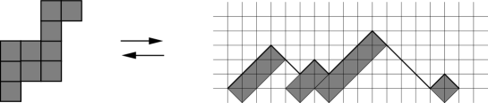
Figure 2: [88] A combinatorial bijection between staircase polygons and Dyck paths [21, 98]. Column heights of a polygon correspond to peak heights of a path.

For more about this connection, see the remark at the end of the following subsection.

3.4 $q$-difference equations

All polygon models discussed above have an algebraic perimeter generating function. Moreover, their half-perimeter and area generating function satisfies a functional equation of the form

$$P(x,q)=G(x,q,P(x,q),P(qx,q)),$$

for a real polynomial $G(x,q,y_{0},y_{1})$. Since, under mild assumptions on $G$, the equation reduces to an algebraic equation for $P(x,1)$ in the limit $q\to 1$, it may be viewed as a “deformation” of an algebraic equation. In this subsection, we will analyse equations of this type at the special point $(x,q)=(x_{c},1)$, where $x_{c}$ is the radius of convergence of $P(x,1)$. It will appear that the methods used in the above examples also can be applied to this more general case.

The above equation falls into the class of $q$-difference equations [103]. While particular examples appear in combinatorics in a number of places, see e.g. [37], the asymptotic behaviour of equations of the above form seems to have been systematically studied initially in [25, 87]. The study can be done in some generality, e.g., also for non-polynomial power series $G$, for replacements more general than $x\mapsto qx$, and for multivariate generalisations, see [89] and [25]. For simplicity, we will concentrate on polynomial $G$, and then briefly discuss generalisations. Our exposition closely follows [89, 87].

3.4.1 Algebraic $q$-difference equations

Definition 3 (Algebraic $q$-difference equation [25, 87]).

An algebraic $q$-difference equation is an equation of the form

$$P(x,q)=G(x,q,P(x,q),P(qx,q),\ldots,P(q^{N}x,q)),$$ (26)

where $G(x,q,y_{0},y_{1},\ldots,y_{N})$ is a complex polynomial. We require that

$$G(0,q,0,0,\ldots,0)\equiv 0,\qquad\frac{\partial G}{\partial y_{k}}(0,q,0,0,\ldots,0)\equiv 0\qquad(k=0,1,\ldots,N).$$

Remarks. i) See [103] for an overview of the theory of $q$-difference equations. As $q$ approaches unity, the above equation reduces to an algebraic equation.
ii) Asymptotics for solutions of algebraic $q$-difference equations have been considered in [25]. The above definition is a special case of [89, Def 2.4], where a multivariate extension is considered, and where $G$ may be non-polynomial. Also, replacements more general than $x\mapsto f(q)x$ are allowed. Such equations are called $q$-functional equations in [89]. The results presented below apply mutatis mutandis also to $q$-functional equations.

The algebraic $q$-difference equation in Definition 3 uniquely defines a (formal) power series $P(x,q)$ satisfying $P(0,q)\equiv 0$. This is shown by analysing the implied recurrence for the coefficients $p_{m}(q)$ of $P(x,q)=\sum_{m>0}p_{m}(q)x^{m}$, see also [89, Prop 2.5]. In fact, $p_{m}(q)$ is a polynomial in $q$. The growth of its degree in $m$ is not larger than $cm^{2}$ for some positive constant $c$, hence the counting parameters are rank 2 parameters [25]. In our situation, such a bound holds, since the area of a polygon grows at most quadratically with its perimeter.

From the preceding discussion, it follows that the factorial moment generating functions

$$g_{k}(x)=\frac{1}{k!}\left.\frac{\partial^{k}}{\partial q^{k}}P(x,q)\right|_{q=1}$$

are well-defined as formal power series. In fact, they can be recursively determined from the $q$-difference equation by implicit differentiation, as a consequence of the following proposition.

Proposition 5 ([87, 89]).

Consider the derivative of order $k>0$ of an algebraic $q$-difference equation Eq. (26) w.r.t. $q$, evaluated at $q=1$. It is linear in $g_{k}(x)$, and its r.h.s. is a complex polynomial in the power series $g_{l}(x)$ and its derivatives up to order $k-l$, where $l=0,\ldots,k$. ∎

Remarks. i) This statement can be shown by analysing the $k$-th derivative of the $q$-difference equation, using Faa di Bruno’s formula [18].
ii) It follows that every function $g_{k}(x)$ is rational in $g_{l}(x)$ and its derivatives up to order $k-l$, where $0\leq l<k$. Since $G$ is a polynomial, $g_{k}(x)$ is algebraic, by the closure properties of algebraic functions.

We discuss analytic properties of the (analytic continuations of the) factorial moment generating functions $g_{k}(x)$. These are determined by the analytic properties of $g_{0}(x)=P(x,1)$. We discuss the case of a square-root singularity of $P(x,1)$, which often occurs for combinatorial structures, and which is well studied, see e.g. [79, Thm 10.6] or [37, Ch VII.4]. Other cases may be treated similarly. We make the following assumption:

Assumption 2.

The $q$-difference equation in Definition 3 has the following properties:

• All coefficients of the polynomial $G(x,q,y_{0},y_{1},\ldots,y_{N})$ are non-negative.

• The polynomial $Q(x,y):=G(x,1,y,y,\ldots,y)$ satisfies $Q(x,0)\not\equiv 0$ and has degree at least two in $y$.

• $P(x,1)=\sum_{m\geq 1}p_{m}x^{m}$ is aperiodic, i.e., there exist indices $1\leq i<j<k$ such that $p_{i}p_{j}p_{k}\neq 0$, while $\gcd(j-i,k-i)=1$.

Remarks. i) The positivity assumption is natural for combinatorial constructions. There are, however, $q$-difference equations with negative coefficients, which arise from systems of $q$-difference equations with non-negative coefficients by reduction. Examples are convex polygons [87, Sec 5.4] and directed convex polygons, see below.
ii) Assumptions $i)$ and $ii)$ result in a square-root singularity as the dominant singularity of $P(x,1)$.
iii) Assumption $iii)$ implies that there is only one singularity of $P(x,1)$ on its circle of convergence. Since $P(x,1)$ has non-negative coefficients only, it occurs on the positive real half-line. The periodic case can be treated by a straightforward extension [37].

An application of the (complex) implicit function theorem ensures that $P(x,1)$ is analytic at the origin. It can be analytically continued, as long as the defining algebraic equation remains invertible. Together with the positivity assumption, one can conclude that there is a number $0<x_{c}<\infty$, such that the analytic continuation of $P(x,1)$ satisfies $y_{c}=\lim_{x\nearrow x_{c}}P(x,1)<\infty$, with

$$Q(x_{c},y_{c})=y_{c},\quad\left.\frac{\partial}{\partial y}Q(x_{c},y)\right|_{y=y_{c}}=1.$$

With the positivity assumption on the coefficients, it follows that

$$B:=\frac{1}{2}\left.\frac{\partial^{2}}{\partial y^{2}}Q(x_{c},y)\right|_{y=y_{c}}>0,\quad C:=\left.\frac{\partial}{\partial x}Q(x,y_{c})\right|_{x=x_{c}}>0.$$ (27)

These conditions characterise the singularity of $P(x,1)$ at $x=x_{c}$ as a square-root. It can be shown that there exists a locally convergent expansion of $P(x,1)$ about $x=x_{c}$, and that $P(x,1)$ is analytic for $|x|<x_{c}$. We have the following result. Recall that a function $f(z)$ is $\Delta$-regular if it is analytic in the indented disc $\Delta=\{z:|z|\leq x_{c}+\eta,|\operatorname{Arg}(z-x_{c})|\geq\phi\}$ for some $\eta>0$ and some $\phi$, where $0<\phi<\pi/2$.

Proposition 6 ([79, 37, 89]).

Given Assumption 2, the power series $P(x,1)$ is analytic at $x=0$, with radius of convergence $x_{c}$. Its analytic continuation is $\Delta$-regular, with a square-root singularity at $x=x_{c}$ and a local Puiseux expansion

$$P(x,1)=y_{c}+\sum_{l=0}^{\infty}f_{0,l}(1-x/x_{c})^{1/2+l/2},$$

where $y_{c}=\lim_{x\nearrow x_{c}}P(x,1)<\infty$ and $f_{0,0}=-\sqrt{x_{c}\,C/B}$, for constants $B>0$ and $C>0$ as in Eq. (27). The numbers $f_{0,l}$ can be recursively determined from the $q$-difference equation. ∎

The asymptotic behaviour of $P(x,1)=g_{0}(x)$ carries over to the factorial moment generating functions $g_{k}(x)$.

Proposition 7 ([89]).

Given Assumption 2, all factorial moment generating functions $g_{k}(x)$ are, for $k\geq 1$, analytic at $x=0$, with radius of convergence $x_{c}$. Their analytic continuations are $\Delta$-regular, with local Puiseux expansions

$$g_{k}(x)=\sum_{l=0}^{\infty}f_{k,l}(1-x/x_{c})^{-\gamma_{k}+l/2},$$

where $\gamma_{k}=3k/2-1/2$. The numbers $f_{k,0}=f_{k}$ are, for $k\geq 2$, characterised by the recursion

$$\gamma_{k-1}f_{k-1}+\frac{1}{4f_{1}}\sum_{l=0}^{k}f_{l}f_{k-l}=0,$$

and the numbers $f_{0}<0$ and $f_{1}>0$ are given by

$$f_{0}=-\sqrt{\frac{Cx_{c}}{B}},\qquad 4f_{1}=\frac{\sum_{k=1}^{N}k\frac{\partial G}{\partial y_{k}}(x_{c},1,y_{c},y_{c},\ldots,y_{c})}{B},$$ (28)

for constants $B>0$ and $C>0$ as in Eq. (27). ∎

Remarks. i) This result can be obtained by a direct analysis of the $q$-difference equation, applying Faa di Bruno’s formula, see also [87, Sec 2.2].
ii) Alternatively, it can be obtained by applying the method of dominant balance to the $q$-difference equation. To this end, one notes that all functions $g_{k}(x)$ are Laurent series in $\sqrt{1-x/x_{c}}$, and that their leading exponents are bounded from above by $\gamma_{k}$. (An upper bound on an exponent is usually easier to obtain than its exact value, since cancellations can be ignored). With these two ingredients, the method of dominant balance, as described above, can be applied. The differential equation of the function $F(s)$ then translates, via a transfer theorem, into the above recursion for the coefficients. See [89, Sec 5].

The above result can be used to infer the limit distribution of area, along the lines of Section 3.2.

Theorem 4 ([25, 89]).

Let Assumption 2 be satisfied. For the solution of an algebraic $q$-difference equation $P(x,q)=\sum_{m,n}p_{m,n}x^{m}q^{n}$, let $\widetilde{X}_{m}$ denote the random variable

$$\mathbb{P}(\widetilde{X}_{m}=n)=\frac{p_{m,n}}{\sum_{n}p_{m,n}}$$

(which is well-defined for almost all $m$). The mean of $\widetilde{X}_{m}$ is given by

$$\mathbb{E}[\widetilde{X}_{m}]\sim 2\sqrt{\pi}\frac{f_{1}}{|f_{0}|}m^{3/2}\qquad(m\to\infty),$$

where the numbers $f_{0}$ and $f_{1}$ are given in Eq. (28). The sequence of normalised random variables $X_{m}$ converges in distribution,

$$X_{m}=\frac{\widetilde{X}_{m}}{\mathbb{E}[\widetilde{X}_{m}]}\stackrel{{\scriptstyle d}}{{\longrightarrow}}\frac{Y}{\sqrt{\pi}}\qquad(m\to\infty),$$

where $Y$ is Airy distributed according to Definition 2. We also have moment convergence. ∎

Remarks. i) An explicit calculation shows that $\phi_{k}=|f_{0}|^{-1}\left(\frac{|f_{0}|}{2f_{1}}\right)^{k}f_{k}$. Together with Proposition 7, the claim of the proof follows by standard reasoning, as in the examples above.
ii) The above theorem appears in [25, Thm 3.1], together with an indication of the arguments of a proof. [There is a misprint in the definition of $\gamma$ in [25, Thm 3.1]. In our notation $\gamma=4Bf_{1}$.] Within the more general setup of $q$-functional equations, the theorem is a special case of [89, Thm 1.5].
iii) The above theorem is a kind of central limit theorem for combinatorial constructions, since the Airy distribution arises under natural assumptions for a large class of combinatorial constructions. For a connection to certain Brownian motion functionals, see below.

3.4.2 $q$-functional equations and other extensions

We discuss extensions of the above result. Generically, the dominant singularity of $P(x,1)$ is a square-root. The case of a simple pole as dominant singularity, which generalises the example of Ferrers diagrams, has been discussed in [87]. Under weak assumptions, the resulting limit distribution of area is concentrated. Other singularities can also be analysed, as shown in the examples of rectangles above and of directed convex polygons in the following subsection. Compare also [90].

The case of non-polynomial $G$ can be discussed along the same lines, with certain assumptions on the analyticity properties of the series $G$. In the undeformed case $q=1$, it is a classical result [37, Ch VII.3] that the generating function has a square-root as dominant singularity, as in the polynomial case. One can then argue along the above lines that an Airy distribution emerges as the limit law of the deformation variable [89, Thm 1.5]. Such an extension is relevant, since prominent combinatorial models, such as the Cayley tree generating function, fall into that class. See also the discussion of self-avoiding polygons below.

The above statements also remain valid for more general classes of replacements $x\mapsto qx$, e.g., for replacements $x\mapsto f(q)x$, where $f(q)$ is analytic for $0\leq q\leq 1$, with non-negative series coefficients about $q=0$. More interestingly, the idea of introducing a $q$-deformation may be iterated [25], leading to equations such as

$$P(x,q_{1},\ldots,q_{M})=G(x,P(xq_{1}\cdot\ldots\cdot q_{M},q_{1}q_{2}\cdot\ldots\cdot q_{M},q_{2}q_{3}\cdot\ldots\cdot q_{M},\ldots,q_{M})).$$ (29)

The counting parameters corresponding to $q_{k}$ are rank $k+1$ parameters, and limit distributions for such quantities have been derived for some types of singularities [77, 78, 88]. There is a central limit result for the generic case of a square-root singularity [89]. This generalisation applies to counting parameters, which decompose linearly under a combinatorial construction. These results can also be obtained by an alternative method, which generalises to non-linear parameters, see [51].

The case where the limit $q$ to unity in a $q$-difference equation is not algebraic, has not been discussed. For example, if $G(x,q,P(x,q),P(qx,q))=0$ for some polynomial $G$, the limit $q$ to unity might lead to an algebraic differential equation for $P(x,1)$. This may be seen by noting that

$$\lim_{q\to 1}\frac{f(x)-f(qx)}{(1-q)}=xf^{\prime}(x),$$

for $f(x)$ differentiable at $x$. Such equations are possibly related to polygon models such as three-choice polygons [44] or punctured staircase polygons [45]. Their perimeter generating function is not algebraic, hence the models do not satisfy an algebraic $q$-difference equation as in Definition 3.

3.4.3 A stochastic connection

Lastly, we indicate a link to Brownian motion, which appears in [99, 100] and was further developed in [77, 78, 89, 88]. As we saw in Section 3.2, limit distributions can, under certain conditions, be characterised by a certain Laplace transform of their moment generating functions. This approach, which arises naturally from the viewpoint of generating functions, can be applied to discrete versions of Brownian motion, excursions, bridges or meanders. Asymptotic results are results for the corresponding stochastic objects. In fact, distributions of some functionals of Brownian motion have apparently first been obtained using this approach [99, 100].

Interestingly, a similar characterisation appears in stochastics for functionals of Brownian motion, via the Feynman-Kac formula. For example, Louchard’s formula [66] relates the logarithmic derivate of the Airy function to a certain Laplace transform of the moment generating function of the law of the Brownian excursion area. Distributions of functionals of Brownian motion can also be obtained by a path integral approach, see [75] for a recent overview.

The discrete approach provides an alternative method for obtaining information about distributions of certain functionals of Brownian motion. For such functionals, it provides an alternative proof of Louchard’s formula [77, 78]. It leads, via the method of dominant balance, quite directly to moment recurrences for the underlying distribution. These have been studied in the case of rank $k$ parameters for discrete models of Brownian motion. In particular, they characterise the distributions of integrals over $(k-1)$-th powers of the corresponding stochastic objects [77, 78, 89, 88]. Such results have apparently not been previously derived using stochastic methods. The generating function approach can also be applied to classes of $q$-functional equations with singularities different from those connected to Brownian motion. For a related generalisation, see [10].

Vice versa, results and techniques from stochastics can be (and have been) analysed in order to study asymptotic properties of polygons. An example is the contour process of simply generated trees [38], which asymptotically describes the area of a staircase polygon. See also [69, 70, 71, 59].

3.5 Directed convex polygons

We show that the limit law of area of directed convex polygons in the uniform fixed perimeter ensemble is that of the area of the Brownian meander.

Fact 2 ([100, Thm 2]).

The random variable $Z$ of area of the Brownian meander is characterised by

$$\frac{\mathbb{E}[Z^{k}]}{k!}=\frac{\Gamma(\alpha_{0})}{\Gamma(\alpha_{k})}\frac{\omega_{k}}{\omega_{0}}\frac{1}{2^{k/2}},$$

where $\alpha_{k}=3k/2+1/2$. The numbers $\omega_{k}$ satisfy for $k\geq 1$ the quadratic recurrence

$$\alpha_{k-1}\omega_{k-1}+\sum_{l=0}^{k}\phi_{l}2^{-l}\omega_{k-l}=0,$$

with initial condition $\omega_{0}=1$, where the numbers $\phi_{k}$ appear in the Airy distribution as in Definition 2. ∎

Remarks. i) This result has been derived using a discrete meander, whose length and area generating function is described by a system of two algebraic $q$-difference equations, see [77, Prop 1].
ii) We have $\mathbb{E}[Z]=3\sqrt{2\pi}/8$ for the mean of $Z$. The random variable $Z$ is uniquely determined by its moments. The numbers $\omega_{k}$ appear in the asymptotic expansion [100, Thm 3]

$$\Omega(s)=\frac{1-3\int_{0}^{s}\operatorname{Ai}(t)\,{\rm d}t}{3\operatorname{Ai}(s)}\sim\sum_{k\geq 0}(-1)^{k}\omega_{k}s^{-\alpha_{k}}\qquad(s\to\infty),$$

where $\operatorname{Ai}(x)=\frac{1}{\pi}\int_{0}^{\infty}\cos(t^{3}/3+tx)\,{\rm d}t$ is the Airy function.

Explicit expressions have been derived for the moment generating function and for the distribution function of $Z$.

Fact 3 ([100, Thm 5]).

The moment generating function $M(t)=\mathbb{E}[\operatorname{e}^{-tZ}]$ of $Z$ satisfies the Laplace transform

$$\int_{0}^{\infty}\operatorname{e}^{-st}M(\sqrt{2}\,t^{3/2})\frac{1}{t^{1/2}}\,{\rm d}t=\sqrt{\pi}\,\Omega(s).$$ (30)

It is explicitly given by

$$M(t)=2^{-1/6}t^{1/3}\sum_{k=1}^{\infty}R_{k}\exp(-\beta_{k}t^{2/3}2^{-1/3})$$

for $\Re(t)>0$, where the numbers $-\beta_{k}$ are the zeroes of the Airy function, and where

$$R_{k}=\frac{\beta_{k}(1+3\int_{0}^{\beta_{k}}\operatorname{Ai}(-t)\,{\rm d}t)}{3\operatorname{Ai}^{\prime}(-\beta_{k})}.$$

The random variable $Z$ has a continuous density $p(y)$, with distribution function $R(x)=\int_{0}^{x}p(y)\,{\rm d}y$ given by

$$R(x)=\frac{\sqrt{\pi}}{(18)^{1/6}x}\sum_{k=1}^{\infty}R_{k}\operatorname{e}^{-v_{k}}v_{k}^{-1/3}\operatorname{Ai}((3v_{k}/2)^{2/3}),$$

where $v_{k}=(\beta_{k})^{3}/(27x^{2})$.∎

Remark. The moment generating function and the distribution function are obtained by two consecutive inverse Laplace transforms of Eq. (30).

Theorem 5.

The normalised area random variables $X_{m}$ of directed convex polygons Eq. (18) satisfy

$$X_{m}\stackrel{{\scriptstyle d}}{{\longrightarrow}}\frac{1}{2}Z\qquad(m\to\infty),$$

where $Z$ is the area random variable of the Brownian meander as in Fact 2. We also have moment convergence.

Proof.

A system of $q$-difference equations for the generating function $Q(x,y,q)$ of directed convex polygons, counted by width, height and area, has been given in [9, Lemma 1.1]. It can be reduced to a single equation,

$$\begin{split}&q(qx-1)Q(x,y,q)+\left((1+q)(P(x,y,q)+y)\right)Q(qx,y,q)+\\ &\left(xyq-y^{2}+P(x,y,q)(qx-y-1)\right)Q(q^{2}x,y,q)\\ &-q^{2}xy\left(y+P(x,y,q)-1\right)=0,\end{split}$$ (31)

where $P(x,y,q)$ is the width, height and area generating function of staircase polygons. Setting $q$=1 and $x=y$ yields the half-perimeter generating function

$$g_{0}(x)=\frac{x^{2}}{\sqrt{1-4x}}.$$

Hence $x_{c}=1/4$ for the radius of convergence of $Q(x,x,1)$.

It is possible to derive from Eq. (31) a $q$-difference equation for the (isotropic) half-perimeter and area generating function $Q(x,q)=Q(x,x,q)$ of directed convex polygons. This is due to the symmetry $Q(x,y,q)=Q(y,x,q)$, which results from invariance of the set of directed convex polygons under reflection along the negative diagonal $y=-x$. Since this equation is quite long, we do not give it here. By arguments analogous to those of the previous subsection, it can be deduced from this equation that all area moment generating functions $g_{k}(x)$ of $Q(x,1)$ are Laurent series in $s=\sqrt{1-4x}$, see also [89, Prop (4.3)]. The leading singular exponent of $g_{k}(x)$, defined by $g_{k}(x)\sim h_{k}(1-x/x_{c})^{-\alpha_{k}}$ as $x\nearrow x_{c}$, can be bounded from above by $\alpha_{k}\leq 3k/2+1/2$, see also [89, Prop (4.4)] for the argument. We apply the method of dominant balance, in order to prove that $\alpha_{k}=3k/2+1/2$ and to yield recurrences for the coefficients $h_{k}$. We define

$$\begin{split}P(x,q)&=\frac{1}{4}+(1-q)^{1/3}F\left(\frac{1-4x}{(1-q)^{2/3}},(1-q)^{1/3}\right),\\ Q(x,q)&=(1-q)^{-1/3}H\left(\frac{1-4x}{(1-q)^{2/3}},(1-q)^{1/3}\right),\end{split}$$

where $F(s)=F(s,0)$ has already been determined in Eq. (25). We set $4x=1-s\epsilon^{2}$, $q=1-\epsilon^{3}$, and expand the $q$-difference equation to leading order in $\epsilon$. We get for $H(s):=H(s,0)$ the inhomogeneous linear differential equation of first order

$$H^{\prime}(s)+4H(s)F(s)+\frac{1}{8}=0.$$

This implies for the coefficients $h_{k}$ of $H(s)=\sum_{k\geq 0}h_{k}s^{-\alpha_{k}}$ and $f_{k}$ of $F(s)=\sum_{k\geq 0}f_{k}s^{-\gamma_{k}}$ for $k\geq 1$ the quadratic recursion

$$\alpha_{k-1}h_{k-1}+4\sum_{l=0}^{k}f_{l}h_{k-l}=0,$$

where $h_{0}=1/16$. Using $f_{k}=2^{-2k-1}\phi_{k}$, we obtain the meander recursion in Fact 2 by setting $h_{k}=2^{-k-4}\omega_{k}$. It can be inferred from the functional equation that (the analytic continuations of) all factorial moment generating functions are $\Delta$-regular, with $x_{c}=1/4$. Thus Lemma 2 applies, and we conclude $X_{m}\stackrel{{\scriptstyle d}}{{\to}}Z/2$. ∎∎

Remarks. i) The above theorem states that the limit distribution of area of directed convex polygons coincides, up to normalisation, with the area distribution of the Brownian meander [100]. This suggests that there might exist a combinatorial bijection to discrete meanders, in analogy to that between staircase polygons and Dyck paths. Up to now, a “nice” bijection has not been found, see however [6, 72] for combinatorial bijections to discrete bridges.
ii) The above proof relies on a $q$-difference equation for the isotropic generating function $Q(x,x,q)$. Up to normalisation, the meander distribution also appears for the anisotropic model $Q(x,y,q)$, where $0<y<1/2$ is fixed, as can be shown by a considerably simpler calculation. The normalisation constant coincides with that of the isotropic model for $y=1/2$. The latter statement is also a consequence of the fact that the height random variable of directed polygons is asymptotically Gaussian, after centering and normalisation. Analogous considerations apply to the relation between isotropic and anisotropic versions of the other polygon classes.

3.6 Limit laws away from $(x_{c},1)$

As motivated in the introduction, limit laws in the fixed perimeter ensemble for $q\neq 1$ are expected to be Gaussian. The same remark holds for the fixed area ensemble for $x\neq x_{c}$. There are partial results for the model of staircase polygons. The fixed area ensemble can, for $x<x_{c}$ and $q$ near unity, be analysed using Fact 7 of the following section. For staircase polygons in the uniform fixed area ensemble $x=1$, the following result holds.

Fact 4 ([37, Prop IX.11]).

Consider the perimeter random variable of staircase polygons in the uniform fixed area ensemble,

$$\mathbb{P}(\widetilde{Y}_{n}=m)=\frac{p_{m,n}}{\sum_{m}p_{m,n}}.$$

The variable $\widetilde{Y}_{n}$ has mean $\mu_{n}\sim\mu\cdot n$ and standard deviation $\sigma_{n}\sim\sigma\sqrt{n}$, where the numbers $\mu$ and $\sigma$ satisfy

$$\mu=0.8417620156\ldots,\qquad\sigma=0.4242065326\ldots$$

The centred and normalised random variables

$$Y_{n}=\frac{\widetilde{Y}_{n}-\mu_{n}}{\sigma_{n}},$$

converge in distribution to a Gaussian random variable. ∎

Remark. The above result is proved using an explicit expression for the half-perimeter and area generating function, as a ratio of two $q$-Bessel functions. It can be shown that this expression is meromorphic about $(x,q)=(1,q_{c})$ with a simple pole, where $q_{c}$ is the radius of convergence of the generating function $P(1,q)$. The explicit form of the singularity about $(1,q_{c})$ yields a Gaussian limit law.

There are a number of results for classes of column-convex polygons in the uniform fixed area ensemble, typically leading to Gaussian limit laws. The upper and lower shape of a polygon can be described by Brownian motions. See [69, 70, 71] for details. It would be interesting to prove convergence to a Gaussian limit law within a more general framework, such as $q$-difference equations. Analogous questions for other functional equations, describing counting parameters such as horizontal width, have been studied in [24].

3.7 Self-avoiding polygons

A numerical analysis of self-avoiding polygons, using data from exact enumeration [91, 92], supports the conjecture that the limit law of area is, up to normalisation, the Airy distribution.

Let $p_{m,n}$ denote the number of square lattice self-avoiding polygons of half-perimeter $m$ and area $n$. Exact enumeration techniques have been applied to obtain the numbers $p_{m,n}$ for all values of $n$ for given $m\leq 50$. Numerical extrapolation techniques yield very accurate estimates of the asymptotic behaviour of the coefficients of the factorial moment generating functions. To leading order, these are given by

$$[x^{m}]g_{k}(x)=\frac{1}{k!}\sum_{n}(n)_{k}p_{m,n}\sim A_{k}x_{c}^{-m}m^{3k/2-3/2-1}\qquad(m\to\infty),$$ (32)

for positive amplitudes $A_{k}$. The above form has been numerically checked [91, 92] for values $k\leq 10$ and is conjectured to hold for arbitrary $k$. The value $x_{c}$ is the radius of convergence of the half-perimeter generating function of self-avoiding polygons. The amplitudes $A_{k}$ have been extrapolated to at least five significant digits. In particular, we have

$$x_{c}=0.14368062927(2),\qquad A_{0}=0.09940174(4),\qquad A_{1}=0.0397886(1),$$

where the numbers in brackets denote the uncertainty in the last digit. An exact value of the amplitude $A_{1}=1/(8\pi)$ has been predicted [15] using field-theoretic arguments.

The particular form of the exponent implies that the model of rooted self-avoiding polygons $\widetilde{p}_{m,n}=mp_{m,n}$ has the same exponents $\phi=2/3$ and $\theta=1/3$ as staircase polygons. In particular, it implies a square-root as dominant singularity of the half-perimeter generating function. Together with the above result for $q$-functional equations, this suggests that (rooted) self-avoiding polygons might obey the Airy distribution as a limit law of area.

A natural method to test this conjecture consists in analysing ratios of moments, such that a normalisation constant is eliminated. Such ratios are also called universal amplitude ratios. If the conjecture were true, we would have asymptotically

$$\frac{\mathbb{E}[\widetilde{X}_{m}^{k}]}{\mathbb{E}[\widetilde{X}_{m}]^{k}}\sim k!\frac{\Gamma(\gamma_{1})^{k}}{\Gamma(\gamma_{k})\Gamma(\gamma_{0})^{k-1}}\frac{\phi_{k}\phi_{0}^{k-1}}{\phi_{1}^{k}}\qquad(m\to\infty),$$

for the area random variables $\widetilde{X}_{m}$ as in Eq. (17). The numbers $\phi_{k}$ and exponents $\gamma_{k}$ are those of the Airy distribution as in Definition 2. The above form was numerically confirmed for values of $k\leq 10$ to a high level of numerical accuracy. The normalisation constant is obtained by noting that $\mathbb{E}[Y]=\sqrt{\pi}$.

Conjecture 1 (cf [91, 92]).

Let $p_{m,n}$ denote the number of square lattice self-avoiding polygons of half-perimeter $m$ and area $n$. Let $\widetilde{X}_{m}$ denote the random variable of area in the uniform fixed perimeter ensemble,

$$\mathbb{P}(\widetilde{X}_{m}=n)=\frac{p_{m,n}}{\sum_{n}p_{m,n}}.$$

We conjecture that

$$\frac{\widetilde{X}_{m}}{\mathbb{E}[\widetilde{X}_{m}]}\stackrel{{\scriptstyle d}}{{\longrightarrow}}\frac{Y}{\sqrt{\pi}},$$

where $Y$ is Airy distributed according to Definition 2.

Remarks. i) Field theoretic arguments [15] yield $A_{1}=1/(8\pi)$.
ii) References [91, 92] contain conjectures for the scaling function of self-avoiding polygons and rooted self-avoiding polygons, see the following section. In fact, the numerical analysis in [91, 92] mainly concerns the area amplitudes $A_{k}$, which determine the limit distribution of area.
iii) The area law of self-avoiding polygons has also been studied [91, 92] on the triangular and hexagonal lattices. As for the square lattice, the area limit law appears to be the Airy distribution, up to normalisation.
iv) It is an open question whether there are non-trivial counting parameters other than the area, whose limit law (in the fixed perimeter ensembles) coincides between self-avoiding polygons and staircase polygons. See [88] for a negative example. This indicates that underlying stochastic processes must be quite different.
v) A proof of the above conjecture is an outstanding open problem. It would be interesting to analyse the emergence of the Airy distribution using stochastic Loewner evolution [60]. Self-avoiding polygons at criticality are conjectured to describe the hull of critical percolation clusters and the outer boundary of two-dimensional Brownian motion [60].

A numerical analysis of the fixed area ensemble along the above lines again shows behaviour similar to that of staircase polygons. This supports the following conjecture.

Conjecture 2.

Consider the perimeter random variable of self-avoiding polygons in the uniform fixed area ensemble,

$$\mathbb{P}(\widetilde{Y}_{n}=m)=\frac{p_{m,n}}{\sum_{m}p_{m,n}}.$$

The random variable $\widetilde{Y}_{n}$ is conjectured to have mean $\mu_{n}\sim\mu\cdot n$ and standard deviation $\sigma_{n}\sim\sigma\sqrt{n}$, where the numbers $\mu$ and $\sigma$ satisfy

$$\mu=1.855217(1),\qquad\sigma^{2}=0.3259(1),$$

where the number in brackets denotes the uncertainty in the last digit. The centred and normalised random variables

$$Y_{n}=\frac{\widetilde{Y}_{n}-\mu_{n}}{\sigma_{n}},$$

are conjectured to converge in distribution to a Gaussian random variable.

The above conjectures, together with the results of the previous subsection, also raise the question whether rooted square-lattice self-avoiding polygons, counted by half-perimeter and area, might satisfy a $q$-functional equation. In particular, it would be interesting to consider whether rooted self-avoiding polygons might satisfy

$$P(x)=G(x,P(x)),$$ (33)

for some power series $G(x,y)$ in $x,y$. If the perimeter generating function $P(x)$ is not algebraic, this excludes polynomials $G(x,y)$ in $x$ and $y$. Note that the anisotropic perimeter generating function of self-avoiding polygons is not $D$-finite [86]. It is thus unlikely that the isotropic perimeter generating function is $D$-finite and, in particular, algebraic. On the other hand, solutions of Eq. (33) need not be algebraic nor $D$-finite. An example is the Cayley tree generating function $T(x)$ satisfying $T(x)=x\exp(T(x))$, see [33].

3.8 Punctured polygons

Punctured polygons are self-avoiding polygons with internal holes, which are also self-avoiding polygons. The polygons are also mutually avoiding. The perimeter of a punctured polygon is the sum of the lengths of its boundary curves, the area of a punctured polygon is the area of the outer polygon minus the area of the holes. Apart from intrinsic combinatorial interest, models of punctured polygons may be viewed as arising from two-dimensional sections of three-dimensional self-avoiding vesicles. Counted by area, they may serve as an approximation to the polyomino model.

We consider, for a given subclass of self-avoiding polygons, punctured polygons with holes from the same subclass. The case of a bounded number of punctures of bounded size can be analysed in some generality. The case of a bounded number of punctures of unbounded size leads to simple results if the critical perimeter generating function of the model without punctures is finite.

For a given subclass of self-avoiding polygons, the number $p_{m,n}$ denotes the number of polygons with half-perimeter $m$ and area $n$. Let $p_{m,n}^{(r,s)}$ denote the number of polygons with $r\geq 1$ punctures whose half-perimeter sum equals $s$. Let $p_{m,n}^{(r)}$ denote the number of polygons with $r\geq 1$ punctures of arbitrary size.

Theorem 6 ([94, Thms 1,2]).

Assume that, for a class of self-avoiding polygons without punctures, the area moment coefficients $p_{m}^{(k)}=\sum_{n\geq 0}n^{k}p_{m,n}$ have, for $k\in\mathbb{N}_{0}$, the asymptotic form

$$p_{m}^{(k)}\sim A_{k}x_{c}^{-m}m^{\gamma_{k}-1}\qquad(m\to\infty),$$

for numbers $A_{k}>0$, for $0<x_{c}\leq 1$ and for $\gamma_{k}=(k-\theta)/\phi$, where $0<\phi<1$. Let $g_{0}(x)=\sum_{m\geq 0}p_{m}^{(0)}x^{m}$ denote the half-perimeter generating function.

Then, the area moment coefficient $p_{m}^{(r,k,s)}=\sum_{n}n^{k}p_{m,n}^{(r,s)}$ of the polygon class with $r\geq 1$ punctures whose half-perimeter sum equals $s$ is, for $k\in\mathbb{N}_{0}$, asymptotically given by

$$p_{m}^{(r,k,s)}\sim A_{k}^{(r,s)}x_{c}^{-m}m^{\gamma_{k+r}-1}\qquad(m\to\infty),$$

where $A_{k}^{(r,s)}=\frac{A_{k+r}}{r!}x_{c}^{s}[x^{s}](g_{0}(x))^{r}$.

If $\theta>0$, the area moment coefficient $p_{m}^{(r,k)}=\sum_{n}n^{k}p_{m,n}^{(r)}$ of the polygon class with $r\geq 1$ punctures of arbitrary size satisfies, for $k\in\mathbb{N}_{0}$, asymptotically

$$p_{m}^{(r,k)}\sim A_{k}^{(r)}x_{c}^{-m}m^{\gamma_{k+r}-1}\qquad(m\to\infty),$$

where the amplitudes $A_{k}^{(r)}$ are given by

$$A_{k}^{(r)}=\frac{A_{k+r}(g_{0}(x_{c}))^{r}}{r!}.$$

∎

Remarks. i) The basic argument in the proof of the preceding result involves an estimate of interactions of hole polygons with one another or with the boundary of the external polygon, which are shown to be asymptotically irrelevant. This argument also applies in higher dimensions, as long as the exponent $\phi$ satisfies $0<\phi<1$.
ii) In the case of an infinite critical perimeter generating function, such as for subclasses of convex polygons, boundary effects are asymptotically relevant, if punctures of unbounded size are considered. The case of an unbounded number of punctures, which approximates the polyomino problem, is unsolved.
iii) The above result leads to new area limit distributions. For rectangles with $r$ punctures of bounded size, we get $\beta_{r+1,1/2}$ as the limit distribution of area. For staircase polygons with punctures, we obtain generalisations of the Airy distribution, which are discussed in [94]. In contrast, for Ferrers diagrams with punctures of bounded size, the limit distribution of area stays concentrated.
iv) The theorem also applies to models of punctured polygons, which do not satisfy an algebraic $q$-difference equation. An example is given by staircase polygons with a staircase hole of unbounded size, whose perimeter generating function is not algebraic [45].

3.9 Models in three dimensions

There are very few results for models in higher dimensions, notably for models on the cubic lattice. There are a number of natural counting parameters for such objects. We restrict consideration to area and volume, which is the three-dimensional analogue of perimeter and area of two-dimensional models.

One prominent model is self-avoiding surfaces on the cubic lattice, also studied as a model of three-dimensional vesicle collapse. We follow the review in [102] (see also the references therein) and consider closed orientable surfaces of genus zero, i.e., surfaces homeomorphic to a sphere. Numerical studies indicate that the surface generating function displays a square-root $\gamma=-1/2$ as the dominant singularity.

Consider the fixed surface area ensemble with weights proportional to $q^{n}$, with $n$ the volume of the surface. One expects a deflated phase (branched polymer phase) for small values of $q$ and an inflated phase (spherical phase) for large values of $q$. In the deflated phase, the mean volume of a surface should grow proportionally to the area $m$ of the surface, in the inflated phase the mean volume should grow like $m^{3/2}$ with the surface. Numerical simulations suggest a phase transition at $q=1$ with exponent $\phi=1$. This indicates that a typical surface resembles a branched polymer, and a concentrated distribution of volume is expected. Note that this behaviour differs from that of the two-dimensional model of self-avoiding polygons.

Even relatively simple subclasses of self-avoiding surfaces such as rectangular boxes [73] and plane partition vesicles [50], generalising the two-dimensional models of rectangles and Ferrers diagrams, display complicated behaviour. Let $p_{m,n}$ denote the number of surfaces of area $m$ and volume $n$ and consider the generating function $P(x,q)=\sum_{m,n}p_{m,n}x^{m}q^{n}$. For rectangular box vesicles, we apparently have $P(x,1)\sim A|\log(1-x)|/(1-x)^{3/2}$ as $x\to 1^{-}$, some some constant $A>0$, see [73, Eq (35)]. In the fixed surface area ensemble, a linear polymer phase $0<q<1$ is separated from a cubic phase $q>1$. At $q=1$, we have $\phi=2/3$, such that typical rectangular boxes are expected to attain a cubic shape. We expect a limit distribution which is concentrated. For plane partition vesicles, it is conjectured on the basis of numerical simulations [50, Sec 4.1.1] that $P(x,1)\sim A\exp(\alpha/(x_{c}-x)^{1/3})/(x_{c}-x)^{\gamma}$, where $\gamma\approx 1.7$ at $x_{c}=0.8467(3)$, for non-vanishing constants $A$ and $\alpha$. It is expected that $\phi=1/2$.

As in the previous subsection, three-dimensional models of punctured vesicles may be considered. The above arguments hold, if the exponent $\phi$ satisfies $0<\phi<1$. A corresponding result for punctures of unbounded size can be stated if the critical surface area generating function is finite.

3.10 Summary

In this section, we described methods to extract asymptotic area laws for polygon models on the square lattice, and we applied these to various classes of polygons. Some of the laws were found to coincide with those of the (absolute) area under a Brownian excursion and a Brownian meander. A combinatorial explanation for the latter result has not been given. Is there a simple polygon model with the same area limit law as the area under a Brownian bridge? The connection to stochastics deserves further investigation. In particular, it would be interesting to identify underlying stochastic processes. For an approach to a number of different random combinatorial structures starting from a probabilistic viewpoint, see [82].

Area laws of polygon models in the uniform fixed perimeter ensemble $q=1$ have been understood in some generality, by an analysis of the singular behaviour of $q$-functional equations about the point $(x,q)=(x_{c},1)$. Essentially, the type of singularity of the half-perimeter generating function determines the limit law. A refined analysis can be done, leading to local limit laws and providing convergence rates. Also, limit distributions describing corrections to the asymptotic behaviour can be derived. They seem to coincide with distributions arising in models of punctured polygons, see [94].

For non-uniform ensembles, concentrated distributions are expected, but general results, e.g. for $q$-functional equations, are lacking. These may be obtained by multivariate singularity analysis, see also [24, 65].

The underlying structure of $q$-functional equations appears in a number of other combinatorial models, such as models of two-dimensional directed walks, counted by length and area between the walk and the $x$-axis, models of simply generated trees, counted by the number of nodes and path length, and models which appear in the average case analysis of algorithms, see [34, 37]. Thus, the above methods and results can be applied to such models. In statistical physics, this mainly concerns models of (interacting) directed walks, see [48] for a review. There is also an approach to the behaviour of such walks from a stochastic viewpoint, see e.g. the review [101].

There are exactly solvable polygon models, which do not satisfy an algebraic $q$-difference equation, such as three-choice polygons [44], punctured staircase polygons [45], prudent polygon subclasses [96], and possibly diagonally convex polygons. For a rigorous analysis of the above models, it may be necessary to understand $q$-difference equations with more general holonomic solutions, as $q$ approaches unity.

Focussing on self-avoiding polygons, it might be interesting to analyse whether the perimeter generating function of rooted self-avoiding polygons might satisfy an implicit equation Eq. (33). Asymptotic properties of the area can possibly be studied using stochastic Loewner evolution [60]. Another open question concerns the area limit law for $q\neq 1$ or the perimeter limit law for $x\neq x_{c}$, where Gaussian behaviour is expected. At present, even the simpler question of analyticity of the critical curve $x_{c}(q)$ for $0<q<1$ is open.

Most results of this section concerned area limit laws of polygon models. Similarly, one can ask for perimeter laws in the fixed area ensemble. Results have been given for the uniform ensemble. Generally, Gaussian limit laws are expected away from criticality, i.e., away from $x=x_{c}$. Perimeter laws are more difficult to extract from a $q$-functional equation than area laws. We will however see in the following section that, surprisingly, under certain conditions, knowledge of the area limit law can be used to infer the perimeter limit law at criticality.

4 Scaling functions

From a technical perspective, the focus in the previous section was on the singular behaviour of the single-variable factorial moment generating function $g_{k}(x)$ Eq. (1), and on the associated asymptotic behaviour of their coefficients. This yielded the limiting area distribution of some polygon models.

In this section, we discuss the more general problem of the singular behaviour of the two-variable perimeter and area generating function of a polygon model. Near the special point $(x,q)=(x_{c},1)$, the perimeter and area generating function $P(x,q)=\sum_{m\geq 0}p_{m}(q)x^{m}=\sum_{n\geq 0}a_{n}(x)q^{n}$ is expected to be approximated by a scaling function, and the corresponding coefficient functions $p_{m}(q)$ and $a_{n}(x)$ are expected to be approximated by finite size scaling functions. As we will see, scaling functions encapsulate information about the limit distributions discussed in the previous section, and thus have a probabilistic interpretation.

We will give a focussed review, guided by exactly solvable examples, since singularity analysis of multivariate generating functions is, in contrast to the one-variable case, not very well developed, see [81] for a recent overview. Methods of particular interest to polygon models concern asymptotic expansions about multicritical points, which are discussed for special examples in [80, 5]. Conjectures for the behaviour of polygon models about multicritical points arise from the physical theory of tricritical scaling [41], see the review [61], which has been adapted to polygon models [14, 13]. There are few rigorous results about scaling behaviour of polygon models, which we will discuss. This will complement the exposition in [47]. See also [42, Ch 9] for the related subject of scaling in percolation.

4.1 Scaling and finite size scaling

The half-perimeter and area generating function of a polygon model $P(x,q)$ about $(x,q)=(x_{c},1)$ is expected to be approximated by a scaling function. This is motivated by the following heuristic argument. Assume that the factorial area moment generating functions $g_{k}(x)$ Eq. (1) have, for values $x<x_{c}$, a local expansion about $x=x_{c}$ of the form

$$g_{k}(x)=\sum_{l\geq 0}\frac{f_{k,l}}{(1-x/x_{c})^{\gamma_{k,l}}},$$

where $\gamma_{k,l}=(k-\theta_{l})/\phi$ and $\theta_{l+1}>\theta_{l}$. Disregarding questions of analyticity, we argue

$$\begin{split}P(x,q)&\approx\sum_{k\geq 0}(-1)^{k}\left(\sum_{l\geq 0}\frac{f_{k,l}}{(1-x/x_{c})^{\gamma_{k,l}}}\right)(1-q)^{k}\\ &\approx\sum_{l\geq 0}(1-q)^{\theta_{l}}\left(\sum_{k\geq 0}(-1)^{k}f_{k,l}\left(\frac{1-x/x_{c}}{(1-q)^{\phi}}\right)^{-\gamma_{k,l}}\right).\end{split}$$

In the above calculation, we replaced $P(x,q)$ by its Taylor series about $q=1$, and then replaced the Taylor coefficients by their expansion about $x=x_{c}$. The preceding heuristic calculation has, for some polygon models and on a formal level, a rigorous counterpart, see the previous section. In the above expression, the r.h.s. depends on series ${\cal F}_{l}(s)=\sum_{k\geq 0}(-1)^{k}f_{k,l}s^{-\gamma_{k,l}}$ of a single variable of combined argument $s=(1-x/x_{c})/(1-q)^{\phi}$. Restricting to the leading term $l=0$, this motivates the following definition. For $\phi>0$ and $x_{c}>0$, we define for numbers $s_{-},s_{+}\in[-\infty,+\infty]$ the domain

$$D(s_{-},s_{+})=\{(x,q)\in(0,\infty)\times(0,1):s_{-}<(1-x/x_{c})/(1-q)^{\phi}<s_{+})\}.$$

Definition 4 (Scaling function).

For numbers $p_{m,n}$ with generating function $P(x,q)=\sum_{m,n}p_{m,n}x^{m}q^{n}$, let Assumption 1 be satisfied. Let $0<x_{c}\leq 1$ be the radius of convergence of $P(x,1)$. Assume that there exist constants $s_{-},s_{+}\in[-\infty,+\infty]$ satisfying $s_{-}<s_{+}$ and a function ${\cal F}:(s_{-},s_{+})\to\mathbb{R}$, such that $P(x,q)$ satisfies, for real constants $\theta$ and $\phi>0$,

$$P^{(sing)}(x,q)\sim(1-q)^{\theta}{\cal F}\left(\frac{1-x/x_{c}}{(1-q)^{\phi}}\right)\qquad(x,q)\to(x_{c},1)\mbox{ in }D(s_{-},s_{+}).$$ (34)

Then, the function ${\cal F}(s)$ is called an (area) scaling function, and $\theta$ and $\phi$ are called critical exponents.

Remarks. i) In analogy to the one-variable case, the above asymptotic equality means that there exists a power series $P^{(reg)}(x,q)$ convergent for $|x|<x_{1}$ and $|q|<q_{1}$, where $x_{1}>x_{c}$ and $q_{1}>1$, such that the function $P^{(sing)}(x,q):=P(x,q)-P^{(reg)}(x,q)$ is asymptotically equal to the r.h.s..
ii) Due to the region $D(s_{-},s_{+})$ where the limit $(x,q)\to(x_{c},1)$ is taken, admissible values $(x,q)$ satisfy $0<q<1$ and $0<x<x_{0}(q)$, where $x_{0}(q)=x_{c}(1-s_{-}(1-q)^{\phi})$, if $s_{-}\neq-\infty$. Thus, in this case, the critical curve $x_{c}(q)$ satisfies $x_{c}(q)\geq x_{0}(q)$ as $q$ approaches unity. Note that equality need not hold in general.
iii) The method of dominant balance was originally applied in order to obtain a defining equation for a scaling function ${\cal F}(s)$ from a given functional equation of a polygon model. This assumes the existence of a scaling function, together with additional analyticity properties. See [84, 91, 87].
iv) For particular examples, an analytic scaling function ${\cal F}(s)$ exists, with an asymptotic expansion about infinity, and the area amplitude series $F(s)$ agrees with the asymptotic series, see below.
v) There is an alternative definition of a scaling function [31] by demanding

$$P^{(sing)}(x,q)\sim\frac{1}{(1-x/x_{c})^{-\theta/\phi}}{\cal H}\left(\frac{1-q}{(1-x/x_{c})^{1/\phi}}\right)\qquad(x,q)\to(x_{c},1)$$ (35)

in a suited domain, for a function ${\cal H}(t)$ of argument $t=(1-q)/(1-x/x_{c})^{1/\phi}$. Such a scaling form is also motivated by the above argument. One may then call such a function ${\cal H}(t)$ a perimeter scaling function. If ${\cal F}(s)$ is a scaling function, then a function ${\cal H}(t)$, satisfying Eq. (35) in a suited domain, is given by

$${\cal H}(t)=t^{\theta}{\cal F}(t^{-\phi}).$$

If $s_{-}\leq 0$ and $s_{+}=\infty$, the particular scaling form Eq. (34) implies a certain asymptotic behaviour of the critical area generating function and of the half-perimeter generating function. The following lemma is a consequence of Definition 4.

Lemma 3.

Let the assumptions of Definition 4 be satisfied.

• If $s_{+}=\infty$ and if the scaling function ${\cal F}(s)$ has the asymptotic behaviour

  $${\cal F}(s)\sim f_{0}s^{-\gamma_{0}}\qquad(s\to\infty),$$

  then $\gamma_{0}=-\frac{\theta}{\phi}$, and the half-perimeter generating function $P(x,1)$ satisfies

  $$P^{(sing)}(x,1)\sim f_{0}(1-x/x_{c})^{\theta/\phi}\qquad(x\nearrow x_{c}).$$

• If $s_{-}\leq 0$ and if the scaling function $\mathcal{F}(s)$ has the asymptotic behaviour

  $${\cal F}(s)\sim h_{0}s^{\alpha_{0}}\qquad(s\searrow 0),$$

  then $\alpha_{0}=0$, and the critical area generating function $P(x_{c},q)$ satisfies

  $$P^{(sing)}(x_{c},q)\sim h_{0}(1-q)^{\theta}\qquad(q\nearrow 1).$$

∎

A sufficient condition for equality of the area amplitude series and the scaling function is stated in the following lemma, which is an extension of Lemma 3.

Lemma 4.

Let the assumptions of Definition 4 be satisfied.

• Assume that the relation Eq. (34) remains valid under arbitrary differentiation w.r.t. $q$. If $s_{+}=\infty$, if the scaling function ${\cal F}(s)$ has an asymptotic expansion

  $${\cal F}(s)\sim\sum_{k\geq 0}(-1)^{k}f_{k}s^{-\gamma_{k}}\qquad(s\to\infty),$$

  and if an according asymptotic expansion is true for arbitrary derivatives, then the following statements hold.

  • The exponent $\gamma_{k}$ is, for $k\in\mathbb{N}_{0}$, given by

    $$\gamma_{k}=\frac{k-\theta}{\phi}.$$

  • The scaling function ${\cal F}(s)$ determines the asymptotic behaviour of the factorial area moment generating functions via

    $$\left(\frac{1}{k!}\left.\frac{\partial^{k}}{\partial q^{k}}P(x,q)\right|_{q=1}\right)^{(sing)}\sim\frac{f_{k}}{(1-x/x_{c})^{\gamma_{k}}}\qquad(x\nearrow x_{c}).$$

• Assume that the relation Eq. (34) remains valid under arbitrary differentiation w.r. to $x$. If $s_{-}\leq 0$, and if the scaling function $\mathcal{F}(s)$ has an asymptotic expansion

  $$\mathcal{F}(s)\sim\sum_{k\geq 0}(-1)^{k}h_{k}s^{\alpha_{k}}\qquad(s\searrow 0),$$

  and if an according asymptotic expansion is true for arbitrary derivatives, then the following statements hold.

  • The exponent $\alpha_{k}$ is, for $k\in\mathbb{N}_{0}$, given by $\alpha_{k}=k$.

  • The scaling function determines the asymptotic behaviour of the factorial perimeter moment generating functions at $x=x_{c}$ via

    $$\begin{split}\left(\frac{1}{k!}\left.\frac{\partial^{k}}{\partial x^{k}}P(x,q)\right|_{x=x_{c}}\right)^{(sing)}\sim\frac{x_{c}^{-k}h_{k}}{(1-q)^{\beta_{k}}}\qquad(q\nearrow 1),\\ \end{split}$$

    where $\beta_{k}=k\phi-\theta$.

∎

Remarks. Lemma 4 states conditions under which the area amplitude series coincides with the scaling function. Given these conditions, the scaling function also determines the perimeter law of the polygon model at criticality.

In the one-variable case, the singular behaviour of a generating function translates, under suitable assumptions, to the asymptotic behaviour of its coefficients. We sketch the analogous situation for the asymptotic behaviour of a generating function involving a scaling function.

Definition 5 (Finite size scaling function).

For numbers $p_{m,n}$ with generating function $P(x,q)=\sum_{m,n}p_{m,n}x^{m}q^{n}$, let Assumption 1 be satisfied. Let $0<x_{c}\leq 1$ be the radius of convergence of the generating function $P(x,1)$.

• Assume that there exist a number $t_{+}\in(0,\infty]$ and a function $f:[0,t_{+}]\to\mathbb{R}$, such that the perimeter coefficient function asymptotically satisfies, for real constants $\gamma_{0}$ and $\phi>0$,

  $$[x^{m}]P(x,q)\sim x_{c}^{-m}m^{\gamma_{0}-1}f(m^{1/\phi}(1-q))\qquad(q,m)\to(1,\infty),$$

  where the limit is taken for $m$ a positive integer and for real $q$, such that $m^{1/\phi}(1-q)\in[0,t_{+}]$. Then, the function $f(t)$ is called a finite size (perimeter) scaling function.

• Assume that there exist constants $t_{-}\in[-\infty,0)$, $t_{+}\in(0,\infty]$, and a function $h:[t_{-},t_{+}]\to\mathbb{R}$, such that the area coefficient function asymptotically satisfies, for real constants $\beta_{0}$ and $\phi>0$,

  $$[q^{n}]P(x,q)\sim n^{\beta_{0}-1}h(n^{\phi}(1-x/x_{c}))\qquad(x,n)\to(x_{c},\infty),$$

  where the limit is taken for $n$ a positive integer and real $x$, such that $n^{\phi}(1-x/x_{c})\in[t_{-},t_{+}]$. Then, the function $h(t)$ is called a finite size (area) scaling function.

Remarks. i) The following heuristic calculation motivates the expectation that a finite size scaling function approximates the coefficient function. For the perimeter coefficient function, assume that the exponents $\gamma_{k}$ of the factorial area moment generating functions are of the special form $\gamma_{k}=(k-\theta)/\phi$. We argue

$$\begin{split}[x^{m}]P(x,q)&\approx[x^{m}]\sum_{k=0}^{\infty}(-1)^{k}\frac{f_{k}}{(1-x/x_{c})^{\gamma_{k}}}(1-q)^{k}\\ &\approx x_{c}^{-m}m^{\gamma_{0}-1}\sum_{k=0}^{\infty}(-1)^{k}\frac{f_{k}}{\Gamma(\gamma_{k})}\left(m^{1/\phi}(1-q)\right)^{k}.\end{split}$$

In the above expression, the r.h.s. depends on a function $f(t)$ of a single variable of combined argument $t=m^{1/\phi}(1-q)$.

For the area coefficient function, we assume that $\beta_{k}=k\phi-\theta$ and argue as above,

$$\begin{split}[q^{n}]P(x,q)&\approx[q^{n}]\sum_{k=0}^{\infty}(-1)^{k}\frac{h_{k}}{(1-q)^{\beta_{k}}}(1-x/x_{c})^{k}\\ &\approx n^{\beta_{0}-1}\sum_{k=0}^{\infty}(-1)^{k}\frac{h_{k}}{\Gamma(\beta_{k})}\left(n^{\phi}(1-x/x_{c})\right)^{k}.\end{split}$$

In the above expression, the r.h.s. depends on a function $h(t)$ of a single variable of combined argument $t=n^{\phi}(1-x/x_{c})$.
ii) The above argument suggests that a scaling function and a finite size scaling function may be related by a Laplace transformation. A comparison with Eq. (20) leads one to expect that finite size scaling functions are moment generating functions of the limit laws of area and perimeter.
iii) Sufficient conditions under which knowledge of a scaling function implies the existence of a finite size scaling function have been given for the finite size area scaling function [13] using Darboux’s theorem.

A scaling function describes the leading singular behaviour of the generating function $P(x,q)$ in some region about $(x,q)=(x_{c},1)$. A particular form of subsequent correction terms has been argued for at the beginning of the section.

Definition 6 (Correction-to-scaling functions).

For numbers $p_{m,n}$ with generating function $P(x,q)=\sum_{m,n}p_{m,n}x^{m}q^{n}$, let Assumption 1 be satisfied. Let $0<x_{c}\leq 1$ be the radius of convergence of the generating function $P(x,1)$. Assume that there exist constants $s_{-},s_{+}\in[-\infty,+\infty]$ satisfying $s_{-}<s_{+}$, and functions ${\cal F}_{l}:(s_{-},s_{+})\to\mathbb{R}$ for $l\in\mathbb{N}_{0}$, such that the generating function $P(x,q)$ satisfies, for real constants $\phi>0$ and $\theta_{l}$, where $\theta_{l+1}>\theta_{l}$,

$$P^{(sing)}(x,q)\sim\sum_{l\geq 0}(1-q)^{\theta_{l}}{\cal F}_{l}\left(\frac{1-x/x_{c}}{(1-q)^{\phi}}\right)\qquad(x,q)\to(x_{c},1)\mbox{ in }D(s_{-},s_{+}).$$

Then, the function ${\cal F}_{0}(s)$ is a scaling function, and for $l\leq 1$, the functions ${\cal F}_{l}(s)$ are called correction-to-scaling functions.

Remarks. i) In the above context, the symbol $\sim$ denotes a (generalised) asymptotic expansion (see also [80, Ch 1]): Let $(G_{k}(\boldsymbol{x}))_{k\in\mathbb{N}_{0}}$ be a sequence of (multivariate) functions satisfying for all $k$ the estimate $G_{k+1}(\boldsymbol{x})=o(G_{k}(\boldsymbol{x}))$ as $\boldsymbol{x}\to\boldsymbol{x}_{c}$ in some prescribed region. For a function $G(\boldsymbol{x})$, we then write $G(\boldsymbol{x})\sim\sum_{k=0}^{\infty}G_{k}(\boldsymbol{x})$ as $\boldsymbol{x}\to\boldsymbol{x}_{c}$, if for all $n$ we have $G(\boldsymbol{x})=\sum_{k=0}^{n-1}G_{k}(\boldsymbol{x})+\mathcal{O}(G_{n}(\boldsymbol{x}))$ as $\boldsymbol{x}\to\boldsymbol{x}_{c}$.
ii) The previous section yielded effective methods for obtaining area amplitude functions. These are candidates for correction-to-scaling functions, see also [87].

4.2 Squares and rectangles

We consider the models of squares and rectangles, whose scaling behaviour can be explicitly computed. Their half-perimeter and area generating function can be written as a single sum, to which the Euler-MacLaurin summation formula [80, Ch 8] can be applied. We first discuss squares.

Fact 5 (cf [49, Thm 2.4]).

For $0<x,q<1$, the generating function $P(x,q)=\sum_{m=0}^{\infty}x^{m}q^{m^{2}/4}$ of squares, counted by half-perimeter and area, is given by

$$P(x,q)=\frac{1}{\sqrt{|\log q|}}{\cal F}\left(\frac{|\log x|}{\sqrt{|\log q|}}\right)+\frac{1}{2}+R(x,q),$$

with ${\cal F}(s)=\sqrt{\pi}\operatorname{e}^{s^{2}}\operatorname{erfc}(s)$, where the remainder term $R(x,q)$ is bounded by

$$|R(x,q)|\leq\frac{1}{6}|\log x|.$$

∎

Remarks. i) The remainder term differs from that in [49, Thm 2.4], where it was estimated by an integral with lower bound one instead of zero [49, Eq. (46)].
ii) With $x_{c}=1$, $s_{-}=0$ and $s_{+}=\infty$, the function ${\cal F}(s)$ is a scaling function according to the above definition. The remainder term is uniformly bounded in any rectangle $[x_{0},1)\times[q_{0},1)$ for $0<x_{0},q_{0}<1$, and so the approximation is uniform in this rectangle.
iii) The generating function $P(x,q)$ satisfies the quadratic $q$-difference equation $P(x,q)=1+xq^{1/4}P(q^{1/2}x,q)$. Using the methods of the previous section, the area amplitude series of the model can be derived. It coincides with the above scaling function ${\cal F}(s)$. This particular form is expected, since the distribution of area is concentrated, $p(x)=\delta(x-1/4)$, compare also with Ferrers diagrams.
iv) It has not been studied whether the scaling region can be extended to values $x>1$ near $(x,q)=(1,1)$. It can be checked that the scaling function ${\cal F}(s)$ also determines the asymptotic behaviour of the perimeter moment generating functions, via its expansion about the origin. As expected, they indicate a concentrated distribution.

The half-perimeter and area generating function of rectangles is given by

$$P(x,q)=\sum_{r=1}^{\infty}\sum_{s=1}^{\infty}x^{r+s}q^{rs}=\sum_{r=1}^{\infty}\frac{x(qx)^{r}}{1-q^{r}x}.$$

We have $P(x,1)=x^{2}/(1-x)^{2}$, and it can be shown that $P(1,q)\sim-\frac{\log(1-q)}{1-q}$ as $q\nearrow 1$, see [85, 49]. The latter result implies that a scaling form as in Definition 4, with $s_{-}\leq 0$, does not exist for rectangles. We have the following result.

Fact 6 ([49, Thm 3.4]).

For $0<q<1$ and $0<qx<1$, the generating function $P(x,q)$ of rectangles satisfies

$$P(x,q)=\frac{x}{|\log q|}\left(\frac{|\log q|}{|\log x|}-\operatorname{LerchPhi}\left(qx,1,\frac{|\log x|}{|\log q|}\right)\right)+R(x,q),$$

with the Lerch Phi-function $\operatorname{LerchPhi}(z,a,v)=\sum_{n=0}^{\infty}\frac{z^{n}}{(v+n)^{a}}$, where the remainder term $R(x,q)$ is bounded by

$$|R(x,q)|\leq\frac{x^{2}q}{1-qx}\left(\frac{1}{2}+\frac{|\log x|}{6}\right)+\frac{x^{2}q}{(1-qx)^{2}}\frac{|\log q|}{6}.$$

∎

Remarks. i) The theorem implies that, for every $q_{0}\in(0,1)$, the function $(1-qx)^{2}P(x,q)$ is uniformly approximated for points $(x,q)$ satisfying $q_{0}<q<1$ and $0<x<x_{c}(q)$, where $x_{c}(q)=1/q$ is the critical curve.
ii) Rectangles cannot have a scaling function $\mathcal{F}(s)$ as in Definition 4 with $s_{-}\leq 0$, since the area generating function diverges with a logarithmic singularity. This is reflected in the above approximation.
iii) It has not been studied whether the area moments or the perimeter moments at criticality can be extracted from the above approximation.
iv) The relation of the above approximation to the area amplitude series of rectangles of the previous section, $F(s)=\operatorname{Ei}(s^{2})\operatorname{e}^{s^{2}}$, is not understood. Interestingly, the expansion of $F(s)$ about $s=0$ resembles a logarithmic divergence. It is not clear whether its expansion at the origin is related to the asymptotic behaviour of the perimeter moment generating functions.

4.3 Ferrers diagrams

The singularity diagram of Ferrers diagrams is special, since the value $x_{c}(1):=\lim_{q\nearrow 1}x_{c}(q)$ does not coincide with the radius of convergence $x_{c}$ of the half-perimeter generating function $P(x,1)$. (The function $q\mapsto x_{c}(q)$ is continuous on $(0,1]$, as may be inferred from the exact solution.) Thus, there are two special points in the singularity diagram, namely $(x,q)=(x_{c},1)$ and $(x,q)=(x_{c}(1),1)$. Scaling behaviour about the latter point has apparently not been studied, see also [85].

About the former point $(x,q)=(x_{c},1)$, scaling behaviour is expected. The area amplitude series $F(s)$ of Ferrers diagrams is given by the entire function

$$F(s)=\sqrt{\frac{\pi}{8}}\operatorname{erfc}\left(\sqrt{2}s\right)\operatorname{e}^{2s^{2}}.$$

A numerical analysis indicates that its Taylor coefficients about $s=0$ coincide with the perimeter moment amplitudes at criticality, which characterise a concentrated distribution. There is no singularity of $F(s)$ on the negative real axis at any finite value of $s$, in accordance with the fact that the critical line at $q=1$ extends above $x=x_{c}$.

It is not known whether a scaling function exists for Ferrers diagrams, or whether it would coincide with the amplitude generating function, see also the recent discussion [50, Sec 2.3]. An rigorous study may be possible, by first rewriting the half-perimeter and area generating function as a contour integral. A further analysis then reveals a saddle point coalescing with the integration boundary at criticality. For such phenomena, uniform asymptotic expansions can be obtained by Bleistein’s method [80, Ch 9.9]. The approach proposed above is similar to that for the staircase model [83] in the following subsection.

4.4 Staircase polygons

For staircase polygons, counted by width, height, and area with associated variables $x,y,q$, the existence of an area scaling function has been proved. The derivation starts from an exact expression for the generating function, which has then been written as a complex contour integral. About the point $(x,q)=(x_{c},1)$, this led to a saddle-point evaluation with the effect of two coalescing saddles.

Fact 7 (cf [83, Thm 5.3]).

Consider $0<x,y,q<1$ such that the generating function $P(x,y,q)$ of staircase polygons, counted by width, height and area, is convergent. Set $q=\operatorname{e}^{-\epsilon}$ for $\epsilon>0$. Then, as $\epsilon\searrow 0$, we have

$$\begin{split}P(x,y,q)&=\left(\frac{1-x-y}{2}+\right.\\ +&\alpha^{-1/2}\epsilon^{1/3}\left.\frac{\operatorname{Ai}^{\prime}(\alpha\epsilon^{-2/3})}{\operatorname{Ai}(\alpha\epsilon^{-2/3})}\sqrt{\left(\frac{1-x-y}{2}\right)^{2}-xy}\right)(1+{\cal O}(\epsilon))\end{split}$$

uniformly in $x,y$, where $\alpha=\alpha(x,y)$ satisfies the implicit equation

$$\frac{4}{3}\alpha^{3/2}=\log(x)\frac{\log(z_{m}-\sqrt{d})}{\log(z_{m}+\sqrt{d})}+2\operatorname{Li}_{2}(z_{m}-\sqrt{d})-2\operatorname{Li}_{2}(z_{m}+\sqrt{d}),$$

where $z_{m}=(1+y-x)/2$ and $d=z_{m}^{2}-y$, and $\operatorname{Li}_{2}(t)=-\int_{0}^{t}\frac{\log(1-u)}{u}{\rm d}u$ is the Euler dilogarithm. ∎

Remarks. i) The characterisation of $\alpha^{3/2}$ given in [83, Eq (4.21)] has been used.
ii) The above approximation defines an area scaling function. For $x=y$ and $x_{c}=1/4$, we obtain the approximation [83, Eq (1.14)]

$$P(x,q)\sim\frac{1}{4}+4^{-2/3}\epsilon^{1/3}\frac{\operatorname{Ai}^{\prime}(4^{4/3}(1/4-x)\epsilon^{-2/3})}{\operatorname{Ai}(4^{4/3}(1/4-x)\epsilon^{-2/3})}$$

as $(x,q)\to(x_{c},1)$ within the region of convergence of $P(x,q)$. It follows by comparison that the area amplitude series coincides with the area scaling function.
iii) An area amplitude series for the anisotropic model has been given in [56], by a suitable refinement of the method of dominant balance.
iv) It is expected that the perimeter law at $x=x_{c}$ may be inferred from the Taylor expansion of the scaling function ${\cal F}(s)$ at $s=0$. A closed form for the moment generating function or the probability density has not been given. The right tail of the distribution has been analysed via the asymptotic behaviour of the moments [57, 55]. See also the next subsection.
v) The above expression gives the singular behaviour of $P(x,q)$ as $q$ approaches unity, uniformly in $x,y$. Restricting to $x=y$, it describes the singular behaviour along the line $q=1$ for $0<x<x_{c}$. In the compact percolation picture, this line describes compact percolation below criticality. Perimeter limit laws away from criticality may be inferred along the above lines. (Asymptotic expansions which are uniform in an additional parameter appear also for solutions of differential equations near singular points [80].)
vi) By analytic continuation, it follows that the critical curve $x_{c}(q)$ for $P(x,x,q)$ coincides near $q=1$ with the upper boundary curve $x_{0}(q)=(1-s_{-}(1-q)^{2/3})/4$ of the scaling domain, where the value $s_{-}$ is determined by the singularity of smallest modulus of the scaling function on the negative real axis, hence by the first zero of the Airy function. This leads to a simple pole singularity in the generating function, which describes the branched polymer phase close to $q=1$.

4.5 Self-avoiding polygons

In the previous section, a conjecture for the limit distribution of area for self-avoiding polygons and rooted slef-avoiding polygons was stated. We further explain the underlying numerical analysis, following [91, 92, 93]. The numerically established form Eq. (32) implies for the area moment generating functions for $k\neq 1$ singular behaviour of the form

$$g^{(sing)}_{k}(x)\sim\frac{f_{k}}{(1-x/x_{c})^{\gamma_{k}}}\qquad(x\nearrow x_{c}),$$

with critical point $x_{c}=0.14368062927(2)$ and $\gamma_{k}=3k/2-3/2$, where the numbers $f_{k}$ are related to the amplitudes $A_{k}$ in Eq. (32) by

$$A_{k}=\frac{f_{k}}{\Gamma(\gamma_{k})}.$$

For $k=1$, we have $\gamma_{k}=0$, and a logarithmic singularity is expected, $g_{1}(x)\sim f_{1}\log(1-x/x_{c})$, with $f_{1}=A_{1}$. Similar to Conjecture 1, this leads to a corresponding conjecture for the area amplitude series of self-avoiding polygons. If the area amplitude series was a scaling function, we would expect that it also describes the limit law of perimeter at criticality $x=x_{c}$, via its expansion about the origin. (Interestingly, these moments are related to the moments of the Airy distribution of negative order, see [93, 34].) This prediction was confirmed in [93], up to numerical accuracy, for the first ten perimeter moments. Also, the crossover behaviour to the branched polymer phase has been found to be consistent with the corresponding scaling function prediction. As was argued in the previous subsection, the critical curve $x_{c}(q)$ close to unity should coincide with the upper boundary curve $x_{0}(q)=x_{c}(1-s_{-}(1-q)^{2/3})$, where the point $s_{-}$ is related to the first zero of the Airy function on the negative real axis, $s_{-}=-0.2608637(5)$. The latter two observations support the following conjecture.

Conjecture 3 ([87, 93]).

Let $p_{m,n}$ denote the number of self-avoiding polygons of half-perimeter $m$ and area $n$, with generating function $P(x,q)=\sum_{m,n}p_{m,n}x^{m}q^{n}$. Let $x_{c}=0.14368062927(2)$ be the radius of convergence of the half-perimeter generating function $P(x,1)$. Assume that

$$\sum_{n}p_{m,n}\sim A_{0}x_{c}^{-m}m^{-5/2}\qquad(m\to\infty),$$

where $A_{0}$ is estimated by $A_{0}=0.09940174(4)$. Let the number $s_{-}$ be such that $\left(4A_{0}\right)^{\frac{2}{3}}\pi s_{-}$ coincides with the zero of the Airy function on the negative real axis of smallest modulus. We have $s_{-}=-0.2608637(5)$.

• For rooted self-avoiding polygons with half-perimeter and area generating function $P^{(r)}(x,q)=x\frac{{\rm d}}{{\rm d}x}P(x,q)$, the conjectured form of a scaling function ${\cal F}^{(r)}(s):(s_{-},\infty)\to\mathbb{R}$ as in Definition 4 is

  $${\cal F}^{(r)}(s)=\frac{x_{c}}{2\pi}\frac{\rm d}{{\rm d}s}\log\operatorname{Ai}\left(\left(4A_{0}\right)^{\frac{2}{3}}\pi s\right),$$

  with critical exponents $\theta=1/3$ and $\phi=2/3$.

• The conjectured form of a scaling function ${\cal F}(s):(s_{-},\infty)\to\mathbb{R}$ for self-avoiding polygons is obtained by integration,

  $${\cal F}(s)=-\frac{1}{2\pi}\log\operatorname{Ai}\left(\left(4A_{0}\right)^{\frac{2}{3}}\pi s\right)+\frac{1}{12\pi}(1-q)\log(1-q),$$ (36)

  with critical exponents $\theta=1$ and $\phi=2/3$.

Remarks. i) The above conjecture is essentially based on the conjecture of the previous section that both staircase polygons and rooted self-avoiding polygons have, up to normalisation constants, the same limiting distribution of area in the uniform ensemble $q=1$. For a numerical investigation of the implications of the scaling function conjecture, see the preceding discussion.
ii) A field-theoretical justification of the above conjecture has been proposed [16]. Also, the values of $A_{1}=1/(8\pi)$ and the prefactor $1/(12\pi)$ in Eq. (36) have been predicted using field-theoretic methods [15], see also the discussion in [93].

4.6 Models in higher dimensions

Only very few models of vesicles have been studied in three dimensions. For the simple model of cubes, the scaling behaviour in the perimeter-area ensemble is the same as for squares [49, Thm 2.4]. The scaling form in the area-volume ensemble has been given [49, Thm 2.8]. The asymptotic behaviour of rectangular box vesicles has been studied to some extent [73]. Explicit expressions for scaling functions have not been derived.

4.7 Open questions

The mathematical problem of this section concerns the local behaviour of multivariate generating functions about non-isolated singularities. If such behaviour is known, it may, under appropriate conditions, be used to infer asymptotic properties such as limit distributions. Along lines of the same singular behaviour in the singularity diagram, expressions uniform in the parameters are expected. This may lead to Gaussian limit laws [37]. Parts of the theory of such asymptotic expansions have been developed using methods of several complex variables [81]. The case of several coalescing lines of different singularities is more difficult. Non-Gaussian limit laws are expected, and this case is subject to recent mathematical research [81].

Our approach is motivated by certain models of statistical physics. It relies on the observation that the singular behaviour of their generating function is described by a scaling function. There are major open questions concerning scaling functions. On a conceptual level, the transfer problem [35] should be studied in more detail, i.e., conditions under which the existence of a scaling function implies the existence of the finite-size scaling function. Also, conditions have to be derived such that limit laws can be extracted from scaling functions. This is related to the question when can an asymptotic relation be differentiated. Real analytic methods, in conjunction with monotonicity properties of the generating function, might prove useful [80].

For particular examples, such as models satisfying a linear $q$-difference equation or directed convex polygons, scaling functions may be extracted explicitly. It would be interesting to prove scaling behaviour for classes of polygon models from their defining functional equation. Furthermore, the staircase polygon result indicates that some generating functions may have in fact asymptotic expansions for $q\nearrow 1$, which are valid uniformly in the perimeter variable (i.e., not only in the limit $x\nearrow x_{c}$). Such expansions would yield scaling functions and correction-to-scaling functions, thereby extending the formal results of the previous section. This might be worked out for specific models, at least in the relevant example of staircase polygons.

References

- [1] M. Abramowitz and I.A. Stegun. Handbook of Mathematical Functions with Formulas, Graphs, and Mathematical Tables, volume 18. National Bureau of Standards Applied Mathematics Series, 1964. Reprint Dover 1973.
- [2] D.J. Aldous. The continuum random tree II: An overview. In M.T. Barlow and N.H. Bingham, editors, Stochastic Analysis, pages 23–70. Cambridge University Press, Cambridge, 1991.
- [3] G. Aleksandrowicz and G. Barequet. Counting -dimensional polycubes and nonrectangular planar polyominoes. In Proc. 12th Ann. Int. Computing and Combinatorics Conf. (COCOON), Taipei, Taiwan, volume 4112 of Springer Lecture Notes in Computer Science, pages 418–427. Springer, 2006.
- [4] D. Bennett-Wood, I.G. Enting, D.S. Gaunt, A.J. Guttmann, J.L. Leask, A.L. Owczarek, and S.G. Whittington. Exact enumeration study of free energies of interacting polygons and walks in two dimensions. J. Phys. A: Math. Gen, 31:4725–4741, 1998.
- [5] N. Bleistein and R.A. Handelsman. Asymptotic Expansions of Integrals. Holt, Rinehart and Winston, New York, 1975.
- [6] M. Bousquet-Mélou. Une bijection entre les polyominos convexes dirigés et les mots de Dyck bilatéres. RAIRO Inform. Théor. Appl., 26:205–219, 1992.
- [7] M. Bousquet-Mélou. A method for the enumeration of various classes of column-convex polygons. Discrete Math., 154:1–25, 1996.
- [8] M. Bousquet-Mélou. Families of prudent self-avoiding walks. Preprint arXiv:0804.4843, 2008.
- [9] M. Bousquet-Mélou and J.-M. Fédou. The generating function of convex polyominoes: the resolution of a -differential system. Discr. Math., 137:53–75, 1995.
- [10] M. Bousquet-Mélou and S. Janson. The density of the ISE and local limit laws for embedded trees. Ann. Appl. Probab., 16:1597–1632, 2006.
- [11] M. Bousquet-Mélou and A. Rechnitzer. The site-perimeter of bargraphs. Adv. in Appl. Math., 31:86–112, 2003.
- [12] R. Brak and J.W. Essam. Directed compact percolation near a wall. III. Exact results for the mean length and number of contacts. J. Phys. A: Math. Gen., 32:355–367, 1999.
- [13] R. Brak and A.L. Owczarek. On the analyticity properties of scaling functions in models of polymer collapse. J. Phys. A: Math. Gen., 28:4709–4725, 1995.
- [14] R. Brak, A.L. Owczarek, and T. Prellberg. A scaling theory of the collapse transition in geometric cluster models of polymers and vesicles. J. Phys. A: Math. Gen., 26:4565–5479, 1993.
- [15] J. Cardy. Mean area of self-avoiding loops. Phys. Rev. Lett., 72:1580–1583, 1994.
- [16] J. Cardy. Exact scaling functions for self-avoiding loops and branched polymers. J. Phys. A: Math. Gen., 34:L665–L672, 2001.
- [17] K.L. Chung. A Course in Probability Theory. Academic Press, New York, 2nd edition, 1974.
- [18] G.M. Constantine and T.H. Savits. A multivariate Faa di Bruno formula with applications. Trans. Amer. Math. Soc., 348:503–520, 1996.
- [19] D.A. Darling. On the supremum of a certain Gaussian process. Ann. Probab., 11:803–806, 1983.
- [20] M.-P. Delest, D. Gouyou-Beauchamps, and B. Vauquelin. Enumeration of parallelogram polyominoes with given bond and site perimeter. Graphs Combin., 3:325–339, 1987.
- [21] M.-P. Delest and X.G. Viennot. Algebraic languages and polyominoes enumeration. Theor. Comput. Sci., 34:169–206, 1984.
- [22] J.C. Dethridge, T.M. Garoni, A.J. Guttmann, and I. Jensen. Prudent walks and polygons. Preprint arXiv:0810:3137, 2008.
- [23] G. Doetsch. Introduction to the Theory and Application of the Laplace Transform. Springer, New York, 1974.
- [24] M. Drmota. Systems of functional equations. Random Structures Algorithms, 10:103–124, 1997.
- [25] P. Duchon. -grammars and wall polyominoes. Ann. Comb., 3:311–321, 1999.
- [26] J.W. Essam. Directed compact percolation: Cluster size and hyperscaling. J. Phys. A: Math. Gen., 22:4927–4937, 1989.
- [27] J.W. Essam and A.J. Guttmann. Directed compact percolation near a wall. II. Cluster length and size. J. Phys. A: Math. Gen., 28:3591–3598, 1995.
- [28] J.W. Essam and D. Tanlakishani. Directed compact percolation. II. Nodal points, mass distribution, and scaling. In Disorder in physical systems, volume 67, pages 67–86. Oxford Univ. Press, New York, 1990.
- [29] J.W. Essam and D. Tanlakishani. Directed compact percolation near a wall. I. Biased growth. J. Phys. A: Math. Gen., 27:3743–3750, 1994.
- [30] J.A. Fill, P. Flajolet, and N. Kapur. Singularity analysis, Hadamard products, and tree recurrences. J. Comput. Appl. Math., 174:271–313, 2005.
- [31] M.E. Fisher, A.J. Guttmann, and S.G. Whittington. Two-dimensional lattice vesicles and polygons. J. Phys. A: Math. Gen., 24:3095–3106, 1991.
- [32] P. Flajolet. Singularity analysis and asymptotics of Bernoulli sums. Theoret. Comput. Sci., 215:371–381, 1999.
- [33] P. Flajolet, S. Gerhold, and B. Salvy. On the non-holonomic character of logarithms, powers, and the -th prime function. Electronic Journal of Combinatorics, 11:A2:1–16, 2005.
- [34] P. Flajolet and G. Louchard. Analytic variations on the Airy distribution. Algorithmica, 31:361–377, 2001.
- [35] P. Flajolet and A. Odlyzko. Singularity analysis of generating functions. SIAM J. Discr. Math., 3:216–240, 1990.
- [36] P. Flajolet, P. Poblete, and A. Viola. On the analysis of linear probing hashing. Average-case analysis of algorithms. Algorithmica, 22:37–71, 1998.
- [37] P. Flajolet and R. Sedgewick. Analytic Combinatorics. Book in preparation, 2008.
- [38] B. Gittenberger. On the contour of random trees. SIAM J. Discr. Math., 12:434–458, 1999.
- [39] I.P. Goulden and D.M. Jackson. Combinatorial enumeration. John Wiley & Sons, New York, 1983.
- [40] D. Gouyou-Beauchamps and P. Leroux. Enumeration of symmetry classes of convex polyominoes on the honeycomb lattice. Theoret. Comput. Sci., 346:307–334, 2005.
- [41] R.B. Griffiths. Proposal for notation at tricritical points. Phys. Rev. B, 7:545–551, 1973.
- [42] G. Grimmett. Percolation. Springer, Berlin, 1999. 2nd ed.
- [43] A.J. Guttmann. Asymptotic analysis of power-series expansions. In C. Domb and J.L. Lebowitz, editors, Phase Transitions and Critical Phenomena, volume 13, pages 1–234. Academic, New York, 1989.
- [44] A.J. Guttmann and I. Jensen. Fuchsian differential equation for the perimeter generating function of three-choice polygons. Séminaire Lotharingien de Combinatoire, 54:B54c, 2006.
- [45] A.J. Guttmann and I. Jensen. The perimeter generating function of punctured staircase polygons. J. Phys. A: Math. Gen., 39:3871–3882, 2006.
- [46] G.H. Hardy. Divergent Series. Clarendon Press, Oxford, 1949.
- [47] E.J. Janse van Rensburg. The Statistical Mechanics of Interacting Walks, Polygons, Animals and Vesicles, volume 18 of Oxford Lecture Series in Mathematics and its Applications. Oxford University Press, Oxford, 2000.
- [48] E.J. Janse van Rensburg. Statistical mechanics of directed models of polymers in the square lattice. J. Phys. A: Math. Gen., 36:R11–R61, 2003.
- [49] E.J. Janse van Rensburg. Inflating square and rectangular lattice vesicles. J. Phys. A: Math. Gen., 37:3903–3932, 2004.
- [50] E.J. Janse van Rensburg and J. Ma. Plane partition vesicles. J. Phys. A: Math. Gen., 39:11171–11192, 2006.
- [51] S. Janson. The Wiener index of simply generated random trees. Random Structures Algorithms, 22:337–358, 2003.
- [52] S. Janson. Brownian excursion area, Wright’s constants in graph enumeration, and other Brownian areas. Probab. Surv., 4:80–145, 2007.
- [53] I. Jensen. Perimeter generating function for the mean-squared radius of gyration of convex polygons. J. Phys. A: Math. Gen., 38:L769–775, 2005.
- [54] B.McK. Johnson and T. Killeen. An explicit formula for the c.d.f. of the norm of the Brownian bridge. Ann. Prob., 11:807–808, 1983.
- [55] J.M. Kearney. On a random area variable arising in discrete-time queues and compact directed percolation. J. Phys. A: Math. Gen., 37:8421–8431, 2004.
- [56] M.J. Kearney. Staircase polygons, scaling functions and asymmetric compact percolation. J. Phys. A: Math. Gen., 35:L731–L735, 2002.
- [57] M.J. Kearney. On the finite-size scaling of clusters in compact directed percolation. J. Phys. A: Math. Gen., 36:6629–6633, 2003.
- [58] M.J. Kearney, S.N. Majumdar, and R.J. Martin. The first-passage area for drifted Brownian motion and the moments of the Airy distribution. J. Phys. A: Math. Theor., 40:F863–F869, 2007.
- [59] J.-M. Labarbe and J.-F. Marckert. Asymptotics of Bernoulli random walks, bridges, excursions and meanders with a given number of peaks. Electronic J. Probab., 12:229–261, 2007.
- [60] G.F. Lawler, O. Schramm, and W. Werner. On the scaling limit of planar self-avoiding walk. In Fractal Geometry and Applications: A Jubilee of Benoît Mandelbrot, Part 2, volume 72 of Proceedings of Symposia in Pure Mathematics, pages 339–364. Amer. Math. Soc., Providence, RI, 2004.
- [61] I.D. Lawrie and S. Sarbach. Theory of tricritical points. In C. Domb and J.L. Lebowitz, editors, Phase Transitions and Critical Phenomena, volume 9, pages 1–161. Academic Press, London, 1984.
- [62] P. Leroux and É. Rassart. Enumeration of symmetry classes of parallelogram polyominoes. Ann. Sci. Math. Québec, 25:71–90, 2001.
- [63] P. Leroux, É. Rassart, and A. Robitaille. Enumeration of symmetry classes of convex polyominoes in the square lattice. Adv. in Appl. Math, 21:343–380, 1998.
- [64] K.Y. Lin. Rigorous derivation of the perimeter generating functions for the mean-squared radius of gyration of rectangular, Ferrers and pyramid polygons. J. Phys. A: Math. Gen., 39:8741–8745, 2006.
- [65] M. Lladser. Asymptotic enumeration via singularity analysis. PhD thesis, Ohio State University, 2003. Doctoral dissertation.
- [66] G. Louchard. Kac’s formula, Lévy’s local time and Brownian excursion. J. Appl. Probab., 21:479–499, 1984.
- [67] G. Louchard. The Brownian excursion area: A numerical analysis. Comput. Math. Appl., 10:413–417, 1985.
- [68] G. Louchard. Erratum: ”The Brownian excursion area: A numerical analysis”. Comput. Math. Appl., 12:375, 1986.
- [69] G. Louchard. Probabilistic analysis of some (un)directed animals. Theoret. Comput. Sci., 159:65–79, 1996.
- [70] G. Louchard. Probabilistic analysis of column-convex and directed diagonally-convex animals. Random Structures Algorithms, 11:151–178, 1997.
- [71] G. Louchard. Probabilistic analysis of column-convex and directed diagonally-convex animals. II. Trajectories and shapes. Random Structures Algorithms, 15:1–23, 1999.
- [72] A. Del Lungo, M. Mirolli, R. Pinzani, and S. Rinaldi. A bijection for directed-convex polyominoes. Discr. Math. Theo. Comput. Sci., AA (DM-CCG):133–144, 2001.
- [73] J. Ma and E.J. Janse van Rensburg. Rectangular vesicles in three dimensions. J. Phys. A: Math. Gen., 38:4115–4147, 2005.
- [74] N. Madras and G. Slade. The Self-Avoiding Walk. Birkhäuser Boston, Boston, MA, 1993.
- [75] S.N. Majumdar. Brownian functionals in physics and computer science. Current Sci., 89:2076–2092, 2005.
- [76] S.N. Majumdar and A. Comtet. Airy distribution function: From the area under a Brownian excursion to the maximal height of fluctuating interfaces. J. Stat. Phys., 119:777–826, 2005.
- [77] M. Nguyn Th. Area of Brownian motion with generatingfunctionology. In C. Banderier and C. Krattenthaler, editors, Discrete Random Walks, DRW’03, Discrete Mathematics and Theoretical Computer Science Proceedings, AC, pages 229–242. Assoc. Discrete Math. Theor. Comput. Sci., Nancy, 2003.
- [78] M. Nguyn Th. Area and inertial moment of Dyck paths. Combin. Probab. Comput., 13:697–716, 2004.
- [79] A.M. Odlyzko. Asymptotic enumeration methods. In R.L. Graham, M. Grötschel, and L. Lovász, editors, Handbook of Combinatorics, volume 2, pages 1063–1229. Elsevier, Amsterdam, 1995.
- [80] F.W.J. Olver. Asymptotics and Special Functions. Academic Press, New York, 1974.
- [81] R. Pemantle and M. Wilson. Twenty combinatorial examples of asymptotics derived from multivariate generating functions. SIAM Rev., 50:199–272, 2008.
- [82] J. Pitman. Combinatorial Stochastic Processes, volume 1875 of Lecture Notes in Mathematics. Springer-Verlag, Berlin, 2006.
- [83] T. Prellberg. Uniform -series asymptotics for staircase polygons. J. Phys. A: Math. Gen., 28:1289–1304, 1995.
- [84] T. Prellberg and R. Brak. Critical exponents from nonlinear functional equations for partially directed cluster models. J. Stat. Phys., 78:701–730, 1995.
- [85] T. Prellberg and A.L. Owczarek. Stacking models of vesicles and compact clusters. J. Stat. Phys., 80:755–779, 1995.
- [86] A. Rechnitzer. Haruspicy 2: The anisotropic generating function of self-avoiding polygons is not -finite. J. Combin. Theory Ser. A, 113:520–546, 2006.
- [87] C. Richard. Scaling behaviour of two-dimensional polygon models. J. Stat. Phys., 108:459–493, 2002.
- [88] C. Richard. Staircase polygons: Moments of diagonal lengths and column heights. J. Phys.: Conf. Ser., 42:239–257, 2006.
- [89] C. Richard. On -functional equations and excursion moments. Discr. Math., in press, 2008. math.CO/0503198.
- [90] C. Richard and A.J. Guttmann. -linear approximants: Scaling functions for polygon models. J. Phys. A: Math. Gen., 34:4783–4796, 2001.
- [91] C. Richard, A.J. Guttmann, and I. Jensen. Scaling function and universal amplitude combinations for self-avoiding polygons. J. Phys. A: Math. Gen., 34:L495–L501, 2001.
- [92] C. Richard, I. Jensen, and A.J. Guttmann. Scaling function for self-avoiding polygons. In D. Iagolnitzer, V. Rivasseau, and J. Zinn-Justin, editors, Proceedings of the International Congress on Theoretical Physics TH2002 (Paris), Supplement, pages 267–277. Birkhäuser, Basel, 2003.
- [93] C. Richard, I. Jensen, and A.J. Guttmann. Scaling function for self-avoiding polygons revisited. J. Stat. Mech.: Th. Exp., page P08007, 2004.
- [94] C. Richard, I. Jensen, and A.J. Guttmann. Area distribution and scaling function for punctured polygons. Electronic Journal of Combinatorics, 15:#R53, 2008.
- [95] C. Richard, U. Schwerdtfeger, and B. Thatte. Area limit laws for symmetry classes of staircase polygons. Preprint arXiv:0710:4041, 2007.
- [96] U. Schwerdtfeger. Exact solution of two classes of prudent polygons. Preprint arXiv:0809:5232, 2008.
- [97] U. Schwerdtfeger. Volume laws for boxed plane partitions and area laws for Ferrers diagrams. In Fifth Colloquium on Mathematics and Computer Science, Discrete Mathematics and Theoretical Computer Science Proceedings, AG, pages 535–544. Assoc. Discrete Math. Theor. Comput. Sci., Nancy, 2008.
- [98] R.P. Stanley. Enumerative Combinatorics, volume 2. Cambridge University Press, Cambridge, Cambridge.
- [99] L. Takács. On a probability problem connected with railway traffic. J. Appl. Math. Stochastic Anal., 4:1–27, 1991.
- [100] L. Takács. Limit distributions for the Bernoulli meander. J. Appl. Prob., 32:375–395, 1995.
- [101] R. van der Hofstad and W. König. A survey of one-dimensional random polymers. J. Statist. Phys., 103:915–944, 2001.
- [102] C. Vanderzande. Lattice Models of Polymers, volume 11 of Cambridge Lecture Notes in Physics. Cambridge University Press, Cambridge, 1998.
- [103] L. Di Vizio, J.-P. Ramis, J. Sauloy, and C. Zhang. Équations aux -différences. Gaz. Math., 96:20–49, 2003.
- [104] S.G. Whittington. Statistical mechanics of three-dimensional vesicles. J. Math. Chem., 14:103–110, 1993.