Braiding transformation, entanglement swapping and Berry phase in entanglement space

Abstract

We show that braiding transformation is a natural approach to describe quantum entanglement, by using the unitary braiding operators to realize entanglement swapping and generate the GHZ states as well as the linear cluster states. A Hamiltonian is constructed from the unitary $\check{R}_{i,i+1}(\theta,\varphi)$-matrix, where $\varphi=\omega t$ is time-dependent while $\theta$ is time-independent. This in turn allows us to investigate the Berry phase in the entanglement space.

I Introduction

Quantum entanglement is the most surprising nonclassical property of composite quantum systems that Schrödinger singled out many decades ago as “the characteristic trait of quantum mechanics”. Recently entanglement has become one of the most fascinating topics in quantum information, because it has been shown that entangled pairs are more powerful resources than the separable ones in a number of applications, such as quantum cryptography Ekert , dense coding, teleportation Benne1 and investigation of quantum channels, communication protocols and computation Niels . For instance, by using a maximally entangled state $|\Phi^{+}\rangle=1/\sqrt{2}(|\uparrow\uparrow\rangle+|\downarrow\downarrow\rangle)$ (i.e., one of Bell states and also the so-called Einstein-Podolsky-Rosen (EPR) channel in Benne1 ), Bennett et al. have showed that it is faithful to transmit a one-qubit state $a|\uparrow\rangle+b|\downarrow\rangle$ from one location (Alice) to another (Bob) by sending two bits of classical information.

For a two-qubit system, there has been defined a “magic basis” consisting of four Bell states magic :

$$|\Phi^{+}\rangle=1/\sqrt{2}(|\uparrow\uparrow\rangle+|\downarrow\downarrow\rangle),$$

$$|\Phi^{-}\rangle=1/\sqrt{2}(|\uparrow\uparrow\rangle-|\downarrow\downarrow\rangle),$$

$$|\Psi^{+}\rangle=1/\sqrt{2}(|\uparrow\downarrow\rangle+|\downarrow\uparrow\rangle),$$

$$|\Psi^{-}\rangle=1/\sqrt{2}(|\uparrow\downarrow\rangle-|\downarrow\uparrow\rangle),$$ (1)

where spin-1/2 notation for definiteness has been used. Any pure state of two-qubit can be expanded in this particular basis and its degree of entanglement can be expressed in a remarkably simple way magic . It is possible to study these Bell states from the other point of view of transformation theory. The fact that they are all normalized and mutual orthogonal naturally indicates that the four Bell states are connected to the standard basis $\{|\uparrow\uparrow\rangle,|\uparrow\downarrow\rangle,|\downarrow\uparrow\rangle,|\downarrow\downarrow\rangle\}$ by a unitary transformation

$$U=\frac{1}{\sqrt{2}}\left(\begin{array}[]{cccc}1&0&0&1\\ 0&1&1&0\\ 0&-1&1&0\\ -1&0&0&1\end{array}\right).$$ (2)

More precisely, let $|\uparrow\rangle=(1,0)^{T}$ and $|\downarrow\rangle=(0,1)^{T}$, $|\uparrow\uparrow\rangle$ is understood as $|\uparrow\rangle\otimes|\uparrow\rangle$, one then has the matrix forms for the standard basis as $|\uparrow\uparrow\rangle=(1,0,0,0)^{T}$, $|\uparrow\downarrow\rangle=(0,1,0,0)^{T}$, $|\downarrow\uparrow\rangle=(0,0,1,0)^{T}$, $|\downarrow\downarrow\rangle=(0,0,0,1)^{T}$. Acting the unitary matrix $U$ on the standard basis will produce the four Bell states: $U|\uparrow\uparrow\rangle=1/\sqrt{2}(1,0,0,-1)^{T}=|\Phi^{-}\rangle$, $U|\uparrow\downarrow\rangle=1/\sqrt{2}(0,1,-1,0)^{T}=\bar{|\Psi^{-}\rangle}$, $U|\downarrow\uparrow\rangle=1/\sqrt{2}(0,1,1,0)^{T}=|\Psi^{+}\rangle$, $U|\downarrow\downarrow\rangle=1/\sqrt{2}(1,0,0,1)^{T}=|\Phi^{+}\rangle$, in short one obtains $U(|\uparrow\uparrow\rangle,|\uparrow\downarrow\rangle,|\downarrow\uparrow\rangle,|\downarrow\downarrow\rangle)=(|\Phi^{-}\rangle,|\Psi^{-}\rangle,|\Psi^{+}\rangle,|\Phi^{+}\rangle)$.

During the investigation of the relationships among quantum entanglement, topological entanglement and quantum computation, Kauffman et al. have discovered a very significant result that the matrix $U$ is nothing but a braiding operator, and furthermore it can be identified to the universal quantum gate (i.e., the CNOT gate) Kauffman Kauffman1 . There is an earlier literature on topological quantum computation and which is all about quantum computing using braiding Kitaev . These literatures introduce the braiding operators and Yang–Baxter equations to the field of quantum information and quantum computation, and also provide a novel way to study the quantum entanglement.

Our aim in this work is twofold: one is to show that braiding transformation is a natural approach describing the quantum entanglement, the other is to investigate the Berry phase in the entanglement space (or the Bloch space). The paper is organized as follows. In Sec. II, we briefly review the unitary braiding operators and apply them to realize entanglement swapping and to generate the Greenberger-Horne-Zeilinger (GHZ) states as well as the linear cluster states. In Sec. III, after briefly reviewing the Yang–Baxterization approach, we construct a Hamiltonian from the unitary $\check{R}_{i,i+1}(\theta,\varphi)$-matrix, where $\varphi$ is time-dependent while $\theta$ is time-independent. This in turn allows us to investigate the Berry phase in the entanglement space. Conclusion and discussion are made in the last section.

II Braiding transformation and its applications

Hereafter for convenience, we shall denote the spin up $|\uparrow\rangle$ and down $|\downarrow\rangle$ as $|0\rangle$ and $|1\rangle$, respectively. Braiding operators are the generalizations of the usual permutation operators. For $N$ spin-1/2 particles, the permutation operator for the particles $i$ and $i+1$ reads

$$P_{i,i+1}=\frac{1}{2}(1+{\vec{\sigma}}_{i}\cdot{\vec{\sigma}}_{i+1})=\left(\begin{array}[]{cccc}1&0&0&0\\ 0&0&1&0\\ 0&1&0&0\\ 0&0&0&1\end{array}\right),$$ (3)

Here $P_{i,i+1}$ is understood as ${\bf 1}_{1}\otimes{\bf 1}_{2}\otimes\cdots\otimes{\bf 1}_{i-1}\otimes(1+{\vec{\sigma}}_{i}\cdot{\vec{\sigma}}_{i+1})/2\otimes{\bf 1}_{i+2}\otimes\cdots\otimes{\bf 1}_{N}$, where ${\bf 1}$ is the $2\times 2$ unit matrix. The permutation operator $P_{i,i+1}$ exchanges the spin state $|k\rangle_{i}\otimes|l\rangle_{i+1}$ to be $|l\rangle_{i}\otimes|k\rangle_{i+1}$.

The braiding operators satisfy the following braid relations:

$$b_{i,i+1}b_{i+1,i+2}b_{i,i+1} = b_{i+1,i+2}b_{i,i+1}b_{i+1,i+2},\;i\leq N-2,$$

$$b_{i,i+1}b_{j,j+1} = b_{j,j+1}b_{i,i+1},\;\;|i-j|\geq 2.$$ (4)

The usual permutation operator $P_{i,i+1}$ is a solution of Eq. (II) with the constraint $P_{i,i+1}^{2}=1$. Physics prefers to the unitary transformations. One may observe that both $U$ and $P_{i,i+1}$ are unitary. Two more general unitary braiding transformations satisfying the braiding relations are

$$B_{i,i+1}=\frac{1}{\sqrt{2}}\left(\begin{array}[]{cccc}1&0&0&e^{-i\varphi}\\ 0&1&1&0\\ 0&-1&1&0\\ -e^{i\varphi}&0&0&1\end{array}\right),\\$$

$${\cal P}_{i,i+1}=\left(\begin{array}[]{cccc}e^{i\xi_{00}}&0&0&0\\ 0&0&e^{i\xi_{10}}&0\\ 0&e^{i\xi_{01}}&0&0\\ 0&0&0&e^{i\xi_{11}}\end{array}\right),$$ (5)

which allow additional phase factors. Braiding operators $B_{i,i+1}$ and ${\cal P}_{i,i+1}$ transform the direct-product states $|kl\rangle\equiv|k\rangle_{i}\otimes|l\rangle_{i+1}$ in the following way

$$B_{i,i+1}\left(\begin{array}[]{c}|00\rangle\\ |01\rangle\\ |10\rangle\\ |11\rangle\end{array}\right)=\frac{1}{\sqrt{2}}\left(\begin{array}[]{c}|00\rangle-e^{i\varphi}|11\rangle\\ |01\rangle-|10\rangle\\ |01\rangle+|10\rangle\\ e^{-i\varphi}|00\rangle+|11\rangle\end{array}\right),\\$$

$${\cal P}_{i,i+1}\left(\begin{array}[]{c}|00\rangle\\ |01\rangle\\ |10\rangle\\ |11\rangle\end{array}\right)=\left(\begin{array}[]{c}e^{i\xi_{00}}|00\rangle\\ e^{i\xi_{10}}|10\rangle\\ e^{i\xi_{01}}|01\rangle\\ e^{i\xi_{11}}|11\rangle\end{array}\right).$$ (6)

They may generate entangled states from disentangled ones: (i) The braiding matrix $B_{i,i+1}$ yields directly the four Bell states $|\Phi^{\pm}\rangle$ and $|\Psi^{\pm}\rangle$ with the relative phase factor $e^{-i\varphi}$. The phase factor $e^{-i\varphi}$ originates from the $q$-deformation of the braiding operator $U$ with $q=e^{-i\varphi}$ Jimbo Slingerland , and $\varphi$ may have a physical significance of magnetic flux Zeilinger . In the next section, we shall vary adiabatically the parameter $\varphi$ to obtain the Berry phase in the entanglement space. (ii) When ${\cal P}_{i,i+1}$ acts on an initial separable state $1/\sqrt{2}(|0\rangle+|1\rangle)_{i}\otimes 1/\sqrt{2}(|0\rangle+|1\rangle)_{i+1}$, it produces an entangled state $(e^{i\xi_{00}}|00\rangle+e^{i\xi_{01}}|01\rangle+e^{i\xi_{10}}|10\rangle+e^{i\xi_{11}}|11\rangle)/2$ whose degree of entanglement equals to $|e^{i(\xi_{00}+\xi_{11})}-e^{i(\xi_{01}+\xi_{10})}|/2$. Thus it is indeed a very natural way for the braiding operators to describe and to generate quantum entanglement. To strengthen such a viewpoint, we would like to provide two explicit examples as applications of braiding transformations as follows.

Figure 1: Realizing ES by braiding transformations. After acting $B_{34}B_{12}$ on a separable state $|0000\rangle_{ABCD}$, one prepares a state $|\psi\rangle_{ABCD}=|\Phi^{-}\rangle_{AB}\otimes|\Phi^{-}\rangle_{CD}$ needed for quantum entanglement swapping. After performing successive braiding transformations $B_{23}B_{34}B_{12}B_{23}$ on $|\psi\rangle_{ABCD}$, the entanglement involved in the state $|\psi\rangle_{ABCD}$ is swapped to the state $|\psi^{\prime}\rangle_{ABCD}=-|\Phi^{-}\rangle_{AD}\otimes|\Phi^{+}\rangle_{BC}$.

Example 1: Entanglement swapping. Entanglement swapping (ES) is a very interesting quantum mechanical phenomenon, which was originally proposed by Żukowski et al. ZZHE , generalized to multipartite quantum systems by Zeilinger et al. ZHWZ and Bose et al. BVK independently, and experimentally realized by Pan et al. PBWZ . The original ES is based on quantum measurement: Suppose Alice and Bob share an entangled state, similarly Claire and Danny also share some entangled states, if Bob and Claire come together and make a measurement in a suitable basis and communicate their measurement results classically, then Alice’s and Danny’s particles may become entangled. Now we come to use the braiding transformations to realize the ES. Starting from a separable state $|0000\rangle_{ABCD}\equiv|0000\rangle_{1234}$, we prepare a state $|\psi\rangle_{ABCD}$ needed for quantum entanglement swapping due to the braiding transformations $B_{12}$ and $B_{34}$ as follows:

$$|\psi\rangle_{ABCD} = B_{34}B_{12}|0000\rangle_{ABCD}$$

$$= |\Phi^{-}\rangle_{AB}\otimes|\Phi^{-}\rangle_{CD},$$

$$= \frac{1}{\sqrt{2}}(|00\rangle-|11\rangle)_{AB}\otimes\frac{1}{\sqrt{2}}(|00\rangle-|11\rangle)_{CD},$$

here for simplicity we have set $\varphi=0$, and $|\Phi^{\pm}\rangle$ are the usual Bell states. One may verify that

$$|\psi^{\prime}\rangle_{ABCD} = B_{23}B_{34}B_{12}B_{23}|\psi\rangle_{ABCD}$$

$$= -|\Phi^{-}\rangle_{AD}\otimes|\Phi^{+}\rangle_{BC},$$

$$= \frac{1}{\sqrt{2}}(-|00\rangle+|11\rangle)_{AD}\otimes\frac{1}{\sqrt{2}}(|00\rangle+|11\rangle)_{BC},$$

in other words, after making the successive braiding transformations $B_{23}B_{34}B_{12}B_{23}$, the entanglement involved in the state $|\psi\rangle_{ABCD}$ is swapped to $|\psi^{\prime}\rangle_{ABCD}$, therefore we have realized the ES (see Fig. 1). The difference between the original ES scenario and ours is that the former based on quantum measurement, while the latter based on unitary braiding transformations without quantum measurement. It is worthy to mention that the approach of realizing ES by braiding transformations is not unique. For instance, ES can be done even simpler by using only two permutations $P_{34}P_{23}$ that acting on the state $|\psi\rangle_{ABCD}$.

Example 2: Generating the GHZ states and the linear cluster states. These are some kinds of important entangled states in quantum information, such as the well-known GHZ state and the linear cluster state. (i) It is easy to check that, after acting $B_{12}B_{23}$ on the initially separable three-qubit state $|111\rangle_{123}$, one obtains a state

$$|\psi^{\prime}\rangle_{GHZ}=B_{12}B_{23}|111\rangle_{123}$$ (9)

$$=\frac{1}{2}(|100\rangle_{123}+|010\rangle_{123}+|001\rangle_{123}+|111\rangle_{123}),$$

which is equivalent to the standard three-qubit GHZ state $|\psi\rangle_{GHZ}=1/\sqrt{2}(|000\rangle_{123}+|111\rangle_{123})$ up to a local unitary transformation:

$$|\psi^{\prime}\rangle_{GHZ}=U_{a}\otimes U_{b}\otimes U_{c}|\psi\rangle_{GHZ},$$ (10)

where $U_{a}=U_{b}=U_{c}=V$, and

$$V=\frac{1}{\sqrt{2}}\left(\begin{array}[]{cc}1&1\\ -1&1\end{array}\right)=\left(\begin{array}[]{cc}1&0\\ 0&-1\end{array}\right)\cdot\frac{1}{\sqrt{2}}\left(\begin{array}[]{cc}1&1\\ 1&-1\end{array}\right),$$ (11)

i.e., the unitary transformation $V$ is decomposed as a product of the Hadamard gate and the phase gate of $\sigma^{z}$. In general, one may obtain the $N$-qubit GHZ states by acting $B_{12}B_{23}\cdots B_{N-1,N}$ on the initially separable $N$-qubit state $|11\cdots 1\rangle_{12\cdots N}$. (ii) The linear cluster state is the highly entangled multiparticle state on which one-way quantum computation is based Raussendorf Prevedel . The linear cluster state is locally equivalent to the $N$-qubits ring cluster state. The random quantum measurement error can be overcome by applying a feed-forward technique, such that the future measurement basis depends on earlier measurement results. This technique is crucial for achieving deterministic quantum computation once a cluster state is prepared. For four qubits, the linear cluster state reads

$$|\psi\rangle_{cluster} = \frac{1}{2}(|0\rangle_{1}|0\rangle_{2}|0\rangle_{3}|0\rangle_{4}+|0\rangle_{1}|0\rangle_{2}|1\rangle_{3}|1\rangle_{4}+$$ (12)

$$|1\rangle_{1}|1\rangle_{2}|0\rangle_{3}|0\rangle_{4}-|1\rangle_{1}|1\rangle_{2}|1\rangle_{3}|1\rangle_{4}).$$

However, it is not easy to generate $|\psi\rangle_{cluster}$ by using only one kind of unitary braiding transformations $B_{i,i+1}$. In the following, starting from the initial separable four-qubit state $|0000\rangle_{1234}$, we would like to mathematically generate the four-qubit linear cluster state by combined using two kinds of unitary braiding transformations $B_{i,i+1}$ and ${\cal P}_{i,i+1}$, namely

$$|\psi\rangle_{cluster}=P_{23}{\cal P}_{23}B_{34}B_{12}|0000\rangle_{1234},$$ (13)

where the phases in ${\cal P}_{23}$ are chosen as $\xi_{00}=0$, $\xi_{01}=\xi_{10}=\xi_{11}=\pi$, and $P_{23}$ is the usual permutation operator in Eq. (3). Moreover, one can mathematically generate 16 orthogonal four-qubit linear cluster states by acting $P_{23}{\cal P}_{23}B_{34}B_{12}$ on the initial states $|ijkl\rangle_{1234}$, where $i,j,k,l$ run from 0 to 1.

Significantly such realizations of entanglement swapping as well as the GHZ states are purely based on one kind of braiding transformations $B_{i,i+1}$. Eqs. (II)-(11) are hopeful to provide an alternative approach for the experimenter to realize the ES and also generate the GHZ states through a network of quantum logic gates in the future. Recent realization of the linear cluster states is based on quantum measurements Prevedel . By using two kinds of braiding transformations, Eq. (13) has mathematically produced the state $|\psi\rangle_{cluster}$. Since $B_{i,i+1}$ and ${\cal P}_{i,i+1}$ do not have the same eigenvalues and they cannot be the matrices representing exchanges within the same braid group representation, there is still a distance between the mathematical realization Eq. (13) and the actual physical realization.

III $R$-matrix, Hamiltonian and Berry phase in entanglement space

In Ref. Kauffman1 , the unitary matrix $\check{R}_{i,i+1}(\theta,\varphi)$ has been introduced from the Yang–Baxterization approach Jimbo in order to include the general discussion of the nonmaximally entangled states. To make the paper be self-contained, we briefly review it in the following.

The Yang-Baxterization of the unitary braiding operator $B_{i,i+1}$ is

$$\check{R}_{i,i+1}(x)=\frac{1}{\sqrt{1+x^{2}}}(B_{i,i+1}+xB_{i,i+1}^{-1}),$$ (14)

namely, $\check{R}_{i,i+1}(x)$-matrix is a linear superposition of matrices $B_{i,i+1}$ and $B_{i,i+1}^{-1}$, where $B^{-1}=B^{{\dagger}}$ is the inverse matrix of $B$. The unitary $\check{R}$-matrix is a generalization of the unitary braiding matrix $B_{i,i+1}$, which satisfies the Yang–Baxter equation:

$$\check{R}_{i}(x)\,\check{R}_{i+1}(xy)\,\check{R}_{i}(y)=\check{R}_{i+1}(y)\,\check{R}_{i}(xy)\,\check{R}_{i+1}(x),$$ (15)

where $x$ and $y$ are called the spectral parameters. The braid relations (II) can be viewed as an asymptotic behavior of the Yang–Baxter equation. By introducing the new variables of angles $\theta$ as $\cos\theta=(1-x)/{\sqrt{2(1+x^{2})}}$, $\sin\theta=(1+x)/{\sqrt{2(1+x^{2})}}$, the matrix $\check{R}_{i,i+1}(x)$ may be recast to $\check{R}_{i,i+1}(\theta,\varphi)=\sin\theta\;{\bf 1}_{i}\otimes{\bf 1}_{i+1}+\cos\theta\;M_{i,i+1}.$ where $M_{i,i+1}=e^{-i\varphi}S^{+}_{i}\otimes S^{+}_{i+1}-e^{i\varphi}S^{-}_{i}\otimes S^{-}_{i+1}+S^{+}_{i}\otimes S^{-}_{i+1}-S^{-}_{i}\otimes S^{+}_{i+1}$, and $S^{\pm}=S^{x}\pm iS^{y}$ are the matrices for spin-1/2 angular momentum operators.

Similar to Eq. (II), when the unitary matrix $\check{R}_{i,i+1}(\theta,\varphi)$ acts on the direct-product states $|kl\rangle$, it is expected to produce the nonmaximally entangled states as

$$\check{R}_{i,i+1}(\theta,\varphi)\left(\begin{array}[]{l}|00\rangle\\ |01\rangle\\ |10\rangle\\ |11\rangle\end{array}\right)=\left(\begin{array}[]{l}\sin\theta|00\rangle-e^{i\varphi}\cos\theta|11\rangle\\ \sin\theta|01\rangle-\cos\theta|10\rangle\\ \cos\theta|01\rangle+\sin\theta|10\rangle)\\ e^{-i\varphi}\cos\theta|00\rangle+\sin\theta|11\rangle\end{array}\right).$$ (16)

Remarkably, the four states in the right-hand side of Eq. (16) possess the same degree of entanglement (or the concurrence 98Wo ) equals to $|\sin(2\theta)|$. When $\theta=\pi/4$, they reduce to the four Bell basis and correspondingly the matrix $\check{R}_{i,i+1}(\theta,\varphi)$ reduces to the braiding operator $B_{i,i+1}$.

There are two parameters $\theta$, $\varphi$ in the unitary matrix $\check{R}_{i,i+1}(\theta,\varphi)$. If let $\theta$ be time-dependent while $\varphi$ be time-independent, one can construct a Hamiltonian as in Ref. Kauffman1 . However, the eigenstates of such a Hamiltonian are separable states, which do not allow us to study the Berry phases for entangled states. To reach this purpose, in this paper we will let $\varphi=\omega t$ be time-dependent while $\theta$ be time-independent.

Equation (16) can be abbreviated as $\check{R}_{i,i+1}(\theta,\varphi)|\psi(\pi/2,0)\rangle=|\psi(\theta,\varphi)\rangle$. Taking the Schrödinger equation $i\hbar\partial|\psi(\theta,\varphi)\rangle/\partial t=H(\theta,\varphi)|\psi(\theta,\varphi)\rangle$ into account, one obtains $i\hbar\partial/\partial t[\check{R}_{i,i+1}(\theta,\varphi)|\psi(\pi/2,0)\rangle]=i\hbar\partial/\partial t[|\psi(\theta,\varphi)\rangle]=H(\theta,\varphi)|\psi(\theta,\varphi)\rangle=H(\theta,\varphi)\check{R}_{i,i+1}(\theta,\varphi)|\psi(\pi/2,0)\rangle$. Now let the parameters $\theta$ be time-independent and $\varphi(t)=\omega t$, one may arrive at a Hamiltonian through the unitary transformation $\check{R}_{i,i+1}(\theta,\varphi)$ as

$$H(\theta,\varphi)=i\hbar\frac{\partial\check{R}_{i,i+1}(\theta,\varphi)}{\partial t}\check{R}^{\dagger}_{i,i+1}(\theta,\varphi).$$ (17)

More precisely, the Hamiltonian reads

$$H(\theta,\varphi) = \hbar{\dot{\varphi}}\cos\theta\left(\begin{array}[]{cccc}\cos\theta&0&0&e^{-i\varphi}\sin\theta\\ 0&0&0&0\\ 0&0&0&0\\ e^{i\varphi}\sin\theta&0&0&-\cos\theta\end{array}\right),$$ (22)

or, $H(\theta,\varphi)=\hbar{\dot{\varphi}}\cos\theta[\cos\theta(S^{z}_{i}\otimes{\bf 1}_{i+1}+{\bf 1}_{i}\otimes S^{z}_{i+1})+\sin\theta(e^{-i\varphi}S^{+}_{i}\otimes S^{+}_{i+1}+e^{i\varphi}S^{-}_{i}\otimes S^{-}_{i+1}]$. In the standard basis $\{|00\rangle,|01\rangle,|10\rangle,|11\rangle\}$, one observes that $H(\theta,\varphi)$ has contributions merely on $\{|00\rangle,|11\rangle\}$, i.e., it makes four-dimensions “collapse” to two-dimensions since $\theta$ is assumed to be time-independent. In the basis of $\{|01\rangle,|10\rangle\}$, the two eigenstates $|\chi_{01}\rangle=|01\rangle$, $|\chi_{10}\rangle=|10\rangle$ are degenerate with zero eigenvalues $E_{01}=E_{10}=0$, they will not give rise to Berry phases so we would not like to discuss them here. In the basis of $\{|00\rangle,|11\rangle\}$, the two eigenvalues $E_{\pm}=\pm\hbar{\dot{\varphi}}\cos\theta$ with two corresponding eigenstates read

$$|\chi_{+}(\theta,\varphi)\rangle=\cos\frac{\theta}{2}|00\rangle+e^{i\varphi}\sin\frac{\theta}{2}|11\rangle,$$

$$|\chi_{-}(\theta,\varphi)\rangle=-e^{-i\varphi}\sin\frac{\theta}{2}|00\rangle+\cos\frac{\theta}{2}|11\rangle.$$ (23)

Interestingly, the interval between $E_{+}$ and $E_{-}$ depends on $\theta$ that related to the degree of entanglement of the states. According to Berry’s theory Wilczek , when $\varphi(t)$ evolves adiabatically from 0 to $2\pi$, the corresponding Berry phases for the entangled states are

$$\gamma_{\pm} = i\int_{0}^{T}dt\left\langle\chi_{\pm}(\theta,\varphi)\right|\frac{\partial}{\partial t}\left|\chi_{\pm}(\theta,\varphi)\right\rangle=\mp\frac{\Omega}{2},$$ (24)

where $\Omega=2\pi(1-\cos\theta)$ is the familiar solid angle enclosed by the loop on the Bloch sphere (see Fig. 2).

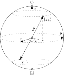
Figure 2: Berry phases in Bloch space (or the entanglement space). The parameter $\theta$ comes from the Yang–Baxterization of the unitary braiding operators, while parameters $\varphi$ originates from the $q$-deformation of the braiding operators. They define a point on the unit three-dimensional sphere named the Bloch sphere, and have definite geometric meanings as angles of longitude and latitude respectively. Let $\theta$ be time-independent, when the parameter $\varphi(t)$ evolves adiabatically from 0 to $2\pi$, one obtains the Berry phases for $\chi_{\pm}(\theta,\varphi)$ as shown in Eq. (24). The relation between Berry phases and concurrence of the entangled states $\chi_{\pm}(\theta,\varphi)$ is $\gamma_{\pm}=\mp\pi(1-\sqrt{1-{\cal C}^{2}})$, where ${\cal C}=|\sin\theta|$ is the concurrence.

Actually, the eigenstates $|\chi_{\pm}(\theta,\varphi)\rangle$ are the $SU(2)$ spin coherent states. If we express the Hamiltonian in terms of $SU(2)$ generators as 87CSS

$$H(\theta,\varphi)=X_{1}J_{1}+X_{2}J_{2}+X_{3}J_{3},$$ (25)

where $X_{1}=2\hbar{\dot{\varphi}}\cos\theta\sin\theta\cos\varphi$, $X_{2}=2\hbar{\dot{\varphi}}\cos\theta\sin\theta\sin\varphi$, $X_{3}=2\hbar{\dot{\varphi}}\cos\theta\cos\theta$, and the $SU(2)$ generators are

$$J_{1}=(S^{+}_{i}\otimes S^{+}_{i+1}+S^{-}_{i}\otimes S^{-}_{i+1})/2,$$

$$J_{2}=(S^{+}_{i}\otimes S^{+}_{i+1}-S^{-}_{i}\otimes S^{-}_{i+1})/{2i},$$

$$J_{3}=(S^{z}_{i}\otimes{\bf 1}_{i+1}+{\bf 1}_{i}\otimes S^{z}_{i+1})/2,$$ (26)

based on which one can verify directly that

$$|\chi_{+}(\theta,\varphi)\rangle=\exp[\zeta J_{+}-\zeta^{*}J_{-}]\;|00\rangle,$$

$$|\chi_{-}(\theta,\varphi)\rangle=\exp[\zeta J_{+}-\zeta^{*}J_{-}]\;|11\rangle,$$ (27)

where $\exp[\zeta J_{+}-\zeta^{*}J_{-}]$ is the spin coherence operators (and also the usual $D^{\frac{1}{2}}(\theta,\varphi)$-matrix in the angular momentum theory), $J_{\pm}=J_{1}\pm iJ_{2}$ and $\zeta=e^{-i\varphi}\theta/2$. Berry phase for spin coherence states has been discussed in 87CSS , where the corresponding result coincides with Eq. (24).

IV Conclusion and Discussion

In summary, we have shown that braiding transformation is a natural approach to describe quantum entanglement, by applying the unitary braiding operators to realize entanglement swapping and to generate the GHZ states as well as the linear cluster states. The unitary braiding matrix $B_{i,i+1}$ describes the Bell states and the Yang–Baxter matrix $\check{R}_{i,i+1}(\theta,\varphi)$ describes generally entangled states with arbitrary degree of entanglement. Varying the parameter $\theta$ continuously from 0 to $2\pi$, one may obtain an “oscillating entanglement” phenomenon for the entangled states. A Hamiltonian is constructed from the unitary $\check{R}_{i,i+1}(\theta,\varphi)$-matrix, where $\varphi=\omega t$ is time-dependent while $\theta$ is time-independent. This in turn allows us to investigate the Berry phases for the entangled states in the entanglement space.

Let us make two discussions to end this paper.

(i) Very recently, geometric phases for mixed states Sjoqvist have been observed in experiments by using NMR interferometry Du as well as single photon interferometry Ericsson . Under a certain noisy environment, the states $|\chi_{\pm}(\theta,\varphi)\rangle$ may become mixed states as

$$\rho_{\pm}(r,\theta,\varphi) = r\;|\chi_{\pm}\rangle\langle\chi_{\pm}|+(1-r)\rho_{\rm noise},$$ (28)

where $0\leq r\leq 1$. Usually, $\rho_{\rm noise}$ is chosen as ${\bf 1}_{i}\otimes{\bf 1}_{i+1}/4=(|00\rangle\langle 00|+|01\rangle\langle 01|+|10\rangle\langle 10|+|11\rangle\langle 11|)/4$ and $\rho_{\pm}(r,\theta,\varphi)$ become the generalized Werner states Niels . Following Ref. Singh , one may calculate the geometric phases for the mixed states $\rho_{\pm}(r,\theta,\varphi)$, however, the computation becomes complicated since $\rho_{\pm}(r,\theta,\varphi)$ have two nonzero degenerate eigenvalues in the subspace spanned by $\{|01\rangle,|10\rangle\}$. Geometric phases for degenerate mixed states are complicated and we will discuss them elsewhere. In the following, we would like to discuss a more simpler case for geometric phases of mixed states, by restricting the noise in the subspace spanned by $\{|00\rangle,|11\rangle\}$. The analysis on such a restriction to the noisy environment is limited, for it assumes that the states $|01\rangle$ and $|10\rangle$ are decoupled, and the environment only affects the $|00\rangle$ and $|11\rangle$ subspace.

For simplicity, let us denote $|\underline{0}\rangle\equiv|00\rangle$, $|\underline{1}\rangle\equiv|11\rangle$, then the Hamiltonian can be rewritten in a very simple form as $H(\theta,\varphi)=\hbar{\dot{\varphi}}\cos\theta\;\hat{\bf r}\cdot{\mathbf{\sigma}}$, where $\hat{\bf r}=(\sin\theta\cos\varphi,\sin\theta\sin\varphi,\cos\theta)$ is a unit vector on the Bloch sphere, and ${\mathbf{\sigma}}=(\sigma_{1},\sigma_{2},\sigma_{3})$ is the Pauli matrix vector in the basis of $\{|\underline{0}\rangle,|\underline{1}\rangle\}$, namely, $\sigma_{1}=|\underline{0}\rangle\langle\underline{1}|+|\underline{1}\rangle\langle\underline{0}|$, $\sigma_{2}=-i|\underline{0}\rangle\langle\underline{1}|+i|\underline{1}\rangle\langle\underline{0}|$, $\sigma_{3}=|\underline{0}\rangle\langle\underline{0}|-|\underline{1}\rangle\langle\underline{1}|$. Based on which, the pure states $|\chi_{\pm}(\theta,\varphi)\rangle$ can be rewritten in a density matrix form as $|\chi_{\pm}\rangle\langle\chi_{\pm}|=(1\!\!1\pm\hat{\bf r}\cdot{\mathbf{\sigma}})/2,$ where $1\!\!1=|\underline{0}\rangle\langle\underline{0}|+|\underline{1}\rangle\langle\underline{1}|$. In other words, in the basis of $\{|\underline{0}\rangle,|\underline{1}\rangle\}$, $|\chi_{\pm}\rangle$ may be viewed as states of a single “qubit”, which allows us to introduce mixed states and discuss their geometric phases in a particular noisy environment as follows. By choosing $\rho_{\rm noise}=1\!\!1/2$, one has from Eq. (28) that

$$\rho_{\pm}(r,\theta,\varphi)=\frac{1}{2}(1\!\!1\pm{\bf r}\cdot{\mathbf{\sigma}}),$$ (29)

where ${\bf r}=r\hat{\bf r}$. The state $|\chi_{+}\rangle$ corresponds to a point $\hat{\bf r}$ on the Bloch sphere; $\rho_{\rm noise}$ is located on the center of the Bloch sphere; the unit vector $\hat{\bf r}$ shrinks to ${\bf r}$ when the particular noise is presented and then $|\chi_{\pm}\rangle\langle\chi_{\pm}|$ turn to be mixed states $\rho_{\pm}(r,\theta,\varphi)$. Follow the same calculations in Singh , let $r$ and $\theta$ be time-independent, when parameter $\varphi(t)$ evolves adiabatically from 0 to $2\pi$, one obtains the geometric phase for the mixed states (29) as

$$\gamma_{\pm}^{\rm mixed} = \mp\arctan(r\tan\frac{\Omega}{2}),$$ (30)

which reduces to Eq. (24) for $r=1$.

(ii) The Berry phases in Eq. (24) can be expressed in terms of the concurrence of the states $|\chi_{\pm}(\theta,\varphi)\rangle$ as $\gamma_{\pm}=\mp\pi(1-\sqrt{1-{\cal C}^{2}})$, with ${\cal C}=|\sin\theta|$ being the concurrence. It is well-known that ${\cal C}$ is an invariant of entanglement for the entangled states $|\chi_{\pm}(\theta,\varphi)\rangle$, while Berry phase is related to some certain topological structures. This might bridge a connection between quantum entanglement and topological quantum computation. Eventually, when one restricts the discussion to the basis of $\{|\underline{0}\rangle,|\underline{1}\rangle\}$, by taking $\theta=\pi/4$, $\phi=-\pi/2$ (or $q=i$), the matrix $\check{R}_{i,i+1}$ may reduce to the two-dimensional representation of braiding operators as in Eq. (140) of Slingerland , which has physical applications in non-Abelian quantum Hall systems and topological quantum field theory.

ACKNOWLEDGMENTS The authors thank Prof. L. D. Faddeev and Prof. K. Fijikawa for their encouragement and useful discussions. This work was supported in part by NSF of China (Grant No. 10575053 and No. 10605013) and Program for New Century Excellent Talents in University.

References

• (1) A. K. Ekert, Phys. Rev. Lett. 67, 661 (1991).
• (2) C. H. Bennett, and S. J. Wiesner, Phys. Rev. Lett. 69, 2881 (1992); C. H. Bennett, G. Brassard, C. Crépeau, R. Jozsa, A. Peres, and W. K. Wootters, Phys. Rev. Lett. 70, 1895 (1993).
• (3) M. A. Nielsen and I. L. Chuang, Quantum Computation and Quantum Information (Cambridge University Press, 2000).
• (4) C. H. Bennett, D. P. DiVincenzo, J. A. Smolin, and W. K. Wootters, Phys. Rev. A 54, 3824 (1996).
• (5) L. H. Kauffman and S. J. Lomonaco Jr., New J. Phys. 6, 134 (2004); J. M. Franko, E. C. Rowell, and Z. Wang, J. Knot Theory Ramifications 15, 413 (2006).
• (6) Y. Zhang, L. H. Kauffman and M. L. Ge, Int. J. Quant. Inform. 3, 669 (2005).
• (7) A. Y. Kitaev, Annals Phys. 303, 2 (2003); e-print quant-ph/9707021.
• (8) Yang–Baxter Equations in Integrable Systems, edited by M. Jimbo (World Scientific, Singapore, 1990).
• (9) J. K. Slingerland, and F. A. Bais, Nucl. Phys. B 612, 229 (2001).
• (10) G. Badurek, H. Rauch, A.Zeilinger, W. Bauspiess, and U. Bonse, Phys.Rev. D 14, 1177 (1976); A. Zeilinger, Physica B 137, 235 (1986).
• (11) M. Żukowski, A. Zeilinger, M. A. Horne, and A. K. Ekert, Phys. Rev. Lett. 71, 4287 (1993).
• (12) A. Zeilinger, M. A. Horne, H. Weinfurter, and M. Żukowski, Phys. Rev. Lett. 78, 3031 (1997).
• (13) S. Bose, V. Vedral, and P. L. Knight, Phys. Rev. A 57, 822 (1998).
• (14) J. W. Pan, D. Bouwmeester, H. Weinfurter, A. Zeilinger, Phys. Rev. Lett. 80, 3891 (1998).
• (15) R. Raussendorf and H. J. Briegel, Phys. Rev. Lett. 86, 5188 (2001).
• (16) R. Prevedel, P. Walther, F. Tiefenbacher, P. Böhi, R. Kaltenbaek, T. Jennewein, and A. Zeilinger, Nature 445, 65 (2007).
• (17) W. K. Wootters, Phys. Rev. Lett. 80, 2245 (1998).
• (18) Geometric Phases in Physics, edited by A. Shapere and F. Wilczek (World Scientific, Singapore, 1989).
• (19) S. Chaturvedi, M. S. Sriram, and V. Srinivasan, J. Phys. A 20, L1091 (1987).
• (20) E. Sjöqvist, A. K. Pati, A. Ekert, J. S. Anandan, M. Ericsson, D. K. L. Oi, and V. Vedral, Phys. Rev. Lett. 85, 2845 (2000).
• (21) J. Du, P. Zou, M. Shi, L. C. Kwek, J. W. Pan, C. H. Oh, A. Ekert, D. K. L. Oi, and M. Ericsson, Phys. Rev. Lett. 91, 100403 (2003).
• (22) M. Ericsson, D. Achilles, J. T. Barreiro, D. Branning, N. A. Peters, and P. G. Kwiat, Phys. Rev. Lett. 94, 050401 (2005).
• (23) K. Singh, D. M. Tong, K. Basu, J. L. Chen, and J. F. Du, Phys. Rev. A 67, 032106 (2003).