Fluctuations in glassy systems

Abstract

We summarize a theoretical framework based on global time-reparametrization invariance that explains the origin of dynamic fluctuations in glassy systems. We introduce the main ideas without getting into much technical details. We describe a number of consequences arising from this scenario that can be tested numerically and experimentally distinguishing those that can also be explained by other mechanisms from the ones that we believe, are special to our proposal. We support our claims by presenting some numerical checks performed on the $3d$ Edwards-Anderson spin-glass. Finally, we discuss up to which extent these ideas apply to super-cooled liquids that have been studied in much more detail up to present.

1 Why glasses? vs. universality in glassy dynamics

It is common to encounter in nature systems that resist equilibration with their environments and display what is called glassiness. The name is derived from what we normally know as glasses, an irregular array of silicon and oxygen atoms without crystalline order, much as a liquid, but as hard as a solid. The molecular diffusion within glasses is extremely sluggish, slowing down by over 10 orders of magnitude as the temperature is slightly decreased near the operationally defined glass transition temperature. Hence, the term glassiness became generically associated with very slow dynamics [1].

So, why glasses? The answer to this question has been the focus of much research effort for long. It is certainly a rather difficult question, and there have been a number of ideas lined up for trying to understand how material systems become glassy. It is not even clear whether in many systems there is a thermodynamic phase one can call glass, or there is simply a dynamical crossover at low enough temperatures.

Do we need to fully answer why glasses? before we really further our understanding of glassy dynamics? We take the point of view that, by starting from the fact that glassy systems exist (as nature presents us with concrete examples), we can then attempt to characterize whatever possible universal properties there are in glassy dynamics.

To make this statement clearer, let us turn to a question that Anderson poses in the introduction of his Concepts in solids text [2]: why solids? This question, again, is a rather complex one, and it is not untwined from the question why glasses? if we focus on why a regular array of atoms, as opposed to a random packing, forms in the first place. Even if one assumes that a crystalline structure forms at low temperatures, a detailed quantitative analysis of the energetics remains to be done so as to determine if the packing is hexagonal, cubic, body or face centered, etc. Nonetheless, if one starts from the existence (as observed in nature) of a state with broken translational symmetry, one can construct theories of lattice vibrations (and quantize it) and of electronic band structure (and discern between insulators, metals and semiconductors). Solid state physics starts from the solid.

The approach we review in this paper relies on a similar philosophy: we do not claim any theory of the glass transition, and we do not attempt to answer why glasses? with this particular approach. Our theory does not allow us to make non-universal predictions, such as what the glass transition temperature is (if one can be defined) for a certain material, or whether the material displays glassy behavior at all. We aim at understanding if there is a set of principles, guided by symmetry considerations, that can be used to understand certain universal aspects of glassy dynamics once the glass state is presented. For example, glasses age [3]. We thus expect that there exists a unified approach to describe aging phenomena, and we seek some guiding principles, based on dynamical symmetries, that could allow us to understand universal properties in the aging regime, including the scaling of spatial heterogeneities.

We propose that the symmetry that captures the universal aging dynamics of glassy systems is the invariance of an effective dynamical action under uniform reparametrizations of the time scales [4]-[9]. Such type of invariance had been known to exist since the early days in which the mean-field equilibrium dynamics of spin-glasses was tried to be understood [10, 11] and it was later encountered in the better formulated out of equilibrium dynamic formalism applied to the same systems [12, 13]. The invariance means that in the asymptotic regime of very long times a family of solutions to the equations of motion is found. This ‘annoyance’, we claim, has actually a physical meaning and implications in the fluctuating dynamics of real glasses. In order to make this statement concrete, it is necessary to show that the invariance also exists in finite dimensional glassy models. With this aim we showed that global time reparametrization invariance emerges in the long times action of short-range spin-glasses assuming causality and a separation of time scales [4]-[6]. Basically, the second assumption amounts to start from a glass state, where one may claim there is a separation between, roughly, a time regime where relaxation is fast and another where relaxation is slow. The invariance can then be used to describe dynamic fluctuations in spin-glasses and, we conjectured, in other glassy systems as well.

Physically, the emergence of time reparametrization invariance can be though of in the following way. The out of equilibrium relaxation of glassy systems is well characterized by two-time functions, either correlations or linear responses. In the slow and aging regime they depend on two times and time-translation invariance is lost. The proper measure of ‘time’ inside the system is the value of the correlation itself, and not the ‘wall clock’ in the laboratory. For instance, in a spin-glass the proper measure of sample age is the spin-spin overlap or in particle systems it is the incoherent correlation function. Age measures can fluctuate from point to point in the sample, what we called heterogeneous aging, with younger and older pieces (lower and higher values of the correlation) coexisting at the same values of the two laboratory times. The fact that the effective dynamical action becomes invariant under global time reparametrizations, $t\to h(t)$, everywhere in the sample, means that the action weights the fluctuations of the proper ages, $C({\vec{r}};t_{1},t_{2})$, directly, and the times $t_{1}$ and $t_{2}$ in the action are just integrated over as dummy variables. To draw an analogy, in theories of quantum gravity the space-time variables $X_{\mu}(\tau,\sigma)$ are the proper variables, and the action is invariant under conformal transformations of the world-sheet parameters $\tau$ and $\sigma$.

So what does global time-reparametrization invariance symmetry concretely teach us about observables in glasses? So far we discussed a global symmetry or invariance with respect to uniform time-reparametrizations. By looking at spatially heterogeneous reparametrizations, we can predict the behavior of local correlations and linear susceptibilities and the relations between them. For example, we predict that, after a convenient normalization that we explain in the main text, the triangular relation between the local coarse-grained correlations, $C(\vec{r};t_{1},t_{2})$, $C(\vec{r};t_{2},t_{3})$ and $C(\vec{r};t_{1},t_{3})$, as a function of the intermediate time $t_{2}$, $t_{3}<t_{2}<t_{1}$, at all spatial points, $\vec{r}$, should be identical to the global triangular relation, in the asymptotic limit of very long absolute times and delays between them and very large coarse-graining linear length [9]. Different sites can be retarded or advanced with respect to the global behaviour but they should all have the same overall type of decay. Similarly, the relation between local susceptibilities and their associated correlations should be identical all over the sample [5, 6] leading to a uniform effective temperature [14].

The purpose of this article is to describe our current understanding of dynamic fluctuations (heterogeneities) in the non-equilibrium relaxation of glassy systems arising from the time-reparametrization invariance scenario [4]-[9],[15]. We illustrate it by presenting critical tests.

The structure of this review is the following. In Sect. 2 we explain the origin of the time-reparametrization invariance scenario. We do not present detailed derivations that were already published but we aim at highlighting the main ideas behind the scene. In Sect. 3 we list several measurable consequences of the theory. We discuss how they have been examined numerically in different glassy models. The discuss here which consequences could also be explained by other approaches and which, we believe, are unique to our scenario. Finally, in Sect. 4 we discuss the scenario. Since this research project is not closed yet, we present some proposals for numeric and experimental tests as well as some ideas about analytic calculations that could help us understanding the limitations of our proposal.

2 Time reparametrization invariance

In this Section we explain how global time-reparametrization invariance develops asymptotically in the aging regime of glassy models. For the sake of simplicity we focus on the classical formalism and at the end of this section we mention the modifications introduced by quantum fluctuations.

2.1 Mean-field models – dynamic equations

Schematic models of spin-glasses, structural glasses and ferromagnetic clean coarsening are encoded in the family of $p$-spin models defined by [16]

$$H=-\sum_{i_{1}i_{2}\dots i_{p}}J_{i_{1}i_{2}\dots i_{p}}s_{i_{1}}s_{i_{2}}\dots s_{i_{p}}$$ (1)

with quenched disordered exchanges distributed with the Gaussian law $P(J_{i_{1}i_{2}\dots i_{p}})\propto e^{-p!\,J_{i_{1}i_{2}\dots i_{p}}^{2}/(2N^{p-1})}$. The dynamic variables $s_{i}$, $i=1,\dots,N$, are of Ising type, $s_{i}=\pm 1$, or satisfy a global spherical constraint $\sum_{i=1}^{N}s_{i}^{2}=N$. $p$ is an integer parameter: with $p=2$ and Ising variables one mimics spin-glasses, with $p>2$ and Ising or spherical spins the phenomenology of structural glasses is recovered, and with $p=2$ and spherical spins one describes ferromagnetic domain-growth in clean systems. The sum runs over all $p$-uplets; for this reason these models are ‘mean-field’ in the sense that the saddle-point evaluation of the partition function or the dynamic generating functional is exact in the thermodynamic limit, $N\to\infty$. The Hamiltonian (1) also represents the potential energy of a particle with position $\vec{s}=(s_{1},\dots,s_{N})$ on an infinite dimensional hypercube ($s_{i}=\pm 1$) or hypersphere ($\sum_{i=1}^{N}s_{i}^{2}=N$).

Dynamics is introduced with a Langevin equation that represents the coupling of the spins to an equilibrated thermal environment. Ising spins are then replaced by soft variables by introducing a double-well potential energy, $\sum_{i=1}^{N}V(s_{i})$, with $V(s_{i})=a(s_{i}^{2}-1)^{2}$. The initial condition is usually chosen to be random thus mimicking a rapid quench from infinite temperature to the working temperature $T$. In the limit $N\to\infty$ exact Schwinger-Dyson equations couple the global correlation and instantaneous linear response

$$NC(t,t_{w})=\sum_{i=1}^{N}s_{i}(t)s_{i}(t_{w})\;,\qquad NR(t,t_{w})=\sum_{i=1}^{N}\left.\frac{\delta s_{i}(t)}{\delta h_{i}(t_{w})}\right|_{h=0}\;$$ (2)

($\sum_{i=1}^{N}s_{i}(t)=0$ for all $t$). The field $h_{i}$ couples linearly to the spin variables and, in general, we are interested in perturbing fields that are uncorrelated with the equilibrium states of the systems. It is not necessary to average over thermal noise or quenched disorder since these quantities do not fluctuate in the out of equilibrium regime reached when the infinite volume limit ($N\to\infty$) has been taken at the outset. Here are in what follows times are measured from an origin that corresponds to the quench to the working temperature. Our study applies then in the order of limits

$$\lim_{t_{w}\to\infty}\lim_{N\to\infty}$$ (3)

in which the exact causal Schwinger-Dyson equations for spherical models at times $t\geq t_{w}$ read [12, 19]

$$(\partial_{t}-z_{t})C(t,t_{w})=\int_{0}^{t}dt^{\prime}\;\Sigma(t,t^{\prime})C(t^{\prime},t_{w})+\int_{0}^{t_{w}}dt^{\prime}\;D(t,t^{\prime})R(t_{w},t^{\prime})\;,$$ (4)

$$(\partial_{t}-z_{t})R(t,t_{w})=\int_{t_{w}}^{t}dt^{\prime}\;\Sigma(t,t^{\prime})R(t^{\prime},t_{w})+\delta(t-t_{w})\;,$$ (5)

where the vertex, $D$, and self-energy, $\Sigma$, are functions of $C$ and $R$

$$D(t,t_{w})=\frac{p}{2}C^{p-1}(t,t_{w})\;,\;\;\;\;\;\;\Sigma(t,t_{w})=\frac{p(p-1)}{2}C^{p-2}(t,t_{w})\,R(t,t_{w})\;.$$ (6)

The Lagrange multiplier $z_{t}$ is fixed by requiring $C(t,t)=1$. For Ising problems the soft spin constraint can be treated in the mode-coupling approximation [17] or else, one can apply a $T-T_{c}$ expansion taking advantage of the fact that the phase transition is of second order for $p=2$ (Sherrington-Kirkpatrick or SK model) [13].

In such fully-connected models all higher order correlations and linear responses factorize and can be written as functions of these two-time functions. Self-consistent approximate treatments of interacting particle models with realistic potentials, like the mode-coupling approach, yield similar equations with the addition of a wave-vector dependence that in the present context can also be taken into account by considering models of $d$-dimensional random manifolds embedded in $N\to\infty$ dimensional spaces [18, 19].

2.2 Structural glasses: the $p\geq 3$ cases

We now focus on the $p\geq 3$ cases that mimic the structural glass problem. We mention at the end of this subsection the Ising $p=2$ (SK) spin-glass case that is not conceptually different but just technically more involved. In Sect. 2.5 we discuss the $p=2$ spherical problem that yields a mean-field description of coarsening phenomena and is rather different from the point of view of time-reparametrization transformations.

Equations (4) and (5 are causal and be solved numerically by constructing $C(t,t_{w})$ and $R(t,t_{w})$ from the initial instant $t=t_{w}=0$. An analytic solution is possible in the asymptotic limit, as we discuss below. We first present the main features of $C$ and $R$ and we later explain how these are obtained from the asymptotic analytic solution.

Equations (4) and (5) have a dynamic transition at a critical temperature $T_{d}(p)$. At $T>T_{d}$ the dynamics occurs in equilibrium and close to $T_{d}$ the decay of the correlations slows down as in super-cooled liquids with the $\alpha$ relaxation time diverging as a power law of $T-T_{d}$ [16, 20]. Below $T_{d}$ eqs. (4) and (5) admit a unique solution [12, 13] that is no longer stationary. The behaviour of the low-temperature correlation and susceptibility is sketched in Fig. 1.

The low-temperature solution presents a separation of time-scales. In the long waiting-time limit the self-correlation and integrated linear response or susceptibility, $\chi(t,t_{w})\equiv\int_{t_{w}}^{t}dt^{\prime}\,R(t,t^{\prime})$, can be written as

$$C(t,t_{w}) = C_{st}(t-t_{w})+C_{ag}(t,t_{w})\;,$$ (7)

$$\chi(t,t_{w}) = \chi_{st}(t-t_{w})+\chi_{ag}(t,t_{w})\;.$$ (8)

The first terms in the right-hand-side describe the stationary regime at short time-differences in which the correlation and susceptibility relatively rapidly approach a plateau at $\lim_{t-t_{w}\to\infty}\lim_{t_{w}\to\infty}C(t,t_{w})=q_{ea}$ and $\lim_{t-t_{w}\to\infty}\lim_{t_{w}\to\infty}\chi(t,t_{w})=(1-q_{ea})/T\equiv\chi_{ea}$. The second terms are the aging relaxation of $C$ towards zero (in the absence of an external field), and the aging response of the system towards the asymptotic value $\chi_{ea}+q_{ea}/T_{eff}$ with $T_{eff}$ a parameter with the interpretation of an effective temperature [14].

Figure 1: Sketch of the relaxation of the self-correlation and susceptibility in the glassy regime. The separation of time-scales is clear in the figure. The Edwards-Anderson parameter, $q_{ea}$ the corresponding susceptibility $\chi_{ea}$ and the asymptotic value $\lim_{t\to\infty}\chi(t,t_{w})$ are indicated with horizontal lines.

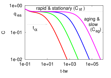
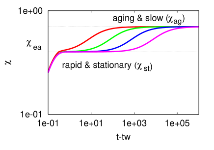
The stationary and aging relaxation are fast and slow in the sense that

$$\partial_{t}C_{st}(t,t_{w})\sim C_{st}(t,t_{w}) \qquad\qquad\qquad C>q_{ea}\;,$$ (9)

$$\partial_{t}C_{ag}(t,t_{w})\ll C_{ag}(t,t_{w}) \qquad\qquad\qquad C<q_{ea}\;,$$ (10)

and

$$\partial_{t}\chi_{st}(t,t_{w})\sim\chi_{st}(t,t_{w}) \qquad\qquad\qquad\chi<\chi_{ea}\;,$$ (11)

$$\partial_{t}\chi_{ag}(t,t_{w})\ll\chi_{ag}(t,t_{w}) \qquad\qquad\qquad\chi>\chi_{ea}\;.$$ (12)

The aging self-correlation and susceptibility scale as

$$C_{ag}(t,t_{w})\approx q_{ea}\;f_{\sc c}\left(\frac{{\cal R}(t)}{{\cal R}(t_{w})}\right)\;,\qquad\chi_{ag}(t,t_{w})\approx q_{ea}\;f_{\chi}\left(\frac{{\cal R}(t)}{{\cal R}(t_{w})}\right)\;.$$ (13)

The scaling functions satisfy the limit conditions $f_{c}(1)=1$, $f_{c}(\infty)=0$, $f_{\chi}(1)=0$ and $f_{\chi}(\infty)=1/T_{eff}$. Using mathematical properties of monotonic two-time functions one can show that such a scaling holds asymptotically in each (two) time-scale of the evolution [13]. While in a system undergoing finite dimensional coarsening ${\cal R}(t)$ has a natural interpretation as the typical domain radius, in mean-field models there is no immediate understanding of the ‘clock’ ${\cal R}(t)$ that, in a sense, sets the macroscopic time-scale. The numerical solution suggests that ${\cal R}(t)$ is just a power of time.

In the asymptotic limit in which the additive separation of time-scales with the scaling form (13) holds it is convenient to use a parametric description of the dynamics in which times do not appear explicitly. More precisely, the approach to the asymptotic scaling, and $f_{c}$ and $f_{\chi}$, can be put to the test by constructing ‘triangular relations’ between correlations and susceptibilities, respectively. For generic three long times $t_{1}\geq t_{2}\geq t_{3}\gg t_{0}$ one computes the correlations $C(t_{\mu},t_{\nu})$, $\mu>\nu=1,2,3$. If the times are such that the ratios ${\cal R}(t_{\mu})/{\cal R}(t_{\nu})$ remain finite in the asymptotic limit, that is to say $C(t_{\mu},t_{\nu})=C_{ag}(t_{\mu},t_{\nu})$, one has

$$C(t_{1},t_{3})=q_{ea}\;f_{c}\left\{f^{-1}_{c}[C(t_{1},t_{2})/q_{ea}]\;f^{-1}_{c}[C(t_{2},t_{3})/q_{ea}]\right\}\;.$$ (14)

If, instead, $t_{1}=t_{2}+\tau$ with $\tau>0$ finite, and ${\cal R}(t_{2})/{\cal R}(t_{3})$ finite in such a way that $C(t_{1},t_{2})=q_{ea}+C_{st}(t_{1}-t_{2})$ and $C(t_{2},t_{3})=C_{ag}(t_{2},t_{3})$ one has

$$C(t_{1},t_{3})=\min\left[\,C(t_{1},t_{2}),C(t_{2},t_{3})\,\right]$$ (15)

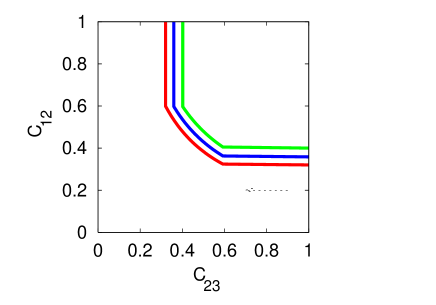
asymptotically. This form goes under the name of dynamic ultrametricity. In the opposite case $t_{3}=t_{2}-\tau$ and ${\cal R}(t_{1})/{\cal R}(t_{2})$ finite dynamic ultrametricity also holds. These relations follow immediately from the additive separation of time-scales (8) and the scaling (13) but they can be shown without assuming dynamic scaling, just by using the monotonicity properties of temporal correlations [13]. The simplest way to see these relations at work is to display $C(t_{1},t_{2})$ against $C(t_{2},t_{3})$, for a chosen value of $C(t_{1},t_{3})<q_{ea}$, in a parametric plot in which $t_{2}$ varies from $t_{3}$ to $t_{1}$. In the asymptotic limit $t_{3}\to\infty$ the construction reaches a stable master curve as displayed in Fig. 2-left. The vertical and horizontal parts correspond to $t_{2}$ such that $C(t_{1},t_{2})>q_{ea}$ and $C(t_{2},t_{3})>q_{ea}$, respectively, and dynamic ultrametricity holds. The curved part is for $t_{2}$ such that all correlations are in the aging regime and its functional form is fully determined by $f_{c}$. The ‘clock’ ${\cal R}$ yields the speed at which the data-point moves on the parametric curve. A similar construction can be done for the susceptibilities.

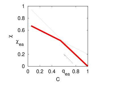
The stationary correlation, $C_{st}$, and susceptibility, $\chi_{st}$, are linked by the equilibrium fluctuation dissipation theorem (fdt), $\chi_{st}=(1-C_{st})/T$. In the aging regime, instead, there is a non-trivial relation between $\chi$ and $C$: $\chi_{ag}=(q_{ea}-C_{ag})/T_{eff}$ that yields $f_{\chi}(x)=(1-f_{c}(x))/T_{eff}$. This relation is also better appreciated if shown in a parametric construction in which times do not appear explicitly. In the long waiting-time limit the plot $\chi(t,t_{w})$ against $C(t,t_{w})$ with $t$ the parameter running from $t_{w}$ to infinity approaches a broken line form with the slopes $-1/T$ (for $C>q_{ea}$) and $-1/T_{eff}$ (for $C<q_{ea}$). Again, the ‘clock’ ${\cal R}$ yields the speed at which this curve is constructed upon increasing $t$.

                              

Figure 2: Sketch of the parametric representation of the correlation and susceptibility. Left: triangular relation between the correlation function in the asymptotic limit $t_{3}\to\infty$. The three curves correspond to different $t_{1}$’s such that $C(t_{1},t_{3})$ takes three values. The breaking points lie at $q_{ea}$. The arrow indicates the sense of the evolution when $t_{2}$ increases from $t_{3}$ to $t_{1}$. Right: susceptibility, $\chi(t_{2},t_{3})$ against correlation, $C(t_{2},t_{3})$ at fixed $t_{3}$ using $t_{2}\geq t_{3}$ as a parameter in the long $t_{3}$ limit. The breaking point at $(q_{ea},\chi_{ea})$ separates the stationary regime where the equilibrium fdt is satisfied from the aging regime where it is modified. The slopes are $-1/T$ and $-1/T_{eff}$, respectively. The arrow also indicates here the sense of the evolution when $t_{2}$ increases from $t_{3}$.

An analytic solution to the Schwinger-Dyson equations was derived in the limit of long waiting-time in which the separation of time-scales, that is to say the plateaus in $C$ and $\chi$, are fully established. In the aging regime, one uses the fact that the variation of the correlation and linear susceptibility are negligible with respect to all terms in the right-hand-side of the equations and can thus be dropped. Furthermore, one approximates the integrals by separating the contributions from the stationary and aging regimes [19]. Equation (5) becomes

$$\mu_{\infty}R_{ag}(t,t_{w})\sim\frac{p(p-1)}{2}\int_{t_{w}}^{t}dt^{\prime}\;C^{p-2}_{ag}(t,t^{\prime})R_{ag}(t,t^{\prime})\,R_{ag}(t^{\prime},t_{w})\;$$ (16)

($\mu_{\infty}$ is a constant with contributions from $\lim_{t\to\infty}z_{t}$ and border terms in the integrals). The companion eq. (4) takes a similar form within the same approximation. Now, the surprise is that the approximate equations are invariant under the transformation

$$t\to h_{t}\equiv h(t)\;,\qquad\qquad \left\{\begin{array}[]{l}C_{ag}(t,t_{w})\to C_{ag}(h_{t},h_{t_{w}})\;,\\ R_{ag}(t,t_{w})\to\dot{h}_{t_{w}}\,R_{ag}(h_{t},h_{t_{w}})\;,\end{array}\right.$$ (19)

with $h_{t}$ positive and monotonic and $\dot{h}_{t_{w}}\equiv dh_{t_{w}}/dt_{w}$. While the functions $f_{c}$ and $f_{\chi}$ and their fd relation are fixed by the remaining approximate equation (16) and its companion, the time-reparametrization invariance does not allow one to compute, analytically, the clock ${\cal R}(t)$. This problem is similar to the velocity selection problem present for instance in Fisher differential equation describing front propagation and the like [21]. The exact Schwinger-Dyson equations do have a unique solution with a special function ${\cal R}(t)$ that is selected by the short-time difference effect of the time-derivatives. However, as time increases and time-differences increase too the effect of the time-derivatives diminishes. In the approximate analytic solution we take advantage of this fact to solve the equations asymptotically but we introduce in this way a symmetry that does not allow us to fix ${\cal R}(t)$. We obtain, instead, a family of solutions parametrized by $h_{t}$. It is important to reckon that the parametric constructions in Fig. 2 are independent of the clock and thus are fully determined by the approximate treatment.

The case $p=2$ with Ising spins or Sherrington-Kirkpatrick model has a more complicated scaling form with a sequence of two-time scales leading to dynamic ultrametricity for all $C<q_{ea}$ asymptotically [13]. This behaviour is technically more involved but, as far as the symmetry properties are concerned, it is similar to the case treated above. The full dynamic equations have a unique solution but the approximate ones acquire time-reparametrization invariance. We shall not discuss these cases further in the rest of this review.

2.3 Short-ranged models – dynamic action

In a series of papers [4]-[9] we claimed that the time-reparametrization invariance thus far introduced via the asymptotic solution to the dynamic equations in mean-field glassy problems is indeed an asymptotic property of the dynamics of glassy systems, mean-field and finite dimensional. The separation of time-scales stationary-aging has been observed in a variety of glassy systems with numerical simulations and experiments [3, 22]. The slowness of the decay in the aging regime, eqs. (10) and (12) and a weak long-term memory of the kind (13), are the hallmark of glassy relaxation. The idea is then that time-reparametrization invariance is the symmetry associated to the dominant dynamic fluctuations in these sytems.

In order to pursue this idea forward one has to first prove that the symmetry of the saddle-point equations is also a symmetry of the action in the dynamic generating functional not only of fully-connected spin models of the mean-field type but also of finite dimensional glassy systems. In [4] we derived and studied the symmetry properties of the dynamic action – the so-called Martin-Siggia-Rose action associated to Langevin stochastic dynamics – of the disorder averaged soft-spin $3d$ Edwards-Anderson (ea) model of spin-glasses. ($H=\sum_{\langle ij\rangle}J_{ij}s_{i}s_{j}$ with $J_{ij}$ Gaussian random variables with zero mean and taking non-zero value only on nearest neighbours on the $d$-dimensional lattice and $s_{i}=\pm 1$.) In our analysis we took a number of steps that we briefly recall here. First, we introduced four fluctuating two-time fields defined on the lattice sites,

$$Q^{ab}_{i}(t,t_{w})\;,\qquad\mbox{with}\qquad i=1,\dots,N\;\;\mbox{and}\;\;a,b=0,\,1\;.$$ (20)

Their thermal averages are the expected values of the local two-time self-correlation ($a=b=0$), the retarded linear response ($a=0$, $b=1$), the advanced linear response ($a=1$, $b=0$), and a fourth observable ($a=b=1$) that vanishes if causality is preserved. Second, we assumed that a separation of time-scales fast-slow, of the type described in the previous subsection, applies to these fluctuating fields too. Third, we determined the long-time action by using a Renormalization Group (RG) scheme in the time variables. This allowed us to write the full action as a sum of two contributions: one from the fast regime holding at short time-differences, another one from the slow regime valid at long time-differences. The coupling between these two vanishes asymptotically. Fourth, we analyzed the surviving terms in the action, that are just the slow contribution. Using advanced and retarded scaling dimensions that are just the labels $a$ and $b$ of the fields, one finds that the global time-reparametrization,

$$t\to h_{t}\equiv h(t)\;,\qquad\qquad{{\widetilde{Q}}_{i}^{ab}}(t,t_{w})=(\dot{h}_{t})^{a}(\dot{h}_{t_{w}})^{b}\;Q_{i}^{ab}(h_{t},h_{t_{w}})\;,$$ (21)

leaves all surviving terms unmodified. This step is concisely carried out as follows. Take a generic term in the action. Under (21) it transforms as

$$\int\prod_{\nu=1}^{\cal N}dt_{\nu}\;\cdots \to \int\prod_{\nu=1}^{\cal N}dt_{\nu}\;(\dot{h}_{t_{\nu}})^{\Delta_{\nu}}\;\cdots$$

where ${\cal N}$ is the number of time integrals, the dots represent a product of the fields $Q_{i}^{ab}$ and $\Delta_{\nu}$ is the sum of all factors $\dot{h}_{t_{\nu}}$ arising from the transformation of the fields. Interestingly enough, one finds that all the $\Delta_{\nu}$ equal one. Thus, with a simple change of variables one absorbs each factor $\dot{h}_{t_{\nu}}$ in the corresponding integration variable and

$$\int\prod_{\nu=1}^{\cal N}dt_{\nu}\;\cdots\to\int\prod_{\nu=1}^{\cal N}dh_{\nu}\;\cdots$$ (22)

Note that in order to prove invariance under the simpler and more common scale transformation, $h_{t}=\lambda t$, it is enough to have $\sum_{\nu=1}^{\cal N}\Delta_{\nu}={\cal N}$. Scale invariance is included in the larger global time-reparametrization symmetry but it is, clearly, more restrictive. Finally, we showed that the measure in the functional integral is also global time-reparametrization invariant, completing the program. We refer the reader to Refs. [4] and [6] for the technical details leading to these results.

In the disordered 3$d$ ea model studied we carried out the disorder average. The presence of quenched disorder gave us an analytic control of the theory but this does not necessarily mean that such a symmetry develops only for the long time regime of models with quenched disorder. It appears that if the essential assumptions are causality and unitarity, and a separation of time scales that takes the action to a non-trivial asymptotic state (some glassy state), then one expects the symmetry to exist for systems without quenched disorder but that are glassy nevertheless. In order to check the development of time-reparametrization invariance in problems of particles in interaction in finite dimensions one should first obtain the relevant action to work with. A good candidate for a starting point is the Dean-Kawasaki stochastic equation for the evolution of the local density [23]. The idea is then to write its dynamic generating functional and study the symmetry properties of the effective action assuming that a separation of time-scales exists. We are currently carrying out this study.

2.4 Turning a nuisance into something useful - symmetry as a guideline

The global time-reparametrization invariance implies that the action describing the long time slow dynamics of a spin-glass is basically a “geometric” random surface theory, with the $Q$’s themselves as the natural coordinates. The original two times parametrize the surface. Physical quantities, as the bulk integrated response $\chi(t_{1},t_{2})=\int_{t_{2}}^{t_{1}}dt^{\prime}\,R(t^{\prime},t_{2})$ and correlation $C(t_{1},t_{2})$ have scaling dimension zero under $t\to h(t)$ as well as their local counterparts. The emergence of this gauge-like symmetry, which may appear first as a nuisance that relates too many solutions for just one problem. However, it may provide a simple way to understand spatial fluctuations in systems that possess this global time-reparametrization symmetry.

Here, a simple analogy with the problem of a ferromagnet may elucidate the point we want to make. In a ferromagnet the action is invariant under uniform rotations of the magnetization vector $\vec{m}$. In the ordered phase, rotation symmetry is spontaneously broken, and a certain magnetization direction $\vec{m}_{0}$ is picked. Typically, a vanishingly small pinning field selects this direction. The low action excitations are the spin waves, fluctuations of the uniform, symmetry broken, state. These spin waves can be described in terms of smooth spatially fluctuating rotations around the uniform magnetization state. The spin waves, generated by using slowly varying local rotations, are the Goldstone modes of the ferromagnet.

Similarly, in the aging regime of the glassy systems, the action has a global symmetry, under uniform time-reparametrizations, $t\to h(t)$, with the fields transforming as in eq. (21). The probability weight of having certain local two-time correlation and response, the observables, should be independent of this reparametrization. After coarse-graining over a linear length $\ell$ the non-vanishing fluctuating fields are the local coarse-grained correlation ($a=b=0$) and linear response ($a=0,\,b=1$),

$$C(\vec{r};t,t_{w})=\left(\frac{a}{\ell}\right)^{d}\sum_{j\in V_{\vec{r}}}s_{j}(t)s_{j}(t_{w})\;,\;\;\;R(\vec{r};t,t_{w})=\left(\frac{a}{\ell}\right)^{d}\sum_{j\in V_{\vec{r}}}\left.\frac{\delta s_{j}(t)}{\delta h_{j}(t_{w})}\right|_{h=0}\;,$$

with the sum carried over the spins in the volume $V_{\vec{r}}=\ell^{d}$ centered at $\vec{r}$, and $a$ is the lattice spacing. The transformation (19) is now restated as

$$t\to h_{t}\equiv h(t)\;,\qquad \left\{\begin{array}[]{l}C_{ag}(\vec{r};t,t_{w})\to C_{ag}(\vec{r};h_{t},h_{t_{w}})\;,\\ R_{ag}(\vec{r};t,t_{w})\to\dot{h}_{t_{w}}\,R_{ag}(\vec{r};h_{t},h_{t_{w}})\end{array},\right.$$ (25)

and it is an asymptotic symmetry of the action for the slow coarse-grained degrees of freedom. Indeed, the symmetry breaking terms, that have their origin in the short-time dynamics and short-time difference dynamics, are not identical to zero but become vanishing small asymptotically. The particular scaling function ${\cal R}(t)$ selected by the system is determined by matching the fast and the slow dynamics. It depends on several details – the existence of external forcing, the nature of the microscopic interactions, etc. In other words, the fast modes which are absent in the slow dynamics act as symmetry breaking fields for the slow modes.

In analogy with the spin-wave fluctuations in magnetic systems, that are dictated by the rotational symmetry, we proposed that the smooth fluctuations in the glassy phase can be obtained by studying the slow varying, position dependent reparametrizations $t\to h(\vec{r},t)$ around the one reparametrization ${\cal R}(t)$ selected by the short-time dynamics. In other words, we basically proposed that there are Goldstone modes for the glassy action which can be written as slowly varying, spatially inhomogeneous time reparametrizations. This suggests that the slow part of the coarse-grained local correlations and susceptibilities should scale as

$$C_{ag}(\vec{r};t,t_{w})\approx q_{ea}\;f_{\sc c}\left(\frac{h(\vec{r},t)}{h(\vec{r},t_{w})}\right)\;,\qquad{\chi_{ag}}(\vec{r};t,t_{w})\sim f_{\chi}\left(\frac{h(\vec{r},t)}{h(\vec{r},t_{w})}\right)\;,$$ (26)

with $f_{c}$ and $f_{\chi}$ the same functions describing the global correlation and susceptibility, respectively [eqs. (13) and (27)] and the same function $h(\vec{r},t)$ scaling the two-time correlation and susceptibility on each site $\vec{r}$ [4, 5, 6]. The sum rules $C_{ag}(t,t_{w})=V^{-1}\int d^{d}r\;C_{ag}(r;t,t_{w})$ and $\chi_{ag}(t,t_{w})=V^{-1}\int d^{d}r\;\chi_{ag}(r;t,t_{w})$ apply.

The reason for this proposal is that the global reparametrization invariance in time of the dynamic action in this two-time regime leads to low action excitations (Goldstone modes) for smoothly varying spatial fluctuations in the reparametrization of time, but not in the external form of the scaling functions. As in a sigma model (for example, to describe the ferromagnet), the external functions $f_{c}$ and $f_{\chi}$ fix the manifold of states, and the local time reparametrizations correspond to fluctuations restricted to this fixed manifold of states (in the ferromagnet, the tilting of direction but not the magnitude of the magnetization vector).

2.5 The spherical $p=2$ case or mean-field domain growth

The spherical SK model ($p=2$) can be solved exactly by analyzing the Langevin equation in the basis of eigenvectors of the random matrix $J_{ij}$ [24]. While the correlation has a very similar behaviour to the one of the $p\geq 3$ cases (see Fig. 1-left), the susceptibility is quite different. One can mention that the stationary and aging regimes in the linear response are not so sharply separated in this case. If one uses an additive separation as in (8) the aging contribution to the integrated linear response, $\chi_{ag}(t,t_{w})$, vanishes asymptotically. More precisely,

$$\chi_{ag}(t,t_{w})\sim t_{w}^{-1/2}\;f_{\chi}\left(\frac{t}{t_{w}}\right)\;.$$ (27)

Importantly enough, even though the inequalities (10) and (12) are still valid, a careful inspection of all terms in the Schwinger-Dyson equations shows that they are of the same order asymptotically. Moreover, the stationary contribution to the equations in the aging regime is not just a constant: the corrections associated to the asymptotic approach to the plateau in the correlation cannot be neglected. As a result one cannot simply drop the time derivatives and the Schwinger-Dyson equations in the aging regime are not time-reparametrization invariant but just scale invariant, that is to say, they are unchanged by the transformation $t\to h(t)=\lambda t$, with $C$ and $R$ transforming as in (19) and $\lambda$ a positive constant. A similar mechanism, though even harder to prove, applies to the dynamic equations for the correlation and linear response of the non-conserved dynamics of the O($N$) ferromagnetic model in the large $N$ limit [8].

In line with what we explained above, the effective action for the slow degrees of freedom of the $p=2$ spherical model and, more generally, the $d$-dimensional ferromagnetic $O(N)$ model in the large $N$ limit, are not invariant under global time-reparametrizations but only under global rescaling of time, $t\to\lambda t$. This marks an important difference between models with a finite aging response and these quasi quadratic models with a vanishing aging response [8].

This result is important for a number of reasons: first, it suggests that the susceptibility, or even the effective temperature, might be intimately related to the symmetry properties of the dynamics and consequently of the fluctuations; second, it suggests that the mechanism for fluctuations in coarsening systems might be different from the one of other glassy problems with finite and well-defined effective temperatures. In order to justify the latter statement it remains to be checked whether the reduction of time-reparametrization invariance to just scale invariance also holds in finite dimensional non-field coarsening.

2.6 Quantum problems

In the case of quantum models one introduces the effect of dissipation by coupling the system to an environment represented, typically, by an infinite ensemble of quantum harmonic oscillators. One then uses the Schwinger-Keldysh formalism to write a generating functional and from it, in the fully-connected or infinite dimensional cases, one derives Schwinger-Dyson equations similar to the ones above. The asymptotic analysis of these equations follows the same steps as in the classical limit [25, 17] (at least in the case of a weak coupling to the bath [26]) and the time-reparametrization invariance also applies.

The appearance of an asymptotic invariance under time-reparatrizations in the mean-field dynamic equations was related to the reparametrization invariance of the replica treatment of the statics of the same models [10, 27]. The latter remains rather abstract. Brézin and de Dominicis [27] studied the consequences of twisting the reparametrizations in the replica approach. Interestingly enough, this can be simply done in a dynamic treatment either by applying shear forces or by applying heat-baths with different inherent dynamics to different parts of the system. More precisely, using a model with open boundary conditions one could apply a thermal bath with a characteristic time-scale on one end and a different thermal bath with a different characteristic time-scale on the opposite end and see how a time-reparametrization ‘flow’ establishes in the model.

3 Consequences and tests

In this Section we discuss how one can put these ideas to the test by presenting a number of consequences of global time-reparametrization invariance that are directly measurable numerically and experimentally. The properties that we discuss explicitly are:

1. A growing dynamical correlation length.

2. Scaling of the pdf of local two-time functions.

3. Functional form of the pdf of local two-time functions.

4. Triangular relations between two-time functions.

5. Scaling relations for general multi-time functions.

6. Local fluctuation-dissipation relations.

7. Infinite susceptibilities.

In considering these predictions, we shall separate them into two distinct classes. The first class contains predictions that are consistent with other theoretical scenarios as well as with the presence of reparametrization invariance. Hence, while reparametrization invariance leads to these predictions, this class alone cannot be used to argue for the role of the symmetry over other mechanisms. The second class, on the other hand, contains predictions that are not natural within other frameworks, and to the date of this report have no obvious explanation within other frameworks. Properties 1 and 2 belong to the first class, properties 3-7 to the second. We shall present these properties in detail below.

3.1 Two-time correlation length

In equilibrium statistical models one defines the static correlation length, $\xi_{eq}$, from the spatial decay of the correlation between the fluctuations of the order parameter measured at two space points, $\langle\,[\phi(\vec{r})-\langle\,\phi(\vec{r})\,\rangle][\phi(\vec{r^{\prime}})-\langle\,\phi(\vec{r^{\prime}})\,\rangle]\,\rangle_{|\vec{r}-\vec{r^{\prime}}|=\Delta}\sim\Delta^{-d+2-\eta}\;e^{-\Delta/\xi_{eq}}$, where the angular brackets denote an average over the Gibbs-Boltzmann measure. $\xi_{eq}$ depends on temperature and, in second order phase transitions, it diverges at $T_{c}$ leaving only an algebraically decaying correlation. A dynamic equilibrium correlation length characterizes the spatial decay of equal-time correlations in the equilibrium relaxation of ‘usual’ systems. Similarly to the static case one defines $\xi(t)$ via $\langle\,[\phi(\vec{r},t)-\langle\,\phi(\vec{r},t)\,\rangle][\phi(\vec{r^{\prime}},t)-\langle\,\phi(\vec{r^{\prime}},t)\,\rangle]\,\rangle_{|\vec{r}-\vec{r^{\prime}}|=\Delta}\sim e^{-\Delta/\xi(t)}$; the angular brackets indicate here an average over thermal histories and, for simplicity, we omitted the algebraic correction to the exponential decay. The average over thermal noise can be traded for an integration over the reference space-point $\vec{r}$ and one then obtains $\xi(t)$ from $V^{-1}\int d^{d}r\;\delta\phi(\vec{r},t)\delta\phi(\vec{r^{\prime}},t)\;|_{|\vec{r}-\vec{r^{\prime}}|=\Delta}\sim e^{-\Delta/\xi(t)}$ where $\delta\phi(\vec{r},t)\equiv\phi(\vec{r},t)-V^{-1}\int d^{d}r^{\prime\prime}\;\phi(\vec{r^{\prime\prime}},t)$. The correlation length, $\xi(t)$, depends now on temperature and total time.

In systems with slow dynamics in which the order parameter is a two-time entity, a two-time correlation length can be defined in analogy to what we described in the previous paragraph:

$$\left\langle\vphantom{\phi(\vec{r^{\prime}})}\;[\phi(\vec{r},t)\phi(\vec{r},t_{w})-\langle\,\phi(\vec{r},t)\phi(\vec{r},t_{w})\,\rangle]\right.$$

$$\qquad\times\left.[\phi(\vec{r^{\prime}},t)\phi(\vec{r^{\prime}},t_{w})-\langle\,\phi(\vec{r^{\prime}},t)\phi(\vec{r^{\prime}},t_{w})\,\rangle]\;\right\rangle_{|\vec{r}-\vec{r^{\prime}}|=\Delta}\sim e^{-\Delta/\xi(t,t_{w})}\;.$$ (28)

Once again by trading the thermal average by a spatial average $\langle\,\phi(\vec{r},t)\phi(\vec{r},t_{w})\,\rangle$ becomes the global correlation $C(t,t_{w})$ and $\xi(t,t_{w})$ is derived from the four-point correlation

$$C_{4}(\Delta;t,t_{w})\equiv\frac{1}{V}\int d^{d}r\,\left.\delta[\phi(\vec{r},t)\phi(\vec{r},t_{w})]\delta[\phi(\vec{r^{\prime}},t)\phi(\vec{r^{\prime}},t_{w})]\;\right|_{|\vec{r}-\vec{r^{\prime}}|=\Delta}$$ (29)

with $\delta[\phi(\vec{r},t)\phi(\vec{r},t_{w})]\equiv\phi(\vec{r},t)\phi(\vec{r},t_{w})-C(t,t_{w})$. The quantity $C_{4}(\Delta;t,t_{w})$ measures the probability that a fluctuation of the two-time composite field $\phi(\vec{r},t)\phi(\vec{r},t_{w})$ with respect to its global average $C(t,t_{w})$ in the spatial position $\vec{r}$ affects a fluctuation of the same composite field at a different site $\vec{r^{\prime}}$ located at a distance $\Delta$ from $\vec{r}$ and averaged over the whole ensemble of reference points $\vec{r}$ in the sample.

The numerical analysis of $C_{4}$ in the low temperature out of equilibrium dynamics of the $3d$ ea model [6, 9] (see Fig. 3), soft sphere [28] and Lennard-Jones [29] mixtures yield

$$\xi(t,t_{w}) \sim \left\{\begin{array}[]{ll}\xi_{st}(t-t_{w})&C>q_{ea}\\ \xi_{ag}(t,t_{w})&C<q_{ea}\end{array}\right.\qquad\mbox{with}$$ (31)

$$\xi_{ag}(t,t_{w}) \sim t_{w}^{a}\;g(C)\;\;\mbox{and}\;\;a\;\;\mbox{a small power}$$ (32)

(a logarithmic growth is also possible). $g(C)$ is a monotonically decreasing function of $C$. This is a two-time monotonically growing function even at time-lags that are longer than the waiting-time dependent $\alpha$ relaxation time. Note the difference with what is observed in the super-cooled phase where a number of numerical and experimental measurements point at a dynamic correlation length that reaches a maximum at the $\alpha$ relaxation time and later diminishes to zero [30]. The divergence has a clear interpretation within the global time-reparametrization scenario: it is due to the generation and development of the zero mode. The global reparametrization invariance symmetry develops only in the limit of very long times, so that at intermediate times the irrelevant terms that are scale down to zero are still manifest. These irrelevant terms, symmetry breaking ones, give a finite length scale (or a finite ‘mass’) to the soft reparametrization modes. Because they are irrelevant, the correlation length increases or, equivalently, the mass decreases asymptotically.

Figure 3: The correlation length in the $3d$ EA model at $T=0.6<T_{c}$ and $L=100$. (a) As a function of $t-t_{w}$; (b) as a function of $1-C$; (c) in the scaling form $t_{w}^{-a}\xi$ against $1-C$. These results are taken from [9]. The vertical arrow in panels (b) and (c) indicates the value of $q_{ea}$.

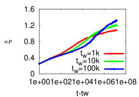
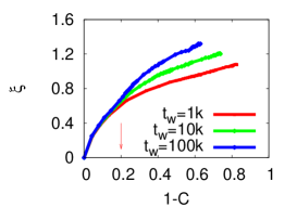
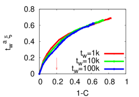
Even though the numerically accessible times are sufficiently long so as to see the separation of time-scales in the relaxation of the global correlation, the correlation length is still very short. In numerical simulations $\xi$ reaches of the order of 4 lattice spacings or inter-particle distances in the spin-glass problem or soft sphere and Lennard-Jones system, respectively. $\xi$ just increases by, say, a factor $4$ when the waiting-time is increased by nearly 4 orders of magnitude. The expected limit $\xi(t,t_{w})\to\infty$ is thus far from being attained.

As we already mentioned in the introduction to this Section, the growing length scale is consistent with the development of time-reparametrization invariance, but it is also consistent with other mechanisms. Hence, it alone cannot be used to argue unambiguously in favor of the symmetry-based approach. For example, theories based on the mode-coupling approach or random first order scenario [33] and its refinement including the effect of entropic droplets [34], dynamical criticality controlled by a zero-temperature critical point [35] and frustration limited domains [36] are used to justify the growth of a dynamic length-scale, at least in the super-cooled liquid. Hence, the existence of a growing length scale belongs to the first class of predictions we mentioned in the introduction to this section.

Finally, let us note that the fluctuations in the susceptibility, or in multi-time correlations, see eq. (41), and associated susceptibilities, can be used to derive other correlation lengths. It would be interesting to check whether all these behave in the same manner.

3.2 Scaling of the pdf of local two-time functions

The most direct way of testing the mere existence of local fluctuations is to measure the probability distribution function (pdf) of local coarse-grained correlators, $C(\vec{r};t,t_{w})$, and linear susceptibilities, $\chi(\vec{r};t,t_{w})$, at different pairs of times, $t$ and $t_{w}$. In such a measurement one is forced to use finite coarse-graining lengths. $\ell$ then becomes a parameters that has to be taken into account in the scaling analysis of the results.

In Ref. [9] we showed that, quite generally, the pdf of local coarse-grained correlators can be scaled onto universal curves as long as the global correlation, $C(t,t_{w})$, is the same, and the ratio of the coarse graining length over the dynamical correlation length, $\ell/\xi(t,t_{w})$, is held fixed (see [31] for a similar discussion applied to the super-cooled liquid). Such scaling can be easily understood as follows. At fixed temperature the pdf $\rho[C_{r};t,t_{w},\ell,L]$ depends on four parameters: two times, $t$ and $t_{w}$, and two lengths, the coarse-graining length, $\ell$, and the size of the system, $L$. As in the aging regime $C(t,t_{w})$ is a monotonic function of the two times and $\xi(t,t_{w})\sim t_{w}^{a}g(C)$, one can trade the two times by $C$ and $\xi$ in complete generality. The next step is a scaling assumption: that in the long times limit the pdfs depend on the coarse graining length $\ell$, the total size $L$ and the scale $\xi$ only through the ratios $\ell/\xi$ and $\xi/L$. This last step, we should stress, is really a scaling assumption, and not a trivial requirement from dimensional analysis. The lengths $\ell$, $L$ and $\xi$ are already dimensionless as they are measured in units of the lattice spacing. The end result from the rewriting of the parameters in terms of the global correlation and the scaling hypothesis is that the pdfs characterizing the heterogeneous constant temperature aging of the system can be written as

$$\rho[C_{r};C(t,t_{w}),\ell/\xi(t,t_{w}),\xi(t,t_{w})/L]\;.$$ (33)

In Fig. 4 we show the scaling of the distribution of local coarse-grained correlations in the $3d$ ea model and the effect of the scaling variable $\ell/\xi$ (the size of the system, $L$, is sufficiently large so that $\xi/L$ vanishes in practice).

Figure 4: pdf of local coarse-grained correlations $C_{r}$ at different times $t$ and $t_{w}$ in the $3d$ Edwards-Anderson model with $L=100$ at $T=0.6<T_{c}$. The waiting-times are given in the key and the global correlation is fixed to $C=0.4<q_{ea}$. (a) The coarse-graining boxes have linear size $\ell=9$ in all cases. The curves do not collapse, a slow drift with increasing $t_{w}$ is clear in the figure. (b) Variable coarse-graining length $\ell$ chosen so as to held $\ell/\xi$ approximately constant. The collapse improves considerably with respect to panel (a). These results are taken from [9].

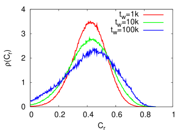
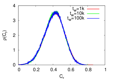
It is noteworthy that a reasonable scaling with the global correlation held fixed and not taking into account the effect of the second scaling variable has been already achieved, approximately, in the Edwards-Anderson model [5, 6], as well as in the kinetically constrained models studied in [7] and Lennard-Jones systems [32]. This is justified by the fact that $\xi$ varies very slowly with $t_{w}$. However, it is clear that at long though finite times one has to hold the ratio $\ell/\xi$ constant to obtain a full collapse in all cases.

The scaling variable $\ell/\xi$ allows one to study the change in the functional form of the pdfs upon modifying the coarse-graining volume. Indeed, the pdfs should crossover from a non-trivial form to a simple Gaussian when $\ell$ goes through the value $\xi$. In summary, for finite $\xi$ one identifies three $\ell$-dependent regimes with different functional forms of the pdfs:

• $\ell\ll\xi$. For finite $\xi$ this means $\ell$ of the order of the lattice spacing, $\ell\sim a$. In this case the pdfs do not have any particular structure.

• $\ell\sim\xi$. For finite but large $\xi$ this case is non-trivial and indeed the one that is accessed with numerical simulations and experiments. One finds that the statistics is non-Gaussian for all $C$. The skewness decreases from zero at $C=1$ to reach a minimum and then increase again at small values of $C$. As regards the functional form, one finds that a Gumbel-like functional form, characterized by a real parameter that depends on $C$ and $\ell/\xi$ describes the data rather well for, say, $q_{ea}/2\stackrel{{\scriptstyle<}}{{\sim}}C\stackrel{{\scriptstyle<}}{{\sim}}q_{ea}$.

• $\ell\gg\xi$. In this limit one matches the central-limit theorem conditions and the statistics becomes Gaussian for all $C$.

The analysis of the $\ell$-dependent pdfs thus provides an independent way to estimate $\xi$.

3.3 Effective action for local ages

The argument leading to eq. (33) is a scaling hypothesis and it does not rely on time-reparametrization invariance. Indeed, there exist models in which the scaling (34) for the pdf of local coarse-grained correlations is found, e.g. the $O(N)$ model in the large $N$ limit [8], and global time-reparametrization does not apply.

The implications of time-reparametrization invariance appear later, as a prediction for the functional form of the asymptotic limit

$$\rho_{\infty}(C_{r};C)\equiv\lim_{\ell\to\infty}\lim_{\stackrel{{\scriptstyle t,t_{w}\to\infty}}{{C(t,t_{w})=C}}}\lim_{L\to\infty}\;\rho[C_{r};C(t,t_{w}),\ell/\xi(t,t_{w}),\xi(t,t_{w})/L]\;.$$ (34)

In order to study the functional form that $\rho_{\infty}$ can take let us now use the symmetry argument to analyse the statistics of the fluctuations of the local correlations. So far we have not yet determined how much the $h(\vec{r},t)$ vary in space and time. To this end we need to derive an effective action for these functions that will tell us how costly it is to deviate from the average clock ${\cal R}(t)$. Ideally, one would like to derive this action from the microscopic one. This should be possible in quasi mean-field models such as the $p$-spin model with Kac long (but finite) range interactions [37]. For the moment we have just proposed the simplest action that serves our purposes in the ideal limit in which the zero mode is fully developed $\xi\to\infty$ and the local quantities are measured in the infinite coarse-graining volume limit with $\ell/\xi\to 0$ [7]. Otherwise the parameter $\ell$ should be taken into account.

To start with we worked with the more convenient transformed variable $h(\vec{r},t)\equiv e^{-\varphi(\vec{r},t)}$ that implies

$$C_{ag}(r;t,t_{w})\approx q_{ea}\;f_{\sc c}\left(\frac{h(\vec{r},t)}{h(\vec{r},t_{w})}\right)=q_{ea}\;f_{\sc c}\left(e^{-\int_{t_{w}}^{t}dt^{\prime}\partial_{t^{\prime}}\;\varphi(\vec{r},t^{\prime})}\right)$$ (35)

and we searched for the simplest action that satisfies the constraints due to the symmetries. These are:

1. The action must be invariant under a global time reparametrization $t\to h(t)$.

2. If our interest is in short-ranged problems, the action must be written using local terms. The action can thus contain products evaluated at a single time and point in space of terms such as $\varphi(\vec{r},t)$, $\partial_{t}\varphi(\vec{r},t)$, $\nabla\varphi(\vec{r},t)$, $\nabla\partial_{t}\varphi(\vec{r},t)$, and similar derivatives.

3. The scaling form in eq. (35) is invariant under $\varphi(\vec{r},t)\to\varphi(\vec{r},t)+\Phi(\vec{r})$, with $\Phi(\vec{r})$ independent of time. Thus, the action must also have this symmetry.

4. The action must be positive definite.

These requirements largely restrict the possible actions. The one with the smallest number of spatial derivatives (most relevant terms) is

$${\cal S}[\varphi]=\int d^{d}r\int dt\left[K\;\frac{\left(\nabla\partial_{t}\varphi(\vec{r},t)\right)^{2}}{\partial_{t}\varphi(\vec{r},t)}\right]\;,$$ (36)

with $K$ a stiffness. A term $M\;\partial_{t}\varphi(\vec{r},t)$ is also allowed by symmetry but since its space-time integral is constant we drop it. The action solely depends on the time derivatives $\partial_{t}\varphi(\vec{r},t)$ and it is simple to check that it satisfies all the four constraints enumerated above (the last requirement follows from the fact that $h(\vec{r},t)$ are monotonically increasing functions of time) [7].

Due to the simple form (36) the $\partial_{t}\varphi(\vec{r},t)$ are uncorrelated at any two different times $t_{1}$ and $t_{2}$. Thus the expression $\Delta\varphi_{\vec{r}}|_{t_{w}}^{t}\equiv\int_{t_{w}}^{t}dt^{\prime}\;\partial_{t^{\prime}}\varphi(\vec{r},t^{\prime})$ entering the exponential in the scaling form in eq. (35) is a sum of uncorrelated random variables in time. One can interpret such expression as the displacement of a random walker with position dependent velocities. Alternatively, one can think of the space-dependent differences $\Delta\varphi_{\vec{r}}|_{t_{w}}^{t}$ as the net space-dependent height (labeled by $t$) of a stack of spatially fluctuating layers $dt\,\partial_{t}\varphi(\vec{r},t)$. The action for the fluctuating surfaces of each layer is given by eq. (36).

The statistics of the $\Delta\varphi_{\vec{r}}|_{t_{w}}^{t}$ are completely determined as follows. The action (36) transforms into one of a Gaussian surface after the introduction of a ‘proper’ time $\tau\equiv\ln{\cal R}(t)$, and the change of variables, $\psi^{2}(\vec{r},t)=\partial_{\tau}\varphi(\vec{r},\tau)$. Indeed,

$$C_{ag}(\vec{r};t,t_{w})\approx f_{\sc c}\left(e^{-\int_{\ln{\cal R}(t_{w})}^{\ln{\cal R}(t)}d\tau^{\prime}\;\psi^{2}(\vec{r},\tau^{\prime})}\right)$$ (37)

$${\cal S}[\psi]=K\int d^{d}r\int d\tau^{\prime}\;[\nabla\psi(\vec{r},\tau^{\prime})]^{2}\;.$$ (38)

Due to the Gaussian statistics of the $\psi$, it is simple to show that connected $N$-point correlations of $\Delta\\ varphi_{\vec{r}_{1}}|^{t}_{t_{w}}$ satisfy

$$\langle\Delta\varphi_{r_{1}}|^{t}_{t_{w}}\;\Delta\varphi_{r_{2}}|^{t}_{t_{w}}\cdots\Delta\varphi_{r_{N}}|^{t}_{t_{w}}\rangle_{c}= [\tau(t)-\tau(t_{w})]\;{\cal F}(\vec{r}_{1},\vec{r}_{2},\dots,\vec{r}_{N})\;,$$ (39)

where the function ${\cal F}$ can be obtained from Wick’s theorem, summing over all graphs that visit all sites (connected) with two lines (because of $\psi^{2}$) for each vertex $i$ corresponding to a position $r_{i}$. The reparametrized times appear only in the prefactor $\tau(t)-\tau(t_{w})=\ln[{\cal R}(t)/{\cal R}(t_{w})]$. The probabilistic features of the fluctuations of local correlations $C(\vec{r},t,t_{w})$ depend on times only through ${\cal R}(t)/{\cal R}(t_{w})$, and hence only through the global correlation itself $C(t,t_{w})$. In consequence, the action (38) implies the scaling (34). The fact that the time-dependencies of the statistical properties of the two-time local coarse-grained correlations are fully determined by the global correlation is a very welcome property of action (36) since it was not obvious a priori.

Having the forms in eqs. (37) and (38) allows us to make some quantitative predictions about the form of the pdfs. With some algebraic manipulations one shows the following generic features [7]:

• The distribution is non-Gaussian for all $C$.

• For $C\stackrel{{\scriptstyle<}}{{\sim}}q_{ea}$ the pdf is negatively skewed and once put into normal form it is very close to the distribution of the global equilibrium magnetization in the $2d$ xy model [38]. It can then be approximately described by a generalized Gumbel form with real parameter.

• In the opposite limit $C\stackrel{{\scriptstyle>}}{{\sim}}0$ the pdf is positively skewed and it does not take any recognizable form.

If one is interested in testing the action further one can simply use eq. (38) to generate, numerically, the $\psi(\vec{r},t)$, construct the $C(\vec{r},t,t_{w})$ from these functions, and then compare the pdfs thus obtained to the ones measured, say, in a numerical simulation of a given problem. Note that the scaling function $f_{c}$ also plays a role in the functional form of the pdf of local correlations. The same argument applies to the susceptibilities.

The local coarse-grained correlations are, by construction, sums of correlated random variables (unless $\ell\gg\xi$). With numerical simulations of the $3d$ ea model [9] and kinetically facilitated lattice gases [7] we found that the pdfs of correlations coarse-grained over finite lengths $\ell$ have a functional form that resembles a generalized Gumbel distribution characterized by a continuous parameter that depends on $\ell/\xi$ and the value of the global correlation, $C$, when $C\stackrel{{\scriptstyle<}}{{\sim}}q_{ea}$ (see also [38]). This fact is consistent with the discussion above and also with the observation of Bertin and Clusel that Gumbel-like pdfs with real parameter characterize the statistics of sums of random variables with particular correlations between the elements [39]. The fact that we obtain Gumbel-like distributions then means that the correlations between the terms in the sum are of the form needed to get this type of pdf.

In short, the time-reparametrization scenario predicts, in its simplest setting, that eqs. (37) and (38) fully characterise the fluctuation of the local correlations in the large times and coarse-graining volume limits.

3.4 Two-time scaling of local functions

As we argued in Sect. 2.4, the global time-reparametrization invariance suggests that in the ideal asymptotic limit the slow part of the coarse-grained local correlations and susceptibilities should scale as in eq. (26) in the ideal limit $a\ll\ell\ll\xi$. In practice the ideal limit is not reached and one is forced to work with finite correlation lengths and thus finite coarse-graining lengths too. The finite $\ell$ will then play a role and has to be taken into account. We now present some tests of eq. (26) that are based on the parametric representation of the dynamics explained in Sect. 2 and take into account the finite value of $\ell$.

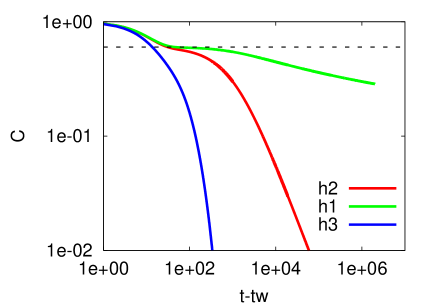
Let us then imagine that we compute three local coarse-grained two-time correlations, $C_{\vec{r}}$, at three space points $\vec{r}_{1}$, $\vec{r}_{2}$ and $\vec{r}_{3}$, using a given coarse-graining length, $a\ll\ell$, and that we obtain functional forms that are characterized by eq. (26) with, say, $h(\vec{r}_{1},t)=\ln\left(t/t_{0}\right)$, $h(\vec{r}_{2},t)=t/t_{0}$, and $h(\vec{r}_{3},t)=e^{\ln^{2}\left(t/t_{0}\right)}$, in the aging regime. In Fig. 5 we sketch the decay of these correlations for the same $t_{w}$ as a function of time-delay. The plateau is at the same height since $q_{ea}$ as well as the the full stationary decay are not expected to fluctuate. The external function $f_{c}$ is the same in all curves. It is clear that the decay of the three correlations follows a different pace, the one at $\vec{r}_{3}$ is the fastest while the relaxation at $\vec{r}_{2}$ is the slowest.

                          

Figure 5: Left: sketch of the decay of the correlation with the same stationary decay to $q_{ea}$ – shown with a horizontal dashed line – and three choices of the scaling function $h(r_{1},t)=\ln(t/t_{0})$, $h(r_{2},t)=t/t_{0}$, and $h(r_{3},t)=e^{\ln^{a}(t/t_{0})}$. The waiting-time is the same in all curves. Right: the relation between the integrated linear response against the correlation. With a solid line, the parametric plot for fixed and long $t_{w}$, using $t$ as a parameter that increases from $t_{w}$ at $C=1$ to $\infty$ at $C=0$. With symbols, the three pairs $(C_{j}(t,t_{w}),\chi_{j}(t,t_{w}))$ for the same $t_{w}$, a fixed value of $t$ and $h_{j}(t)$ as in the left panel.

Figure 6: The triangular relation in the $3d$ ea model. Upper left panel: the thick (black) line represents the global $C(t_{1},t_{2})$ against $C(t_{2},t_{3})$ using $t_{2}$ as a parameter varying between $t_{3}=5\times 10^{4}$ MCs and $t_{1}=9\times 10^{6}$ MCs, $C(t_{1},t_{3})\sim 0.35$ and $q_{ea}\sim 0.8$. The curved part is well represented by the hyperbolic form $C(t_{1},t_{2})\sim q_{ea}C(t_{1},t_{3})/C(t_{2},t_{3})\sim 0.79\times 0.35/C(t_{2},t_{3})$ that corresponds to $f_{c}(x)\sim x^{-b}$. With different points joined with thin lines we show the triangular relations between the local coarse-grained correlations on five randomly chosen sites on the lattice ($\ell=30$). Upper right panel and lower left and right panels: $2d$ projection of the joint probability density of $C(r;t_{1},t_{2})\sqrt{C(t_{1},t_{3})/C(r;t_{1},t_{3})}$ and $C(r;t_{2},t_{3})\sqrt{C(t_{1},t_{3})/C(r;t_{1},t_{3})}$ at fixed three values of the intermediate time, $t_{2}=1.5\times 10^{5}$ MCs, $8\times 10^{5}$ MCs and $5\times 10^{6}$ MCs, respectively and $\ell=10$. The global $C(t_{1},t_{2})$ against $C(t_{2},t_{3})$ using $t_{2}$ as a parameter is shown with a thick green line. The green points indicate the location of $C(t_{1},t_{2})$ and $C(t_{2},t_{3})$ for the chosen $t_{2}$’s. Each point in the scatter plot corresponds to a site, $r$. The lines indicated the boundary surrounding 25%, 50% and 75% of the probability density. The cloud extends mostly along the global relation as predicted by time-reparametrization invariance. These results are taken from [9].

The simplest way to put the proposal (26) to the test is to analyze the implications of eq. (26) on local triangular relations. In Sect. 2 we showed that two-time functions with a separation of time-scales as in eq. (8) and an aging scaling as in eq. (13) are related in a parametric way in which times disappear, see the sketch in Fig. 2-left. Equation (26) implies that the local (fluctuating) two-time functions should verify the same relation

$$C_{ag}(\vec{r};t_{1},t_{3})=q_{ea}\;f_{c}\left\{f^{-1}_{c}[C_{ag}(\vec{r};t_{1},t_{2})/q_{ea}]\;f^{-1}_{c}[C_{ag}(\vec{r};t_{2},t_{3})/q_{ea}]\right\}\;.$$ (40)

This is a result of the fact that time-reparametrization invariance restricts the fluctuations to appear only in the local functions $h(\vec{r},t)$ while the function $f_{c}$ is locked to be the global one everywhere in the sample.

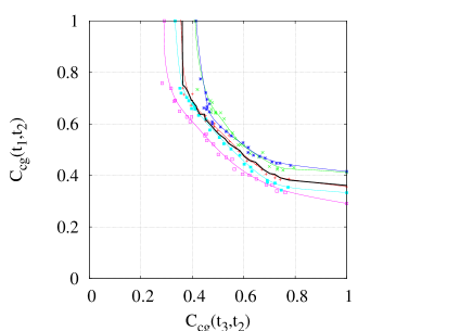
A pictorial inspection of this relation should take into account the fact that while the stationary decay is not expected to fluctuate, the full aging relaxation and, in particular, the minimal value of the local two-time functions, $C(\vec{r};t_{1},t_{3})$, are indeed fluctuating quantities. The parametric construction on different spatial regions should yield ‘parallel translated’ curves with respect to the global one, as displayed in Fig. 2-left. Fluctuations in the function $f_{c}$ would yield different functional forms in the curved part of the parametric construction. A more quantitative analysis can be done by using the knowledge of $f_{c}$ that can be extracted from the global correlation decay. Indeed, if $f_{c}$ is known, the parametric plot $f_{c}^{-1}(C_{\vec{r}12}/q_{ea})/\sqrt{f_{c}^{-1}(C_{\vec{r}13}/q_{ea})}$ against $f_{c}^{-1}(C_{\vec{r}23}/q_{ea})/\sqrt{f_{c}^{-1}(C_{\vec{r}13}/q_{ea})}$ should yield a master curve identical to the global one with different sites just being advanced or retarded with respect to the global value. This is another way of stating that the sample ages in a heterogeneous manner, with some regions being younger (other older) than the global average. (For simplicity we used a chort-hand notation, $C_{{\vec{r}}\mu\nu}=C(\vec{r};t_{\mu},t_{\nu})$ with $\mu,\nu=1,2,3$.) If the time-reparametrization mode is indeed flat the local values should lie all along this master curve in the aging regime.

The conclusions drawn above apply in the strict $a\ll\ell\ll\xi$ limit. In simulations and experiments $\xi$ is finite and even rather short. Thus, $\ell$ is forced to also be a rather small parameter, in which case ‘finite size’ fluctuations in $f_{c}$ are also expected to exist. The claim is that the latter should scale down to zero faster (in $\ell$) than the fluctuations that are related to the zero mode.

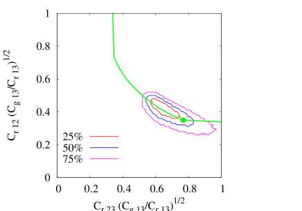
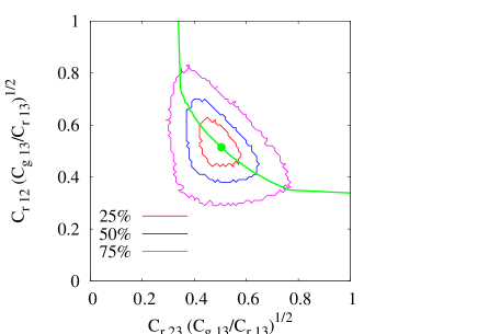
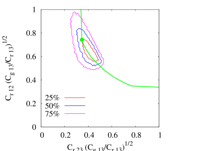
We have tested these claims in the non-equilibrium dynamics of the $3d$ ea spin-glass [9]. The results are shown in Fig. 6. In the upper left panel we show the global triangular relation (thick black line) as well as the local one on four chosen sites. The separation of time-scales is clear in the plot. The aging part is rather well described by $f_{c}(x)\sim x^{-b}$ and the local curves are quite parallel indeed. In the remaining panels in Fig. 6 we show the $2d$projection of the joint probability density of the site fluctuations in the local coarse-grained correlations at different chosen times $t_{2}$, $t_{2}=1.5\times 10^{5}$ MCs (upper right), $t_{2}=8\times 10^{5}$ MCs (lower left), and $t_{2}=5\times 10^{6}$ MCs (lower right). Taking advantage of the fact that $f_{c}(x)\sim x^{-b}$ we use a very convenient normalization in which we multiply the horizontal and vertical axes by $[C_{13}/C_{{\vec{r}}13}]^{1/2}$. Global time-reparametrization invariance, expressed in eq. (40), implies that the data points should spread along the global curve indicated with a thick green line in the figure. Some sites could be advanced, others retarded, with respect to the global value – shown with a point on the green curve – but all should lie mainly on the same master curve. This is indeed quite well reproduced by the simulation data in the three cases, $C(t_{1},t_{2})$ close to $C(t_{1},t_{3})$ (upper right panel), $C(t_{1},t_{2})$ close to $q_{ea}$ (lower right panel), and $C(t_{1},t_{2})$ far from both (lower left panel). Most of the data points tend to follow the master curve though some fall away from it. The reason for this is that eq. (40) should be strictly satisfied only in the very large coarse-graining volume limit ($\ell\gg a$) with $\ell/\xi\ll 1$ while we are here using $\ell=10a\sim\xi$, see the discussion in Sect. 3.1.

The triangular relation can be used to test the fluctuations of the local susceptibilities too. Indeed, if the separation of time scales (8) and the scaling (13) apply to the global susceptibility, the local ones, after the convenient normalization by the maximum value, should follow another master curve, identical to the global one. Note that time-reparametrization invariance as we discuss it here implies that both local correlations and susceptibilities should be fluctuating quantities.

Finally, notice that, in contrast to the growing correlation length scale, there is no blatantly obvious explanation of these triangular relations within other theoretical scenarios. These relations are perhaps the most direct consequence of the time reparametrization symmetry arguments, and so this prediction falls within the second class we discussed in the introduction to this section.

3.5 Multi-time scaling

In general muti-time correlations are non-trivially related to two-time ones. One can take as an example a generic coarse-grained connected four-time correlation. If this function is monotonic with respect to all times, and the two-point correlations scale as in (13) for all pairs $(t_{\mu},t_{\nu})$ with $\mu,\nu=1,2,3,4$, the four-time correlation should behave as

$$C(\vec{r};t_{1},t_{2},t_{3},t_{4})=g\left(\frac{h(\vec{r},t_{1})}{h(\vec{r},t_{2})},\frac{h(\vec{r},t_{2})}{h(\vec{r},t_{3})},\frac{h(\vec{r},t_{3})}{h(\vec{r},t_{4})}\right)$$ (41)

with the same external function $g$ for all $r$, in the asymptotic limit in which all times are widely separated and the corresponding two-time correlations fall below $q_{ea}$. Parametric constructions could be envisaged to test this relation.

3.6 Local fluctuation-dissipation relation

The asymptotic relation between the global correlation and susceptibility

$$\lim_{t_{w}\to\infty,C(t,t_{w})=C}\chi(t,t_{w})=\hat{\chi}(C)$$ (42)

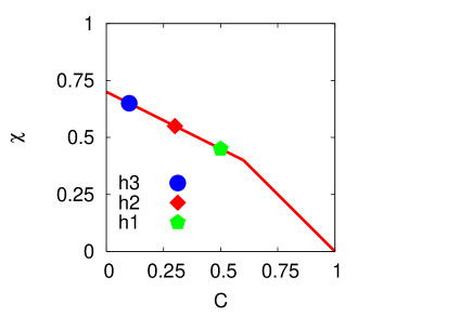
was first obtained in mean-field disordered models [12, 13] and later observed in simulations of many realistic systems (spins and particles in interaction on finite dimensional spaces). $-(d_{C}\hat{\chi}(C))^{-1}$ defines an effective temperature [14]. In the aging regime, that is to say for $C<q_{ea}$, three behaviours have been observed in mean-field systems: in structural glass models $\hat{\chi}(C)$ is linear in $C$ (solid line in the right-panel in Fig. 5); in spin-glass models $\hat{\chi}(C)$ is a non-linear function of $C$; in coarsening systems $\hat{\chi}(C)$ is a constant equal to $(1-q_{ea})/T$.

The scaling in eq. (26) implies that the parametric construction ‘local susceptibility against local correlation’ should fall on the master curve for the global quantities but can be advanced or retarded with respect to the global value; again in the theoretical limit $a\ll\ell\ll\xi$. This behaviour is sketched in Fig. 5-right for the three sites whose correlations are displayed in the left panel. The restricted relation between local susceptibility and local correlation in eq. (26) arise from the fact that the fluctuations are due to local reparametrizations alone and not to changes in the external functions $f_{c}$ and $f_{\chi}$ (much as in transverse vs. longitudinal fluctuations in a non-linear $\sigma$-model).

An important property of the interpretation of the fluctuation dissipation relation in terms of effective temperatures is that one expects all observables evolving in the same time-scale to equilibrate and hence have the same value of the effective temperature [14] in an asymptotic regime with slow dynamics and small entropy production. Within the time-reparametrization invariance approach the local effective temperature, defined from the slope of the $\hat{\chi}(C)$ plot, is automatically the same in the whole sample within a correlation scale, just because the functions $f_{c}$ and $f_{\chi}$ do not fluctuate.

In Fig. 7 we show the joint pdf of local correlations and susceptibilities of the $3d$ ea spin-glass in its glassy phase; the accord with the analytic prediction is very satisfactory [5, 6] with the additional spreading away from the master curve ascribed to the fact that $\ell$ is finite and not very different from $\xi$.

Figure 7: (a) The joint pdf $\rho(C_{r},\chi_{r})$ at two times $(t_{w},t)$ such that the global correlation is $C(t,t_{w})=0.7<q_{\sc ea}$ in the $3d$ ea model. (b) Projection of three contour levels. The crosses are the parametric construction $\hat{\chi}(C)$ for several values of the total time $t$ larger than $t_{w}$. The dotted straight line is fdt at the working temperature $T$. These results are taken from [6].

3.7 Infinite susceptibilities

Zero modes are intimately related to infinite susceptibilities. Indeed, systems with continuous symmetries are sensitive to arbitrarily weak perturbations. In the present context the approximate global time-reparametrization invariance implies that one can easily change the ‘clock’ ${\cal R}(t)$ characterizing the scaling of the global correlation and linear response by applying infinitely weak perturbations that couple to the zero mode. An illustration of this property is the fact that the aging relaxation dynamics of glassy systems is rendered stationary by a weak perturbing force that does not derive from a potential while the $\hat{\chi}(C)$ relation in the slow regime is not modified [40]. One could envisage more refined tests such as applying a perturbation that imposes different scalings on two macroscopic borders of the system and see how the time-reparametrization wave develops in the bulk.

3.8 Conclusions

In conclusion, the global time-reparametrization invariance scenario gives a mechanism for the divergence of the correlation length $\xi$ though others have also been proposed in the literature. There are a number of predictions, as the parametric relations between local coarse-grained correlations measured at different times and the local fluctuation-dissipation relations that, to our knowledge, are not explained by other scenarios. As regards to the easier to measure pdfs of local correlations the framework is not only consistent with the scaling (34) – that also arises from simple scaling assumptions – but it also justifies the non-Gaussian and Gumbel-like functional form of the pdfs that follows from the proposed effective action for local ‘ages’. Moreover, systems with global time-reparametrization invariance should have as important fluctuations in the local susceptibilities as in the local coarse-grained responses.

4 Discussion

We presented a summary of studies of dynamical fluctuations in glassy systems that are based on the idea that, in the long time regime, a global time-reparametrization invariance emerges in the effective action describing the aging dynamics. We discussed how this symmetry concretely appears in mean-field spin models, and how it can be shown to emerge at the level of the action for short-ranged spin glass models with quenched disorder. Two assumptions are used to prove the global time-reparametrization of the action for the short-range spin glass model i) causality and unitarity, and ii) a separation of time scales between a fast (or stationary) and a slow (or aging) relaxation, where in the latter time translation invariance is broken.

That the dynamical action is symmetric under uniform, i.e., spatially independent reparametrizations of time variables ($t\to h(t)$) suggests that the dynamic fluctuations that cost little action should be describable in terms of position dependent, long wavelength, reparametrizations of the form $t\to h({\vec{r}},t)$. These should be the Goldstone modes associated with breaking time-reparametrization invariance symmetry.

We presented predictions of this theoretical framework and tests that we performed in the $3d$ Edwards-Anderson model to falsify these predictions. Among the consequences of our theoretical framework are those listed in Sect. 3. Some of them find an explanation within other theories as well; others are particularly related to the time reparametrization invariance scenario. For example, a correlation length that grows in time is associated with the asymptotic approach to the long-time regime in which the symmetry is fully developped, and the long wavelength modes eventually become massless. The existence of a growing length is also predicted by other models. The functional form of the triangular relations relating local two-time correlations between three different times is, instead, particular to our framework.

In this review we showed tests of the predictions of the global time-reparametrization invariance scenario performed on a finite dimensional spin-glass model [4]-[9]. In the past we also studied the dynamics of kinetically facilitated models, without quenched disorder, along the same lines [7]. We believe that, if aging dynamics is a universal property of glassy systems, then these ideas should also apply to interacting particle systems without quenched disorder. The rationale is that the two assumptions leading to the global time-reparametrization invariance of the dynamical action, namely causality and unitarity, and a separation of time scales, should also hold for other glassy systems. The former assumption we can take as a fact. The second is, in a way, the assumption that a glassy phase exists, even though we say nothing as of why it does. As we stated in the introduction, we do not aim at the question why glasses?, but instead we focus on the possible universal dynamical properties once the glassy state is presented by nature. Some of the consequences of the symmetry have already been tested numerically in Lennard-Jones systems [29, 32] but there is still much room for more detailed studies, including the analysis of local triangular relation between correlation and susceptibilities and tests of their joint behaviour.

We thus propose that the asymptotic global time-reparametrization invariance, and the associated low action long wavelength local reparametrizations, constitute the mechanism by which dynamic fluctuations, that is to say heterogeneities, are generated in the glassy state. Moreover, this mechanism may also apply, in an approximate form, to the super-cooled liquid regime. It should just be an approximation because in super-cooled liquids the symmetry is not fully developed and there is then a cut-off setting the limit of the spatial and temporal extent of the heterogeneities, in sharp constrast to the low temperature glassy regime in which the symmetry is realized asymptotically and fluctuations of all sizes exist. The growth and divergence of the (two-time) dynamic correlation length defined from the study of the space correlation of the two-time order parameter is a manifestation of the growth and divergence of these fluctuations in the glassy state; in contrast, such growth is interrupted in the super-cooled liquid.

To better understand the distiction between the glassy state with its asymptotic symmetry and the super-cooled state without the fully developing symmetry, consider the phenomenology of dynamic fluctuations as a function of temperature. Dynamic heterogeneities in the super-cooled liquid phase have been identified numerically and experimentally [52]. These are in a number of ways more important than what is observed in a simple liquid or a solid. In the super-cooled liquid phase while the full relaxation is stationary, there is still a time-scale separation with the correlations decaying as a function of time-difference first rapidly to a temperature-independent plateau and then slowly towards zero. The latter is the structural or $\alpha$-relaxation. The $\alpha$ relaxation time, $t_{\alpha}$, is finite in the super-cooled liquid regime and it increases upon decreasing temperature. The global parametrization chosen by the symmetry breaking terms in the slow regime is ${\cal R}(t)\propto e^{-t/t_{\alpha}}$ and $C(t,t_{w})=q_{ea}f_{c}(e^{-(t-t_{w})/t_{\alpha}})$ in this case.

The mode-coupling approach to super-cooled liquids is based on approximate dynamic equations for the relevant correlators of realistic systems that are very similar to the $p$-spin Schwinger-Dyson equations in the high temperature phase [16, 18]. In these equations the correlators are already expressed as functions of the time-difference, $\tau\equiv t-t_{w}$. Close to the critical temperature the separation of time-scales develops in the mode-coupling equations. The approximate analysis of the $\alpha$ relaxation predicted by these equations also relies on dropping the $\tau$ derivatives and approximating the integrals by assuming a sharp time-scale separation. The remaining asymptotic (large $\tau$) equations are invariant under reparametrizations of $\tau$.

We then expect the local coarse-grained correlations and integrated linear responses in the super-cooled liquid to be, to a first approximation, stationary (after a sufficiently long waiting-time that goes beyond the equilibration time) but with different finite structural relaxation times, fluctuating about the value that characterizes the decay of the global correlations. This is consistent with the experimental observation that dynamic heterogeneities in supercooled liquids seem to have a lifetime of the order of the relaxation time. Deviations from stationarity are not completely excluded for finite $\ell$ but they should be less important than in the aging low-temperature regime.

There is, however, an important difference with respect to the aging regime, in which the equilibration time diverges and local relaxation times or, better stated, local ages can fluctuate without limit when $t_{w}\to\infty$. At high temperatures one does not expect to find heterogeneities with arbitrary long relaxation time. Furthermore, heterogeneities have a finite spatial extent and one can then suppress them by using sufficiently large coarse-graining volumes. The correlation length is stationary, $\xi(\tau)$, and it saturates in the limit of long-time differences, $\tau\to\infty$. The saturation value, though, increases for decreasing temperature. From a theoretical point of view, this picture is, in a sense, similar to the one that describes the equilibrium paramagnetic phase in the $O(N)$ model, just above the ordering transition temperature.

When lowering the temperature the size and life-time of the heterogeneities increases. A $p$-spin or mode-coupling approach predicts that their typical size and thus $\lim_{\tau\to\infty}\xi(\tau)$ diverge at the mode coupling transition temperature [33]. In real systems the divergence at $T_{c}$ is rendered smooth and $\xi$ does not strictly diverge asymptotically.

At still lower temperatures the bulk quantities age and we expect then to observe heterogeneous aging dynamics of the kind described in this review, with a two-time dependent correlation length for the local fluctuations. The heterogeneities age as well, in a ‘dynamic’ way. By this we mean that if a region looks older than another one when observed on a given time-window, it can reverse its status and look younger than the same other region when observed on a different time-window.

The infinite susceptibility with respect to perturbations that couple to the zero mode are illustrated by the fact that the clock of the bulk quantities that is selected dynamically is very easy to modify with external perturbations. A small force that does not derive from a potential and is applied on every spin in the model renders an aging $p$ spin model stationary [40] while the model maintains a separation of time-scales in which the fast scale follows the temperature of the bath, $T$, while the slow scale is controlled by an an effective temperature, $T_{\sc eff}>T$. In this case, the aging system selects a time-reparametrization ${\cal R}(t)=t$ while in the perturbed model ${\cal R}(t)=e^{-t/t_{\alpha}}$. Similarly, the aging of a Lennard-Jones mixture is stopped by an homogeneous shear [41]. A different way to modify the time-reparametrization that characterizes the decay of the correlations is by using complex thermal baths [42].

The picture that we have described applies to long times but not as long as to enter the activated regime that we still do not know how to characterize theoretically, not even at the bulk level. This regime corresponds to times that scale with the system size. The success of mean-field models, or the mode-coupling approach, in describing the bulk dynamics of glassy systems, at least not to close to the crossover glass temperature and at a qualitative level, allows us to claim that these extremely long times scales are unrealistic if not too close to the glass transition $T_{g}$ even as far as dynamic fluctuations are concerned.

The ideas discussed in this paper should not only apply to systems that relax in a non-equilibrium manner as glasses but also to systems with slow dynamics and a separation of time-scales that are kept out of equilibrium with a (weak) external forcing. Recently, there has been much interest in the appearance of shear localization, in the form of shear bands, in the rheology of complex fluids. Along the lines here described it would be very interesting to analyze the fluctuations in the local reparametrizations in the fluidized shear band and the ‘jammed’ glassy band.

The analytic treatment of mean-field quantum glassy systems follows similar steps to the ones presented here. The Schwinger-Keldysh approach replaces the Martin-Siggia-Rose one but these formalisms are very similar indeed. The analytic solution to the dynamic equations in the limit in which the coupling to the environment is weak also uses the fact that the dynamics in the aging regime is very slow. The approximate equations then become time-reparametrization invariant. One can then expect that similar dynamic fluctuations arise in glassy problems in which quantum fluctuations are important. Moreover the proof of global time-reparametrization invariance for spin-glasses has been presented directly in the quantum formalism. Novel experimental techniques may be apt to study dynamic heterogeneities in glasses when quantum fluctuations are important.

We expect to find similar fluctuations using finite size systems and examining the behaviour of the mesoscopic run-to-run fluctuations of the global correlations. These may be easier to measure experimentally using mesoscopic systems.

Importantly enough, global time reparametrization invariance does not develop in all models with slow and aging correlation functions. The O(N) ferromagnetic model in the large $N$ limit is a case in which global time-reparametrization invariance is reduced to just scale invariance [8].

Last, but not least, the approach based on reparametrization invariance suggests that it may be possible to search for universality in glassiness. A Ginzburg-Landau theory for phase transitions captures universal properties that are independent of the details of the material. It is symmetry that defines the universality classes. For example, one requires rotational invariance of the Ginzburg-Landau action when describing ferromagnets. Time reparametrization invariance may be the underlying symmetry that must be satisfied by the Ginzburg-Landau action of all glasses. What would determine if a system is glassy or not? We are tempted to say the answer is if the symmetry is generated or not at long times. Knowing how to describe the universal behavior may tell us all the common properties of glasses, but surely it will not allow us to make non-universal predictions, such as what is the glass transition temperature for a certain material, or whether the material displays glassy behavior at all. This quest for universality is a very interesting theoretical scenario that needs to be confronted.

We have tried to state as clearly as possible the implications of our proposal. The full project is not yet complete since several questions about its limitations remain open. A number of issues should be addressed are:

(i) From a phenomenological point of view, to perform strong tests of the global time-reparametrization invariance scenario in molecular dynamic simulations [28, 44, 45] of realistic glassy systems and experiments [46]-[51]. More precisely, the triangular relations between local coarse-grained correlations and the local fluctuation dissipation relations should be analysed to give support or else falsify this conjecture.

(ii) From an analytic point of view, to derive the effective action for local reparametrizations for glassy models with and without quenched disorder. We are currently working on this project in collaboration with S. Franz. One idea is to study the $p$ spin disordered model with Kac long-range interaction. ANothe one is to study the symmetries of the dynamic action associated with the Dean-Kawasaki equation for the evolution of the density of a system of particles in interaction.

(iv) From a mixed analytic and numerical point of view to analyse fluctuations in models with global aging dynamics of different type. To this end, one can study dynamic fluctuations in simple coarsening systems in finite dimensions. In these cases the morphology of domains can be characterized in great detail [43]. We could, in principle, understand the fluctuations in the local correlations and linear responses from a microscopic point of view. Whether these are similar or different to the ones in other glassy problems is still to be established and the outcome of this study could clarify the relevance of the value of the effective temperature in determining the characteristics of the dynamic fluctuations.

(v) In the same line as the above, the analysis of fluctuations of elastic lines in the presence of impurities could help us understanding the coarsening phenomenon but also the role of diffusion that superimposes in these cases to the aging dynamics [15].

These are just a few questions posed by this proposal that are still not answered.

Acknowledgments

We thank our collaborators J. J. Arenzon, C. Aron, A. J. Bray, S. Bustingorry, H. E. Castillo, P. Charbonneau, D. Domínguez, J. L. Iguain, L. D. C. Jaubert, M. P. Kennett, M. Picco, D. R. Reichman, M. Sellitto, A. Sicilia and H. Yoshino.

We also wish to especially thank L. Berthier, G. Biroli, J-P Bouchaud, D. S. Dean, G. Fabricius, T. Grigera, E. Fradkin, S. Franz, J. Kurchan, H. Makse, D. Stariolo and L. Valluzzi for very helpful discussions. We acknowledge financial support from NSF-CNRS INT-0128922, NSF DMR-0305482, DMR 0403997 and PICS 3172. LFC is a member of Institut Universitaire de France. LFC thanks the Newton Institute at the University of Cambridge, ICTP at Trieste, and Universidad Nacional de Mar del Plata, Argentina, CC the LPTHE at Jussieu, Paris, France, and LFC and CC the Aspen Center for Physics for hospitality where part of this work has been carried out.

References

- [1] M. D. Ediger, C. A. Angell, and S. R. Nagel; J. Phys. Chem. 100, 13 200 (1996). Glassy Materials and disordered solids, K. Binder and W. Kob (World Scientific, 2005).
- [2] P. W. Anderson, Concepts in solids, (World Scientific, 1997).
- [3] Several reviews and book summarize the aging properties of different types of glasses. Aging in polymer glasses is described in L. C. D. Struik, Physical aging in amorphous polymers and other materials (Elsevier, Houston, 1978). Aging in spin-glasses is reviewed in E. Vincent et al, Slow dynamics and aging in spin-glasses, cond-mat/9607224. Aging in soft glassy materials is summarized in L. Cipelletti and L. Ramos, J. Phys. C 17, R253 (2005). or Viasnoff and Lequeux. Aging in orientational glasses in F. Alberici-Kious, J-P Bouchaud, L. F. Cugliandolo, P. Doussineau and A. Levelut, Phys. Rev. B 62, 14766 (2000)
- [4] C. Chamon, M. P. Kennett, H. E. Castillo, and L. F. Cugliandolo Phys. Rev. Lett. 89, 217201 (2002).
- [5] H. E. Castillo, C. Chamon, L. F. Cugliandolo, and M. P. Kennett, Phys. Rev. Lett. 88, 237201 (2002).
- [6] H. E. Castillo, C. Chamon, L. F. Cugliandolo, J. L. Iguain, and M. P. Kennett, Phys. Rev. B 68, 134442 (2003).
- [7] C. Chamon, P. Charbonneau, L. F. Cugliandolo, D. R. Reichman, and M. Sellitto, J. of Chem. Phys. 121, 10120 (2004).
- [8] C. Chamon, L. F. Cugliandolo, H. Yoshino, J. Stat. Mech (2006) P01006.
- [9] L. D. C. Jaubert, C. Chamon, L. F. Cugliandolo, and M. Picco, cond-mat/0701116, to appear in JSTAT.
- [10] H. Sompolinsky, Phys. Rev. Lett. 47, 935 (1981).
- [11] S. L. Ginzburg, Zh. Eksp. Teor. Fiz. 90, 754 (1986) [Sov. Phys. JETP 63, 439 (1986)]. L. B. Ioffe, Phys. Rev. B 38, 5181 (1988).
- [12] L. F. Cugliandolo and J. Kurchan, Phys. Rev. Lett. 71, 173 (1993).
- [13] L. F. Cugliandolo and J. Kurchan, J. Phys. A 27, 5749 (1994).
- [14] L. F. Cugliandolo, J. Kurchan, and L. Peliti, Phys. Rev. E 55, 3898 (1997).
- [15] S. Bustingorry, J. L. Iguain, C. Chamon, L. F. Cugliandolo, and D. Domínguez, Europhys. Lett. 76, 856 (2006).
- [16] T. R. Kirkpatrick and D. Thirumalai, Phys. Rev. Lett. 58, 2091 (1987); Phys. Rev. B 36, 5388 (1987). T. R. Kirkpatrick and P. Wolynes, Phys. Rev. B 36, 8552 (1987).
- [17] C. Chamon and M. P. Kennett, Phys. Rev. Lett. 86, 1622 (2001).
- [18] J-P Bouchaud, L. F. Cugliandolo, J. Kurchan, and M. Mézard, Physica A 226, 243 (1996).
- [19] L. F. Cugliandolo, Lecture notes in Slow Relaxation and non equilibrium dynamics in condensed matter, Les Houches Session 77 July 2002, J-L Barrat, J Dalibard, J Kurchan, M V Feigel’man eds. (Springer-Verlag, 2003); cond-mat/0210312.
- [20] W. Götze and L. Sjögren, Rep. Prog. Phys. 55, 241 (1992). W. Götze, Condensed Matter Physics 1, 873 (1998).
- [21] R. A. Fisher, Ann. Eugenetics, 7, 355 (1937).
- [22] V. Viasnoff and F. Lequeux, Phys. Rev. Lett. 89, 065701 (2002).
- [23] D. S. Dean, J. Phys. A 29, L613 (1996). K. Kawazaki and T. Koga, Physica A 201, 115 (1993).
- [24] L. F. Cugliandolo and D. S. Dean, J. Phys. A 28, 4213 (1996).
- [25] L. F. Cugliandolo and G. S. Lozano, Phys. Rev. Lett. 80, 4979 (1998).
- [26] L. F. Cugliandolo, D. R. Grempel, G. L. Lozano, H. Lozza, and C. A. da Silva Santos, Phys. Rev. B 66, 014444 (2002).
- [27] C. De Dominicis and E. Brézin, Eur. Phys. J. B 30, 71 (2002)
- [28] G. Parisi, J. Phys. Chem. B 103, 4128 (1999).
- [29] A. Parsaeian and H. E. Castillo, cond-mat/0610789.
- [30] see e.g. N. Lačević, F. W. Starr, T. B. Sch/oder, and S. C. Glotzer, J. Chem. Phys. 119, 7372 (2003) and references therein.
- [31] L. Berthier, Phys. Rev. E 69, 020201(R) (2004).
- [32] H. E. Castillo and A. Parsaeian, cond-mat/0610857.
- [33] S. Franz and G. Parisi, J. Phys. I 5, 1401 (1995), Phys. Rev. Lett. 79, 2486 (1997). C. Donati, S. Franz, G. Parisi, and S. C. Glotzer, Phil. Mag. B 79, 1827 (1999). G. Biroli and J-P Bouchaud, Europhys. Lett. 67, 21 (2004). G. Biroli, J-P Bouchaud, K. Miyazaki, and D. R. Reichman, cond-mat/0605733.
- [34] T. R. Kirkpatrick and P. Wolynes, Phys. Rev. B 36, 8552 (1987). T. R. Kirkpatrick, D. Thirumalai and P. G. Wolynes, Phys. Rev. A 40, 1045 (1989). P. G. Wolynes, Jour. Res. NIST 102, 187 (1997). J-P Bouchaud and G. Biroli, J. Chem. Phys. 121, 7347 (2004).
- [35] J. P. Garrahan and D. Chandler, Proc. Natl. Acad. Sci. USA 100, 9710 (2003). S. Whitelam, L. Berthier, and J. P. Garrahan Phys. Rev. Lett. 92, 185705 (2004). A. C. Pan, J. P. Garrahan, and D. Chandler Phys. Rev. E 72, 041106 (2005). R. L. Jack, L. Berthier, and J. P. Garrahan, Phys. Rev. E 72, 016103 (2005). R. L. Jack and J. P. Garrahan, J. Chem. Phys. 123, 164508 (2005),
- [36] G. Tarjus, S. A. Kivelson, Z. Nussinov, and P. Viot, The frustration-based approach of supercooled liquids and the glass transition: a review and critical assessment, cond-mat/0509127 and references therein.
- [37] C. Chamon, L. F. Cugliandolo and S. Franz, in preparation.
- [38] S. Bramwell, P. C. W. Holdsworth and J-F Pinton, Nature 396, 552 (1998).
- [39] E. Bertin and M. Clusel, J. Phys. A 39, 7607 (2006).
- [40] L. F. Cugliandolo, J. Kurchan, P. Le Doussal, and L. Peliti, Phys. Rev. Lett. 78, 350 (1997). L. Berthier, J.-L. Barrat, and J. Kurchan, Phys. Rev. E 61, 5464 (2000).
- [41] L. Berthier and J.-L. Barrat, Phys. Rev. Lett. 89, 095702 (2002); J. Chem. Phys. 116, 6228 (2002).
- [42] L. F. Cugliandolo and J. Kurchan, Physica A 263 242 (1999).
- [43] J. J. Arenzon, A. J. Bray, L. F. Cugliandolo, and A. Sicilia, cond-mat/0608270, to appear in Phys. Rev. Lett.
- [44] L. Valluzzi et al., in preparation.
- [45] K. Vollmayr-Lee, W. Kob, K. Binder, and A. Zippelius, J. Chem. Phys. 116, 5158 (2002).
- [46] L. Buisson, L. Bellon, and S. Ciliberto, cond-mat/0210490, to appear in Proceedings of “III Workshop on Non-Equilibrium Phenomena” (Pisa 2002).
- [47] W. K. Kegel and A. V. Blaaderen, Science 287, 290 (2000).
- [48] K. S. Sinnathamby, H. Oukris, N. E. Israeloff, Phys. Rev. Lett. 95, 67205 (2005). Crider and N. E. Israeloff, Nano Letters 6, 887 (2006).
- [49] L. Cipelletti, H. Bissig, V. Trappe, P. Ballestat, and S. Mazoyer, J. Phys.: Condens. Matter 15, S257 (2003); A. Duri and L. Cipeletti, cond-mat/0606051
- [50] R. E. Courtland and E. R. Weeks, J. Phys.: Condens. Matter 15, S359 (2003). G. C. Cianci, R. E. Courtland, E. R. Weeks, cond-mat/0512698. E. R. Weeks, J. C. Crocker, D. A. Weitz, cond-mat/0610195.
- [51] P. Wang, C. Song, and H. A. Makse, Nature Physics 2, 526 (2006).
- [52] H. Sillescu, J. Non-Crystal. Solids 243, 81 (1999); M. D. Ediger, Annu. Rev. Phys. Chem. 51, 99 (2000).