Using decomposed household food acquisitions as inputs of a Kinetic Dietary Exposure Model.

Abstract

Foods naturally contain a number of contaminants that may have different and long term toxic effects. This paper introduces a novel approach for the assessment of such chronic food risk that integrates the pharmakokinetic properties of a given contaminant. The estimation of such a Kinetic Dietary Exposure Model (KDEM) should be based on long term consumption data which, for the moment, can only be provided by Household Budget Surveys such as the SECODIP panel in France. A semi parametric model is proposed to decompose a series of household quantities into individual quantities which are then used as inputs of the KDEM. As an illustration, the risk assessment related to the presence of methylmercury in seafoods is revisited using this novel approach.

Keywords: household surveys, individualization, linear mixed model, risk assessment, spline-estimation.

Introduction

The quantitative assessment of dietary exposure to certain contaminants is of high priority to the Food and Agricultural Organization and the World Health Organization (FAO/WHO). For example, excessive exposure to methylmercury, a contaminant mainly found in fish and other seafood (mollusks and shellfish) may have neurotoxic effects such as neuronal loss, ataxia, visual disturbance, impaired hearing, and paralysis (WHO, 1990). Quantitative risk assessments for such chronic risk require the comparison between a tolerable dose of the contaminant called Provisional Tolerable Weekly Intake (PTWI) and the population’s usual intake. The usual intake distribution is generally estimated from independent individual food consumption surveys (generally not exceeding 7 days) and food contamination data. Several models have been developed to estimate the distribution of usual dietary intake from short-term measurements (see for example, Nusser et al., 1996; Hoffmann et al., 2002). The proportion of consumers whose usual weekly intake exceeds the PTWI can then be viewed as a risk indicator (see for example, Tressou et al., 2004). This kind of risk assessment does not account for the underlying dynamic process, i.e. for the fact that the contaminant is ingested over time and naturally eliminated at a certain rate by the human body. Moreover, longer term measurements of consumption are available through household budget surveys (HBS).

In this paper, we propose to use HBS data to quantify individual long term exposure to a contaminant. This data provides long time series of household food acquisitions which are first used in a decomposition model, similar to the one proposed by Chesher (1997, 1998) in the nutrition field, in order to obtain time series of individual intakes. Then, the pharmacokinetic properties of the contaminant are integrated into an autoregressive model in which the current body burden is defined as a fraction of the previous one plus the current intake.

From a toxicological point of view, this approach is, to our knowledge, novel and hence requires the definition of an ad-hoc long term safe dose as proposed in the next section. We refer to this autoregressive model as Kinetic Dietary Exposure Model (KDEM).

From a statistical point of view, such autoregressive models are well known in general time series analysis (see for example, Hamilton, 1994) and most of the paper is devoted to the description of the decomposition model. This statistical model aims at estimating individual quantities from total household quantities and structures. This problem is similar to that studied by Engle et al. (1986), Chesher (1997, 1998), and Vasdekis and Trichopoulou (2000), and is addressed in a slightly different way. In the present article, the individual contaminant intake is firstly viewed as a nonlinear function of age within each gender, with time and socioeconomic characteristics being secondly introduced in a linear way. The nonlinear function is represented by a truncated polynomial spline of order 1 that admits a mixed model spline representation (section 4.9 in Ruppert et al., 2003). These choices yield a simple linear mixed model which is estimated by REstricted Maximum Likelihood (REML, Patterson and Thompson, 1971). One major extension of the proposed model compared to Chesher (1997) is the introduction of dependence between the individual intakes of a given household.

In the next section, focusing on the methylmercury example even though the method is much more general and could be applied to any chronic food risk, SECODIP data are described along with the construction of a household intake series and the individual cumulative and long term exposure concepts yielding the KDEM. Section 2 is devoted to the statistical methodology used to decompose the household intake series into individual intake series, namely the presentation of the model and its estimation and tests. Section 3 displays the results for the quantification of long term exposure to methylmercury of the French population using the 2001 SECODIP panel. Finally, a discussion on the use of household acquisition data, with the focus on the French SECODIP panel, is conducted in section 4 with respect to the proposed long term risk analysis.

1 Motivating example: risk related to methylmercury in seafoods in the French population

In this section, the Kinetic Dietary Exposure Model (KDEM) and the concept of long term risk are defined. Then a brief panorama of consumption data in France is given and the way the SECODIP HBS data will be used as an input of the KDEM is described.

1.1 Cumulative exposure and long term risk: the Kinetic Dietary Exposure Model (KDEM)

The main objective of the analysis is to assess individuals’ long term exposure to a contaminant to deduce whether these individuals are at risk or not. As mentioned in the introduction the only ”safe dose” reference is the PTWI expressed in terms of body weight (relative intake). Unfortunately, TNS SECODIP did not record the body weight of the individuals until 2001. The body weights are thus estimated from independent data sets; namely the French national survey on individual consumption (INCA, CREDOC-AFSSA-DGAL, 1999) for people older than 18, and the weekly body weight distribution available from French health records (Sempé et al. (1979)) for individuals under 18. In both cases, gender differentiation is introduced.

Assume that estimations of the individual weekly intakes are available, that is $y_{i,h,t}$ denotes the intake of individual $i$ belonging to household $h$ for the $t^{th}$ week (with $i=1,\emph{\ldots},n_{h,t};$ $h=1,\emph{\ldots},H$ and $t=1,\emph{\ldots},T),$ and $D_{i,h,t}$ denotes the same quantity expressed on a body weight basis. The cumulative exposure up to the $t^{th}$ week of this individual is then given by

$$S_{i,h,t}=\exp(-\eta)\cdot S_{i,h,t-1}+D_{i,h,t},$$ (1.1)

where $\eta>0$ is the natural dissipation rate of the contaminant in the organism. This dissipation parameter is defined from the so called half life of the contaminant,which is the time required for the body burden to decrease by half in the absence of any new intake. For methylmercury, the half life, denoted by $l_{1/2},$ is estimated to $6$ weeks, so that $\eta=\ln(2)/l_{1/2}:=\ln(2)/6$ (Smith and Farris, 1996).

The autoregressive model defined by $\left(\ref{Cumul_expo}\right)$ and a given initial state $S_{i,h,0}=D_{i,h,0}$ has a stationary solution since $\exp(-\eta)<1.$ As a convention, $S_{i,h,0}$ is set to the mean of all positive exposures $\left(D_{i,h,t}\right)_{t=1,\emph{\ldots},T}$. However, this convention has little impact on the level of an individual’s long term exposure since the contribution of the initial state $S_{i,h,0}$ tends to zero as $t$ increases. We call this autoregressive model ”KDEM” for Kinetic Dietary Exposure Model.

The individual cumulative exposure $S_{i,h,t}$ can be considered to be the long term exposure of an individual for sufficiently large values of $t$. For methylmercury, the long term steady state of the individual exposure to a contaminant is reached after $5$ or $6$ half lives according to Dr P. Granjean, a methylmercury expert. Thus, the long term individual’s exposure to methylmercury is defined as the cumulative exposure reached after say $6l_{1/2}=36$ weeks.

The risk assessment usually consists of comparing the exposure with the so called Provisional Tolerable Weekly Intake (PTWI). This tolerable dose, determined from animal experiments and extrapolated to humans, refers to the dose an individual can ingest throughout his entire life without appreciable risk. For methylmercury, the PTWI is set to $1.6$ microgram per kilogram of body weight per week ($1.6$ $\mu$g/kg bw, see FAO/WHO, 2003).

In our dynamic approach, the long term exposure is compared to a reference long term exposure denoted by $S^{ref}$, and defined as the cumulative exposure of an individual whose weekly intake is equal to the PTWI, $d$, such as

$$S^{ref}=\lim_{t\rightarrow\infty}S_{t}^{ref}=\frac{d}{1-\exp(-\eta)},$$ (1.2)

where

$$S_{t}^{ref}=\sum_{s=0}^{t}d\exp(-\eta(t-s))=d\frac{\exp(-\eta(t+1))-1}{\exp(-\eta)-1}.$$ (1.3)

For methylmercury, the reference for long term exposure $S^{ref}$ is $14.6$ $\mu$g/kg bw. An individual is then assumed to be at risk if his cumulative exposure $S_{i,h,t}$ exceeds the reference $S_{t}^{ref}$ for any $t>6l_{1/2}$.

This KDEM model requires some long surveys of individual intakes which are not monitored and can only be approximated from available consumption data and contamination data.

1.2 From household acquisition data to household intake series

Two current major consumption data sources in France are the national survey on individual consumption (INCA, CREDOC-AFSSA-DGAL, 1999) and the SECODIP panel managed by the company TNS SECODIP. Most quantitative risk assessments conducted by the French agency for food safety (AFSSA) use the 7 day individual consumption data of the INCA survey jointly with contamination data collected by several French institutions. Regarding methylmercury, seafood contamination data have been collected through different analytical surveys (MAAPAR, 1998-2002; IFREMER, 1994-1998) and were used in Tressou et al. (2004) and Crépet et al. (2005) combined with the INCA survey. In this paper, a methodology using the SECODIP data is developed (see Boizot, 2005, for a full description of this database).

The company TNS SECODIP has been collecting the weekly food acquisition data of about five thousand households since 1989. All participating households register grocery purchases through the use of EAN bar codes but other grocery purchases are registered differently: the fresh fruit and vegetable purchases are recorded by the FL sub-panel while fresh meat, fresh fish and wine purchases are recorded by the VP sub-panel. The households are selected by stratification according to several socioeconomic variables and stay in the survey for about 4 years. TNS SECODIP provides weights for each sub-panel and each period of 4 weeks to make sure of the representativeness of the results in terms of several socioeconomic variables. TNS SECODIP also defines the notion of household activity which refers to the correct and regular reporting of household purchases over a year. For each household, the age and gender of each member of the household are retained in our decomposition model with some socioeconomic variables: the region, the social class (from modest to well-to-do), the occupation category and level of education of the principal household earner.

For methylmercury risk assessment, the households of the VP panel are considered; in the 2001 data set, there are $H=3229$ active households (corresponding to $9288$ individuals) and $T=53$ weeks during which the households may or may not acquire seafood. The weekly purchases of seafood are clustered into two categories (”Fish” and ”Mollusks and Shellfish”) for which the mean contamination levels are calculated from the MAAPAR-IFREMER data and are given in table 1.

Table 1 around here, see page 1

Household intake series ($\left(y_{h,t}\right)_{h=1,...,H;t=1,...,T}$) are computed as the cross product between weekly purchases of seafoods which are assimilated to weekly consumptions, and mean contamination levels. They are expressed in micrograms per week ($\mu g/w$). The food ”purchase-consumption” assimilation is of course arguable and will be the main subject of the final discussion (see section 4). An additional assumption concerns the household size, denoted by $n_{h,t}$ for the household $h$ and the week $t.$ This can indeed vary over time in the case of a birth or death of a household member. Since a new born baby will not consume fish in his first few months, we assume that food diversification (and hence consumption of seafoods) starts at one year of age, yielding a total sample of $8913$ individuals for the 2001 panel. These household intake series are then decomposed into individual intake series using the model described in the next section. These individual intake series are then used as imputs of the KDEM.

2 Statistical methodology

In this section, the decomposition model is described and compared to similar models described in the literature, namely Chesher (1997, 1998); Vasdekis and Trichopoulou (2000). Its estimation and some structure tests are then presented.

2.1 The decomposition model

2.1.1 General principle

Consider a household composed of $n_{h,t}$ members, each member having unobserved weekly intakes $y_{i,h,t}$, with $i=1,$…$,n_{h,t},$ $h=1,$…$,H$, and $t=1,$…$,T$. The week $t$ intake of a household $h$ is simply the sum across household members of the individual weekly intakes, such as

$$y_{h,t}=\sum_{i=1}^{n_{h,t}}y_{i,h,t}.$$ (2.1)

As detailed below, the individual weekly intake $y_{i,h,t}$ is assumed to depend on

• the age and gender of the individual via a function $f,$

• some socioeconomic characteristics of the household,

• time (seasonal variations).

There are obviously several ways to model the individual intake under these assumptions and this choice leads to more or less simple estimation procedures. In Chesher (1997, 1998); Vasdekis and Trichopoulou (2000), a discretization argument on age is used leading to a penalized least square estimation of a great number of parameters, that is one parameter for each year of age and gender. We propose to use a truncated polynomial spline of order 1 for each gender, which admits a mixed model spline representation for $f.$ As far as socioeconomic characteristics are concerned, Chesher (1997) retained a multiplicative specification whereas Vasdekis and Trichopoulou (2000) chose the additive one. In the multiplicative model, a change in income for example would proportionally affect all the individual intakes whereas in the additive setting, they would be affected by the same value. Following Vasdekis and Trichopoulou (2000), we retained the additive specification since the difference between the two specifications may not be notable, and the additive setting yields to a much simpler estimation procedure (linear model). Finally, time dependency is only introduced in Chesher (1998) to track changes with age within cohorts: this time dependency is directly introduced into the function $f$ that is bivariately smoothed according to age and time (cf. Green and Silverman, 1994). Again, we adopt a simpler specification in which time is introduced as a dummy variable. All these assumptions yield an individual model of the form

$$y_{i,h,t}=x_{i,h,t}\beta+z_{i,h,t}u+w_{h,t}\gamma+\delta_{t}\alpha+\varepsilon_{i,h,t},$$ (2.2)

where the terms $x_{i,h,t}\beta+z_{i,h,t}u$ stand for the mixed model spline representation of the function $f,$ the term $w_{h,t}\gamma$ denotes the socioeconomic effects, the term $\delta_{t}\alpha$ the time effect, and $\varepsilon_{i,h,t}$ is the individual error term.

Combining $\left(\ref{sum}\right)$ and $\left(\ref{modelI}\right),$ we obtain the final rescaled household model given by

$$Y_{h,t}=X_{h,t}\beta+Z_{h,t}u+\sqrt{n_{h,t}}w_{h,t}\gamma+\sqrt{n_{h,t}}\delta_{t}\alpha+\varepsilon_{h,t},$$ (2.3)

where $Y_{h,t}\equiv\sum_{i=1}^{n_{h,t}}y_{i,h,t}/\sqrt{n_{h,t}},$ $X_{h,t}\equiv\sum_{i=1}^{n_{h,t}}x_{i,h,t}/\sqrt{n_{h,t}},$ $Z_{h,t}\equiv\sum_{i=1}^{n_{h,t}}z_{i,h,t}/\sqrt{n_{h,t}},$ and $\varepsilon_{h,t}\equiv\sum_{i=1}^{n_{h,t}}\varepsilon_{i,h,t}/\sqrt{n_{h,t}}.$

2.1.2 Specification details

Age-gender function specification

Let $a_{i,h,t}$ and $s_{i,h}$ denote the age and sex of individual $i$ of household $h$ for the $t^{th}$ week. Individual dietary intake is generally different according to the gender of individuals, so the function $f$ takes the following form

$$f(a_{i,h,t},s_{i,h})=f_{M}(a_{i,h,t})1\mbox{l}_{\left\{s_{i,h}=M\right\}}+f_{F}(a_{i,h,t})1\mbox{l}_{\left\{s_{i,h}=F\right\}},$$

where $f_{M}(.)$ and $f_{F}(.)$ are age-intake relationships for males (M) and females (F) respectively, and $1\mbox{l}_{\{A\}}$ is the indicator function of event $A$. The function $f_{S}(.)$ is approximated by a spline of order one with a truncated polynomial basis for either sex, such as

$$f_{S}(a_{i,h,t})=\beta_{0}^{S}+\beta_{1}^{S}a_{i,h,t}+\sum_{k=1}^{K_{S}}u_{k}^{S}\left(a_{i,h,t}-\kappa_{S,k}\right)_{+},$$ (2.4)

where the $\left(\kappa_{S,k}\right)_{k=1,\emph{\ldots},K_{S}}$ are nodes chosen from an age list and

$$\left(a_{i,h,t}-\kappa_{S,k}\right)_{+}\equiv\left(a_{i,h,t}-\kappa_{S,k}\right)1\mbox{l}_{\left\{a_{i,h,t}-\kappa_{S,k}>0\right\}}$$

denotes the positive part of the difference between the age of the individual $a_{i,h,t}$ and the node $\kappa_{S,k}$ and the $u_{k}^{S}$ are random effects assumed to be i.i.d. Gaussian with distribution$\ \mathcal{N}\left(0,\sigma_{u_{S}}^{2}\right)$. This last assumption allows us to introduce some penalties into the model and to smooth the function $f_{S}$ yielding a mixed model representation for the spline as shown in Speed (1991); Verbyla (1999); Brumback et al. (1999); Ruppert et al. (2003). As in Ruppert et al. (2003), page 125, the total number of nodes $K_{S}$ is set to $\min\left\{\left|\frac{a_{S,d}}{4}\right|,35\right\}$, where $a_{S,d}$ is the list of distinct ages for individuals of sex $S$, and the nodes $\kappa_{S,k}$ are defined as the $\left(\frac{k+1}{K_{S}+2}\right)^{th}$ percentile of vector $a_{S,d}$ for $k=1,$…$,K_{S}$.

Defining $x_{i,h,t}$ as a line vector $\left(\begin{array}[c]{cccc}1\mbox{l}_{\left\{s_{i,h}=M\right\}}&a_{i,h,t}1\mbox{l}_{\left\{s_{i,h}=M\right\}}&1\mbox{l}_{\left\{s_{i,h}=F\right\}}&a_{i,h,t}1\mbox{l}_{\left\{s_{i,h}=F\right\}}\end{array}\right),$ and $z_{i,h,t}$ as the line vector $\left\{\left(a_{i,h,t}-\kappa_{S,k}\right)_{+}1\mbox{l}_{\left\{s_{i,h}=S\right\}}\right\}_{k=1,\emph{\ldots},K_{S}\text{ };\text{ }S=M,F},$ we finally obtain the first terms of $\left(\ref{modelI}\right),$ that is $f(a_{i,h,t},s_{i,h})=x_{i,h,t}\beta+z_{i,h,t}u.$

Socioeconomic characteristics and time dependency

In the application, all the socioeconomic characterics are categorical variables. Consider the $Q$ categorical variables $W_{h,t}^{(q)},$ $q=1,\ldots,Q,$ with $m_{q}$ modalities, and fix the $m_{q}^{th}$ modality as the reference modality, then the socioeconomic effect term in $\left(\ref{modelI}\right)$ and $\left(\ref{HousMod}\right)$ is

$$w_{h,t}\gamma=\sum_{q=1}^{Q}\sum_{m=1}^{m_{q}-1}\gamma_{q,m}1\mbox{l}_{\left\{W_{h,t}^{(q)}=m\right\},}$$

where $\gamma_{q,m}$ is the effect of the $m^{th}$ modality of the socioeconomic variable $q.$

Similarly, time is only measured by weekly counts throughout the year so that the time effect in $\left(\ref{modelI}\right)$ and $\left(\ref{HousMod}\right)$ is simply

$$\delta_{t}\alpha=\sum_{\begin{subarray}{c}\tau=1\\ \tau\neq\tau_{R}\end{subarray}}^{T}\alpha_{\tau}1\mbox{l}_{\left\{\tau=t\right\}},$$

where $\alpha_{\tau}$ is the effect of week $\tau$ and $\tau_{R}$ is the reference week.

Error specification

The error at the individual level $\varepsilon_{i,h,t}$ is assumed to be Gaussian with zero mean, and the variance-covariance structure is such that

• households are independent, i.e. $\forall i,i^{\prime},t,t^{\prime}$ and $\forall h\neq h^{\prime}$

  $$cov(\varepsilon_{i,h,t},\varepsilon_{i^{\prime},h^{\prime},t^{\prime}})=0,$$

• members of the same household are dependent, that is for $\forall h,t$ and $i\neq i^{\prime},$

  $$cov(\varepsilon_{i,h,t},\varepsilon_{i^{\prime},h,t})=\rho\sigma_{\varepsilon}^{2},$$

  where $\rho$ measures the dependence between individuals within the same household.

• there is no time dependence, that is $\forall i,i^{\prime}$ and $\forall t\neq t^{\prime}$

  $$cov(\varepsilon_{i,h,t},\varepsilon_{i^{\prime},h,t^{\prime}})=0.$$

In the rescaled household model $\left(\ref{HousMod}\right)$, the error $\varepsilon_{h,t}\equiv\sum_{i=1}^{n_{h,t}}\varepsilon_{i,h,t}/\sqrt{n_{h,t}}$ is i.i.d. Gaussian with a zero mean and a variance $R$ such that $\forall t,t^{\prime}$ and $\forall h\neq h^{\prime}$,

$$\mathbb{V}(\varepsilon_{h,t})=\rho\sigma_{\varepsilon}^{2}n_{h,t}+(1-\rho)\sigma_{\varepsilon}^{2}\text{ and }cov(\varepsilon_{h,t},\varepsilon_{h^{\prime},t^{\prime}})=0.$$ (2.5)

2.2 Estimation and tests

The model $(\ref{HousMod})$ is a linear mixed model that can be estimated using restricted maximum likelihood (REML) techniques, see Ruppert et al. (2003) for details. An attractive consequence of the use of the mixed model representation of a penalized spline in $\left(\ref{deffS}\right)$ is that mixed model methodology and software can be used to estimate the parameters and predict the random effect in the resulting household model. The amount of smoothing of the underlying functions $f_{S}$ is estimated with the REML technique via the estimation of $\sigma_{u_{S}}^{2}$. The estimation was conducted using ®SAS MIXED procedure. To get estimators for $\sigma_{\varepsilon}^{2}$ and $\rho,$ asymptotic least square techniques combined with the linear relationship between the variance given in $\left(\ref{Var_cov hous}\right)$ and the household size were used. More precisely, a residual variance $\sigma_{n}^{2}$ is first estimated for each household size $n=1,\ldots,N=\max n_{h,t}$ using an option of the MIXED procedure (see the program for the detailed syntax). Then, ordinary least square regression and the delta method give estimators for $\sigma_{\varepsilon}^{2}$ and $\rho$ and their standard deviations.

The individual intake is then predicted by

$$\widehat{y_{i,h,t}}=x_{i,h,t}\widehat{\beta}+z_{i,h,t}\widehat{u}+w_{h,t}\hat{\gamma}+\delta_{t}\hat{\alpha},$$ (2.6)

where $\widehat{\beta}$, $\hat{\gamma}$, and $\hat{\alpha}$ are the estimators of $\beta$, $\gamma$, and $\alpha$ respectively and $\widehat{u}$ is the best prediction of the random effect $u$ in the model $\left(\ref{HousMod}\right)$.

Confidence and prediction intervals can be built for the prediction $\widehat{y_{i,h,t}}$ as proposed in Ruppert et al. (2003) and several tests can be conducted in this model:

1. Are the random effects different according to sex? In other words, is the assertion $\sigma_{u_{M}}^{2}=\sigma_{u_{F}}^{2}=\sigma_{u}^{2}$ true?

2. Another question is the necessity for such random effects. Is the assertion $\sigma_{u}^{2}=0$ (resp. $\sigma_{u_{M}}^{2}=0$ or $\sigma_{u_{F}}^{2}=0)$ true?

3. More globally, is the function $f$ the same for both sexes? Is the assertion $f_{M}=f_{S}$ true?

These tests can be conducted using classical likelihood (or restricted likelihood) ratio techniques. The likelihood ratio statistic is asymptotically distributed as a chi square with a degree of freedom being the number of tested equalities, except for point 2, where the limiting distribution is known to be a mixture of chi-square (Self and Liang, 1987; Crainiceanu et al., 2003) because the test concerns the frontier of the parameter definition ($\sigma_{u}^{2}\in\left[0,+\infty\right[$).

3 Applying our methodology to the methylmercury risk assessment

In this section, we illustrate our approach on our motivating example. Firstly, several tests are conducted on the decomposition model, and secondly, individual long term exposure is compared to the reference long term exposure described in section 1.

3.1 Estimation and tests on the structure of the model

Table 2 shows the REML estimates for all socioeconomic variables (parameter $\gamma)$ and the p-values of Student tests in the model $(\ref{HousMod})$. The socioeconomic variables used are household income, region of residence, occupation category and level of education of the principal household earner. For each socioeconomic variable, the reference modality is given in Table 2. We assume here that

• the function $f$ differs according to the gender but the random effect does not ($f_{M}\neq f_{F}$ and $\sigma_{u_{M}}^{2}=\sigma_{u_{F}}^{2}),$

• the maximum household size $\overline{N}$ is set to $6$ for variance-covariance estimation. Indeed, the dependence between individuals within the same household depends on the household size $n_{h}$ in $(\ref{Var_cov hous})$. For each household size, a variance is estimated, and estimates of $\rho$ and $\sigma^{2}$ are obtained using asymptotic least square techniques as mentioned in section 2.2. Since large households are not numerous in the database, the estimations are implemented with a maximum household size, $\overline{N}$, set to $6$; it is assumed that there is a common variance for all households with size greater than $\overline{N}$.

In this sub-section, we show the results of several tests we carried out to simplify the interpretation of our study. These tests have been implemented in a hierarchical way, starting with the highest-order interaction terms, combining to the reference modality the modality which does not differ significantly from the reference. All tests are performed on the $5\%$ level of significance and each new hypothesis is tested, conditionally on the results of the previous tests. Each null hypothesis and the p-value resulting from the appropriate F-test are shown in Table 3.

First of all, concerning the occupation category variable, the self-employed modality does not significantly differ from the reference modality blue collar workers $(H1,$ $Pval=0.771)$. Refitting the model with the reference modality ”Blue collar workers and self employed”, all the socioeconomic variables are significantly different from the reference. Then, F-tests allow us to conclude that the resulting three groups are significantly different from each other $(H2,$ $H3,$ $H4)$.

Let us now consider the region of residence variable. First, there are some very substantial differences among the $4$ regions of residence $(H5,$ $Pval=<0.001)$. However, the modality ”North, Brittany, and Vendee coast” and the modality ”Paris and its suburbs” should be grouped $(H6$ $c$, $Pval_{c}=0.881)$. Then, the other tests implemented for the level of education and income variables suggest that no further simplification is possible (see p-values of null hypotheses $H7$, $H8$, $H9$ in Table 3). Finally, the overall F-test comparing our resulting final model to the original model $(\ref{HousMod})$ shows that no important variable has been left out of the model $\left(Pval=0.59\right)$.

Table 4 shows the parameter estimates and p-values of the Student’s t-tests for all socioeconomic variables of the reduced final model. The income effects on individual exposure are those expected: the richer the households are, the higher their exposures are because seafoods are expensive. Furthermore, living in a coastal region or in Paris and its suburbs brings about larger individual exposure relatively to living in a non coastal region because of the more ready supply of seafoods in these regions. Moreover, the more educated you are, the larger the individual exposure is. The occupation category of the principal household earner has an unexpected effect on the individual exposure. Indeed a higher exposure is expected for white collar workers and retirees whan compared to blue collar workers but an opposite effect is observed. This may be explained by the fact that the reference modality for this variable is a very heterogeneous modality also comprising managers and self-employed persons (farmers and craftsmen). Another explanation could be that white collars workers have a higher propensity to eat out in restaurants whereas outside the home consumption is not included in the model.

Table 2 around here, see page 2

Table 3 around here, see page 3

Table 4 around here, see page 4

Likelihood ratio tests are implemented to test the structure of the final model. First, the dependence of individual exposures to methylmercury within a household is tested. The null hypothesis $\rho=0$ (cf. equation $\left(\ref{Var_cov hous}\right)$) is rejected (null Pval) which confirms that individuals within the same household have correlated exposures. Then, we test if the function $f$ is the same for both genders. The null hypothesis $f_{M}=f_{F}$ is rejected (null Pval) but the null hypothesis $\sigma_{u_{M}}^{2}=\sigma_{u_{F}}^{2}$ is accepted. This means that individual exposure differs with gender but both functions need the same amount of smoothing.

3.2 The cumulative and the long term individual exposure

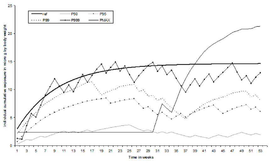
The cumulative individual exposure $S_{i,h,t}$ is calculated from the estimated individual weekly intakes according to equation $(\ref{Cumul_expo})$ and the resulting values for $t>35$ are compared to the reference cumulative exposure defined by $(\ref{cumul_ref})$. Figure 1 shows the cumulative individual exposure over the $53$ weeks of the year $2001$ for different individuals. Only certain percentiles of the distribution of the individual cumulative exposures of the last week are displayed. For example, the curve Pmax represents the cumulative exposure of an individual whose last week’s cumulative exposure is the highest. This is the cumulative exposure of a girl who turned one year old during the 30th week of 2001, lives in Paris or its suburbs in a well to do household. 

Very few individuals have a cumulative individual exposure above the reference long term exposure. We estimate that only $0.186\%$ of individuals are deemed at risk. This risk index should be compared to the more common one defined as the percentage of weekly intakes $D_{i,h,t}$ exceeding the PTWI, denoted $R_{1.6}$, such as $R_{1.6}=\frac{1}{nT}\sum_{t=1}^{T}\sum_{h=1}^{H}\sum_{i=1}^{n_{h}}1\mbox{l}\left(D_{i,h,t}>1.6\right)$. $R_{1.6}$ is equal to $0.45\%$, and is slightly higher since each occasional deviation above the PTWI increases the risk index whereas only long term deviations above this PTWI should be taken into account to assess the risk.

A deeper analysis of at risk individuals shows that all these vulnerable individuals are children less than three years old. They represent $5.29\%$ of the children aged between 1 and 3 in 2001. Further, no child of a modest households is found to be at risk.

Figure 1 around here, see page 1

4 Discussion

As mentioned in section 1, the use of household acquisition data in a food safety context, and in our case the use of the SECODIP database for assessing methylmercury dietary intakes, gives rise to some approximations:

1. Consumption outside of the home is out of the scope of household acquisition data. TNS SECODIP does not provide any information on the quantities of seafoods consumed out of the home or bought for outside consumption. Nevertheless, Serra-Majem et al. (2003) assert that these data are good estimates for the consumption of the whole household. Vasdekis and Trichopoulou (2000) avoid this question by using the term ”availaibility” instead of intake or consumption. However, as in Chesher (1997), auxiliary information about outdoor consumption could be introduced in the model as a correction factor accounting for the propensity to eat outside of the home according to age, sex or socioeconomic variables. The French INCA survey on individual consumptions gives details about inside / outside the home consumption for $3003$ individuals people aged 3 and older. The mean outside the home consumption proportion is $20\%$ for seafoods. Applying such a factor to all household intakes yields a long term risk of $0.226\%$, and $R_{1.6}=0.791\%$. Furthermore, in this case, a small proportion of consumers older than 3 years old are vulnerable. Nevertheless, children aged between 1 and 3 in 2001 still represent the most vulnerable consumer group, at $10\%$ of the corresponding population.

2. The amount of food bought by a household can be different from the amount actually consumed. Indeed, namely for seafoods, a non negligible part is not edible: Favier et al. (1995) show than on average only 61% of fresh or frozen fish is edible. Besides, Maresca and Poquet (1994) also demonstrate some part of the purchased food is thrown away, which also reduces the actual amount of food consumed by a household. However, SECODIP does not specify whether the quantity of fresh or frozen fish bought is ready to be consumed or as a whole fish that needs some preparation. Applying such a factor to all household intakes yields a long term risk of $0$.$00\%$, and $R_{1.6}=0.043\%$. If both the $20\%$ outside of the home consumption correction factor and the $61\%$ edible proportion factor are applied to our series, the long term risk is equal to $0.021\%$, $R_{1.6}=0.13\%$, and $1.06\%$ of the population of children aged between 1 and 3 are vulnerable. These results stress that applying such a correction factor to assess the actual quantity consumed is probably too strong and is certainly a crude approximation of the quantity of seafoods ingested. Thus, a more detailed database on fish and seafood is needed, to realize an accurate assessment of exposure to methylmercury, taking into account only the edible part of fish and other seafood.

   Body weight information is crucial in a food safety context and will be included in the future SECODIP data since it has now been added to the list of required individual characteristics. The measurement error afferent to this quantity will remain however, namely for children whose body weight changes a lot throughout a year. Nevertheless, approximating the weekly body weight of young children by the median of the weekly body weight distribution available in French health records is the best approximation possible.

3. The food nomenclature of the SECODIP database is not as detailed as the contamination database. Unfortunately, fish and seafood species are not well documented so it is not possible to consider more than two food categories when computing household intakes. This problem of nomenclature matching is ubiquitous of food risk assessments since contamination analysis are generally conducted independently from the food nomenclature of consumption data.

These arguments mainly show the disadvantages of the use of household food acquisition data such as the SECODIP database. Nevertheless, they also present many advantages compared to the individual food record survey mainly used in France in the food safety context:

• As mentioned before, households respond for a long period of time (the average is 4 years in the SECODIP panel) which allows us to observe long term behaviors and avoid some well known biases of individual food record surveys. For example, respondents might over- (under-) declare certain foods with a good (bad) nutritional value either deliberately or just because they increased (reduced) their consumption for the short (7 days) period of the survey.

• The individual surveys are expensive and very difficult to conduct. Highly trained interviewers are required and extraordinary cooperation is required from respondents. Household food acquisition data can serve many other applications (economics or marketing) and, at least for the SECODIP data, acquisition recording is simplified by optical scanning of food barcodes.

Conclusion

In this paper, we proposed a methodology to assess chronic risks related to food contamination using the example of methylmercury exposure through seafood consumption. This methodology includes the definition of a Kinetic Dietary Exposure Model (KDEM) that integrates the fact that contaminants are eliminated from the body at different rates, the rate being measured by the half life of the contaminant. In this paper, the estimation is based on the use of household food acquisition data which are first decomposed into individual intake data through a disaggregation model accounting for the dependence among household members. Several extensions of this methodology are currently studied. First, the disaggregation model could be improved by considering a preliminary step in which we determine what member is an actual consumer, in the spirit of the Tobit model. The KDEM idea is also currently being developed by studying the stability and ergodic properties of the underlying continuous time piecewise deterministic Markov process (Bertail et al., 2006). The parameters of this new model are the intake distribution, the inter intake time distribution and the dissipation rate distribution. In this framework, the dissipation parameter $\eta$ of the KDEM model is random and the intake and inter-intake distributions can be estimated either from individual (INCA-type) data or household (SECODIP-type) data.

Table 2: Restricted maximum likelihood estimates (REML) for age and all socioeconomic variables and the p-value of the Student’s tests (Pval)

Effect	Parameter	REML	Pval
Income	(ref: Mean sup)
Well to do	${\scriptsize\gamma}_{1}$	6.027	$<$0.001
Mean inf	${\scriptsize\gamma}_{2}$	2.686	$<$0.001
Modest	${\scriptsize\gamma}_{3}$	-1.928	$<$0.001
Region of residence	(ref: Noncoastal regions)
North, Brittany, Vendee coast	${\scriptsize\gamma}_{4}$	0.962	0.003
South West coast	${\scriptsize\gamma}_{5}$	5.232	$<$0.001
Mediterranean coast	${\scriptsize\gamma}_{6}$	2.303	$<$0.001
Paris and its suburbs	${\scriptsize\gamma}_{7}$	1.023	0.009
Occupation category of the principal household earner	(ref: Blue collar workers)
self-employed persons	${\scriptsize\gamma}_{8}$	-0.122	0.771
white collar workers	${\scriptsize\gamma}_{9}$	-3.733	$<$0.001
retirees	${\scriptsize\gamma}_{10}$	-5.261	$<$0.001
no activity	${\scriptsize\gamma}_{11}$	-1.910	0.004
Level of Education of the principal household earner	(ref: BAC and higher degree)
student	${\scriptsize\gamma}_{12}$	5.901	$<$0.001
no or weak diploma	${\scriptsize\gamma}_{13}$	-1.281	$<$0.001

Table 3: The different steps performed in testing the socioeconomic part of our model. For each step, the null hypothesis tested and the p-value resulting from the appropriate F-test are shown. All tests are performed conditionally on the results of the previous tests (Pval)

Null hypothesis	Pval
H1 : $\gamma_{8}=0$	0.771
H2 : $\gamma_{9}=\gamma_{10}$	0.030
H3 : $\gamma_{9}=\gamma_{11}$	0.018
H4 : $\gamma_{10}=\gamma_{11}$	$<$0.001
H5 : $\gamma_{4}=\gamma_{5}=\gamma_{6}=\gamma_{7}$	$<$0.001
H6 :  a : $\gamma_{4}=\gamma_{5}$	$<$0.001
b : $\gamma_{4}=\gamma_{6}$	$<$0.001
c : $\gamma_{4}=\gamma_{7}$	0.881
d : $\gamma_{5}=\gamma_{6}$	$<$0.001
e : $\gamma_{5}=\gamma_{7}$	$<$0.001
f : $\gamma_{6}=\gamma_{7}$	0.0103
H7 : $\gamma_{12}=\gamma_{13}$	$<$0.001
H8 : $\gamma_{1}=\gamma_{2}=\gamma_{3}$	$<$0.001
H9 : a : $\gamma_{1}=\gamma_{2}$	$<$0.001
b : $\gamma_{1}=\gamma_{3}$	$<$0.001
c : $\gamma_{2}=\gamma_{3}$	$<$0.001

Table 4: Restricted maximum likelihood estimates (REML) for all age and socioeconomic variables of the reduced final model with all variance components and their standard errors (s.e)

Effect	Parameter	REML	Pval
Income	(ref: Mean sup)
Well to do	${\scriptsize\gamma}_{1}$	6.108	$<$0.001
Mean inf	${\scriptsize\gamma}_{2}$	2.760	$<$0.001
Modest	${\scriptsize\gamma}_{3}$	-1.915	$<$0.001
Region of residence	(ref: Non coastal regions)
Paris and North, Brittany, Vendee coast	${\scriptsize\gamma}_{4}{\scriptsize=\gamma}_{7}$	0.995	$<$0.001
South west coast	${\scriptsize\gamma}_{5}$	5.156	$<$0.001
Mediterranean coast	${\scriptsize\gamma}_{6}$	2.250	$<$0.001
Occupation category of the principal household earner	(ref: Blue collar workers and self employed persons)
white collar workers	${\scriptsize\gamma}_{9}$	-3.745	$<$0.001
retirees	${\scriptsize\gamma}_{10}$	-5.243	$<$0.001
no activity	${\scriptsize\gamma}_{11}$	-1.871	0.005
Level of education of the principal household earner	(ref: BAC and higher degree)
student	${\scriptsize\gamma}_{12}$	5.879	$<$0.001
no or weak diploma	${\scriptsize\gamma}_{13}$	-1.279	$<$0.001
		REML	s.e
Variance of the random effect	${\scriptsize\sigma}_{u}$	24.832	6.7316
Variance-covariance structure
variance	${\scriptsize\sigma}^{{\scriptsize 2}}$	1260705	282309
correlation	${\scriptsize\rho}$	-0.22	0.0434

Figure 1: Cumulative exposure to MeHg (unit: $\mu$g per kg of body weight)

References

- (1)
- Bertail et al. (2006) Bertail, P., S. Clémençon and J. Tressou (2006). A storage model with random release rate for modeling exposure to food contaminants. Submitted for publication.
- Boizot (2005) Boizot, C. (2005). Présentation du panel de données SECODIP. Technical report. INRA-CORELA.
- Brumback et al. (1999) Brumback, B., D. Ruppert and M. P. Wand (1999). Comment on ”variable selection and function estimation in additive nonparametric regression using a data-based prior” by Shively, Kohn, and Wood. Journal of the American Statistical Association 94, 794–797.
- Chesher (1997) Chesher, A. (1997). Diet revealed?: Semiparametric estimation of nutrient intake-age relationships. Journal of the Royal Statistical Society A 160(3), 389–428.
- Chesher (1998) Chesher, A. (1998). Individual demands from household aggregates: Time and age variation in the quality of diet. Journal of Applied Econometrics 13(5), 505–524.
- Crainiceanu et al. (2003) Crainiceanu, C. M., D. Ruppert and T. J. Vogelsang (2003). Some properties of likelihood ratio tests in linear mixed models. (Working Paper).
- CREDOC-AFSSA-DGAL (1999) CREDOC-AFSSA-DGAL (1999). Enquête INCA (individuelle et nationale sur les consommations alimentaires). TEC&DOC ed.. Lavoisier, Paris. (Coordinateur : J.L. Volatier).
- Crépet et al. (2005) Crépet, A., J. Tressou, P. Verger and J. Ch. Leblanc (2005). Management options to reduce exposure to methyl mercury through the consumption of fish and fishery products by the French population. Regulatory Toxicology and Pharmacology 42(2), 179–189.
- Engle et al. (1986) Engle, R. F., C. W. J. Granger, J. Rice and A. Weiss (1986). Non-parametric estimation of the relationship between weather and electricity demand. Journal of the American Statistical Association 81, 310–320.
- FAO/WHO (2003) FAO/WHO (2003). Evaluation of certain food additives and contaminants for methylmercury. Sixty first report of the Joint FAO/WHO Expert Committee on Food Additives, Technical Report Series. WHO. Geneva, Switzerland.
- Favier et al. (1995) Favier, C., J. Ireland-Ripert, C. Toque and M. Feinberg (1995). R pertoire G n ral des Aliments, Table de composition, tome 1. TEC&DOC ed.. Lavoisier, Paris.
- Green and Silverman (1994) Green, P.J. and B.W. Silverman (1994). Nonparametric Regression and Generalized Linear Models. Chapman & Hall.
- Hamilton (1994) Hamilton, J. D. (1994). Time Series Analysis. Princeton University Press.
- Hoffmann et al. (2002) Hoffmann, K., H. Boeingand, A. Dufour, J. L. Volatier, J. Telman, M. Virtanen, W. Becker and S. De Henauw (2002). Estimating the distribution of usual dietary intake by short-term measurements. European Journal of Clinical Nutrition 56, 53–62.
- IFREMER (1994-1998) IFREMER (1994-1998). Résultat du réseau national d’observation de la qualité du milieu marin pour les mollusques (RNO).
- MAAPAR (1998-2002) MAAPAR (1998-2002). Résultats des plans de surveillance pour les produits de la mer. Ministère de l’Agriculture, de l’Alimentation, de la Pêche et des Affaires Rurales.
- Maresca and Poquet (1994) Maresca, B. and G. Poquet (1994). Collectes s lectives des d chets et comportements des m nages. Technical Report R146. CREDOC.
- Nusser et al. (1996) Nusser, S.M., A.L. A.L. Carriquiry, K.W. Dodd and W.A. Fuller (1996). A semiparametric transformation approach to estimating usual intake distributions. Journal of the American Statistical Association 91, 1440–1449.
- Patterson and Thompson (1971) Patterson, H. D. and R. Thompson (1971). Recovery of inter-block information when block sizes are unequal. Biometrika 58, 545–554.
- Ruppert et al. (2003) Ruppert, D., M .P. Wand and R. J. Carroll (2003). Semiparametric regression. Cambridge Series in Statistical and Probabilistic Mathematics. Cambrige University Press.
- Self and Liang (1987) Self, S. G. and K.Y. Liang (1987). Asymptotic properties of maximum likelihood estimators and likelihood ratio tests under nonstandard conditions. Journal of the American Statistical Association 82(398), 605–610.
- Sempé et al. (1979) Sempé, M., G. Pédron and M. P. Roy-Pernot (1979). Auxologie, méthode et séquences. Théraplix. Paris.
- Serra-Majem et al. (2003) Serra-Majem, L., D. MacLean, L. Ribas, D. Brule, W. Sekula, R. Prattala, R. Garcia-Closas, A. Yngve and M. Lalondeand A. Petrasovits (2003). Comparative analysis of nutrition data from national, household, and individual levels: results from a WHO-CINDI collaborative project in Canada, Finland, Poland, and Spain. Journal of Epidemiology and Community Health 57, 74–80.
- Smith and Farris (1996) Smith, J. C. and F. F. Farris (1996). Methyl mercury pharmacokinetics in man: A reevaluation. Toxicology And Applied Pharmacology 137, 245–252.
- Speed (1991) Speed, T. (1991). Discussion of “that blup is a good thing: the estimation of random effects” by g. robinson. Statistical science 6, 42–44.
- Tressou et al. (2004) Tressou, J., A. Crépet, P. Bertail, M. H. Feinberg and J. C. Leblanc (2004). Probabilistic exposure assessment to food chemicals based on extreme value theory. application to heavy metals from fish and sea products. Food and Chemical Toxicology 42(8), 1349–1358.
- Vasdekis and Trichopoulou (2000) Vasdekis, V.G.S. and A. Trichopoulou (2000). Non parametric estimation of individual food availability along with bootstrap confidence intervals in household budget surveys. Statistics and Probability Letters 46, 337–345.
- Verbyla (1999) Verbyla, A. (1999). Mixed Models for Practitioners. Biometrics SA, Adelaide.
- WHO (1990) WHO (1990). Methylmercury, environmental health criteria 101. Technical report. Geneva, Switzerland.
Figures and Tables