Temperature dependence of Coulomb drag between finite-length quantum wires

Abstract

We evaluate the Coulomb drag current in two finite-length Tomonaga-Luttinger-liquid wires coupled by an electrostatic backscattering interaction. The drag current in one wire shows oscillations as a function of the bias voltage applied to the other wire, reflecting interferences of the plasmon standing waves in the interacting wires. In agreement with this picture, the amplitude of the current oscillations is reduced with increasing temperature. This is a clear signature of non-Fermi-liquid physics because for coupled Fermi liquids the drag resistance is always expected to increase as the temperature is raised.

Coulomb drag phenomena in coupled one-dimensional (1D) electron systems have been investigated quite extensively in the past Flensberg (1998); Nazarov and Averin (1998); Komnik and Egger (1998); Gurevich et al. (1998); Klesse and Stern (2000); Ponomarenko and Averin (2000); Trauzettel et al. (2002); PusPRL03 ; Fiete et al. (2006); PusPRL06 . The interest has mainly been driven by the fact that Coulomb drag, i.e. the electrical response of one wire as a finite bias is applied to the other wire, seems to be an ideal testing ground for Tomonaga-Luttinger-liquid (TLL) physics in nature. This is because both inter-wire and intra-wire Coulomb interactions substantially modify transport properties such as the average current and the current noise. On the experimental side, there have been a few works, some of which have claimed to have observed TLL behavior in the drag data DebPHE00 ; DebJPCM01 ; Yamamoto et al. (2002). Recently, Yamamoto and coworkers have measured Coulomb drag in coupled quantum wires of different lengths and found peculiar transport properties that depend, for instance, on the asymmetry of the two wires Yamamoto et al. (2006). This experiment is the major motivation for our work.

We analyze theoretically the Coulomb drag current of two electrostatically coupled quantum wires using the concept of the inhomogeneous TLL model Maslov and Stone (1995); Ponomarenko (1995); Safi and Schulz (1995). This model is known to capture the essential physics of an interacting 1D wire of finite length coupled to non-interacting (Fermi liquid) electron reservoirs. Within this framework, we are able to study finite-length and finite-temperature effects and therefore to make qualitative contact with the experimental setup of Ref. Yamamoto et al. (2006). Since the Coulomb interaction varies between the wire regions and the lead regions, charge excitations feel the interaction difference at the boundaries and are known to exhibit Andreev-type reflections Safi and Schulz (1995). We show that these reflections play a crucial role in the Coulomb drag setup illustrated in Fig. 1. Furthermore, we show that the quantum interference phenomena associated with the Andreev-type reflections considerably modify the drag current. This is particularly interesting as far as the temperature dependence of the drag current is concerned. For Fermi-liquid systems, it is well known that the drag resistance should always increase as the temperature is raised Ponomarenko and Averin (2000). In our setup instead, the drag current at a fixed drive bias can either increase or decrease as a function of temperature. It crucially depends on the interference pattern due to finite-length effects. This is a clear signature of non-Fermi-liquid physics which could be observed in the double-wire setup of Ref. Yamamoto et al. (2006).

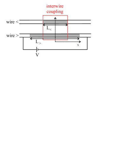
Figure 1: (color online). The system under consideration. Each interacting wire of length $L_{j}$ [gray area, interaction parameter $g_{j}({\left|x\right|}<L_{j}/2)=g_{j}<1$] is connected to a pair of non-interacting leads [$g_{j}({\left|x\right|}>L_{j}/2)=1$]. The region of backscattering inter-wire interaction (red dashed box) extends over the length of the shorter wire. A voltage $V$ is applied between the leads connected to the drive wire (here the longer wire $j={\mathrm{>}}$) and the backscattering-induced current $I_{\text{dr}}$ in the drag wire (here the shorter wire $j={\mathrm{<}}$) is investigated.

The system considered consists of two interacting parallel wires ($j={\mathrm{<}},{\mathrm{>}}$) of finite length $L_{\mathrm{<}}$ (shorter wire) and $L_{\mathrm{>}}$ (longer wire) connected to non-interacting semi-infinite 1D leads (Fig. 1) and is described by the Hamiltonian $H=\sum_{j={\mathrm{<}},{\mathrm{>}}}\left[H_{j}^{0}+H_{j}^{V}\right]+H_{\mathrm{C}}$. The intra-wire interaction is modelled through a TLL description Maslov and Stone (1995); Ponomarenko (1995); Safi and Schulz (1995)

$$H_{j}^{0}=\frac{\hbar v_{\mathrm{F}j}}{2}\int_{-\infty}^{\infty}\text{d}x\Bigl{[}\Pi_{j}^{2}+\frac{1}{g_{j}^{2}(x)}(\partial_{x}\Phi_{j})^{2}\Bigr{]}$$ (1)

with the piecewise constant interaction parameter $g_{j}(x)=g_{j}<1$ in the wire region ${\left|x\right|}<L_{j}/2$ and $g_{j}(x)=1$ in the non-interacting lead regions ${\left|x\right|}>L_{j}/2$. The Fermi velocity $v_{\mathrm{F}j}$, the interaction strength $g_{j}$, and the wire length $L_{j}$ set the frequency $\omega_{Lj}=v_{\mathrm{F}j}/g_{j}L_{j}$ of the collective plasmonic excitations hosted in each wire. A voltage $eV_{j}=\mu_{\mathrm{L}}^{(j)}-\mu_{\mathrm{R}}^{(j)}$ applied to the leads is described by

$$H_{j}^{V}=-\frac{1}{\sqrt{\pi}}\int_{-\infty}^{\infty}\text{d}x\ \mu_{j}(x)\partial_{x}\Phi_{j}(x),$$ (2)

with the piecewise constant electro-chemical potential

$$\mu_{j}(x)=\begin{cases}\mu_{\mathrm{L}}^{(j)}&\text{for $x<-L_{j}/2$},\\ 0&\text{ for ${\left|x\right|}<L_{j}/2$},\\ \mu_{\mathrm{R}}^{(j)}&\text{for $x>L_{j}/2$}\end{cases}$$ (3)

with $\mu_{\mathrm{L}}^{(j)}=-\mu_{\mathrm{R}}^{(j)}$. This model is expected to capture the essential physics of a quantum wire coupled smoothly to electron reservoirs (with typical smoothing length $L_{s}$) as long as $L_{j={\mathrm{<}},{\mathrm{>}}}\gg L_{s}\gg\lambda_{F}$, where $\lambda_{F}$ is the electron Fermi wavelength Dolcini et al. (2005); Enss05 . Finally, we include an inter-wire backscattering interaction over the length $L_{\mathrm{<}}$ of the shorter wire,

$$H_{\mathrm{C}}=\lambda_{\mathrm{BS}}\int_{-L_{\mathrm{<}}/2}^{L_{\mathrm{<}}/2}\text{d}x\ \cos\{\sqrt{4\pi}[\Phi_{\mathrm{<}}(x)-\Phi_{\mathrm{>}}(x)]\}.$$ (4)

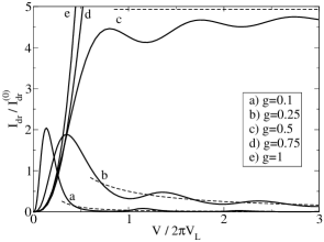
Figure 2: Drag current as a function of drive voltage for identical wires at zero temperature (solid curves). The inter-wire interaction strength ranges from strongly interacting ($g=0.1$) to non-interacting ($g=1$) for the different curves (with $I_{\mathrm{dr}}^{(0)}=e\lambda_{\mathrm{BS}}^{2}L^{2}\alpha^{4g}/\hbar^{2}\omega_{L}$ and $V_{L}=\hbar\omega_{L}/e$). The dashed curves show the dominant contribution $\propto V^{4g-2}$ [given in Eq. (10)] for $g=0.1,0.25,0.5$.

This term includes the contribution of the density-density interaction which is most relevant to Coulomb drag Flensberg (1998); Nazarov and Averin (1998) when the Fermi wave-vectors of both wires are similar in magnitude, i.e. $k_{\mathrm{F}{\mathrm{<}}}\approx k_{\mathrm{F}{\mathrm{>}}}$ .

In the following, we choose to apply a voltage $V_{\mathrm{>}}=V$ to the longer wire ($\mu_{\mathrm{L}}^{{\mathrm{>}}}=-\mu_{\mathrm{R}}^{{\mathrm{>}}}=eV/2$, drive wire) and none $V_{\mathrm{<}}=0$ to the shorter wire ($\mu_{\mathrm{L}}^{{\mathrm{<}}}=\mu_{\mathrm{R}}^{{\mathrm{<}}}=0$, drag wire). The average current in the wires may then be written as $I_{\mathrm{<}}=I_{\mathrm{dr}}$ and $I_{\mathrm{>}}=\frac{e^{2}}{h}V-I_{\mathrm{dr}}$. In our model, the two currents $I_{\mathrm{<}}$ and $I_{\mathrm{>}}$ always flow in the same direction, which is due to momentum conservation. This is known as positive Coulomb drag.

In order to get an expression for the drag current $I_{\mathrm{dr}}$, we follow the formalism used in Dolcini et al. (2005) in the case of a single wire with an impurity. We consider the situation of weak inter-wire coupling. To second order in $\lambda_{\mathrm{BS}}$, we obtain

$$I_{\mathrm{dr}}=I_{\mathrm{dr}}^{(0)}\int_{0}^{1}\text{d}R\int_{0}^{1-R}\text{d}rj_{\mathrm{dr}}(r,R),$$ (5)

with the normalization $I_{\mathrm{dr}}^{(0)}={e\lambda_{\mathrm{BS}}^{2}L_{\mathrm{<}}^{2}\alpha_{\mathrm{<}}^{4g_{\mathrm{<}}}}/{\hbar^{2}\omega_{L{\mathrm{<}}}}$, where $\alpha_{\mathrm{<}}=\omega_{L{\mathrm{<}}}/\omega_{\mathrm{c}}$ is the ratio between the plasmon frequency of the shorter wire and a cutoff frequency $\omega_{\mathrm{c}}$, of the order of the wire bandwidth. The plasmon frequency defines a voltage $V_{L}=\hbar\omega_{L{\mathrm{<}}}/e$ and a temperature $T_{L}=\hbar\omega_{L{\mathrm{<}}}/k_{\mathrm{B}}$. It is convenient to introduce corresponding dimensionless voltage $u=V/V_{L}$ and temperature $\theta=T/T_{L}$. The integrand in (5),

$$j_{\mathrm{dr}}(r,R)=\frac{1}{2\alpha_{\mathrm{<}}^{4g_{\mathrm{<}}}}\int_{-\infty}^{\infty}\text{d}\tau\left(\text{e}^{\text{i}u\tau}-\text{e}^{-\text{i}u\tau}\right)\\ \times\exp\left[4\pi C_{\mathrm{<}}(r,R;\tau)+4\pi C_{\mathrm{>}}\left(\frac{r}{l},\frac{R}{l};\frac{q\tau}{pl}\right)\right],$$ (6)

involves the parameters $l=L_{\mathrm{>}}/L_{\mathrm{<}}$, $p=g_{\mathrm{>}}/g_{\mathrm{<}}$, and $q=v_{\mathrm{F}{\mathrm{>}}}/v_{\mathrm{F}{\mathrm{<}}}$. The correlation function $C_{j}=C_{j}^{\mathrm{GS}}+C_{j}^{\mathrm{TF}}$ of each wire can be decomposed in a zero-temperature and a finite-temperature contribution given by Dolcini et al. (2005)

$$C_{j}^{\mathrm{GS}}(r,R;\tau)=-\frac{g_{j}}{4\pi}\sum_{\begin{subarray}{c}k\in\mathbb{Z}\\ s=\pm\end{subarray}}\biggl{[}\gamma_{j}^{\left|2k\right|}\ln\biggl{(}\frac{\alpha_{j}+\text{i}(\tau-sr-2k)}{\alpha_{j}+\text{i}(-2k)}\biggr{)}+\gamma_{j}^{\left|2k+1\right|}\ln\biggl{(}\frac{\alpha_{j}+\text{i}(\tau-sR-2k-1)}{[\alpha_{j}^{2}+(r-sR-2k-1)^{2}]^{1/2}}\biggr{)}\biggl{]},$$ (7)

$$C_{j}^{\mathrm{TF}}(r,R;\tau)=-\frac{g_{j}}{4\pi}\sum_{\begin{subarray}{c}k\in\mathbb{Z}\\ s=\pm\end{subarray}}\biggl{[}\gamma_{j}^{\left|2k\right|}\ln\biggl{(}\frac{\mathop{\text{sinch}}[\pi\theta(\tau-sr-2k)]}{\mathop{\text{sinch}}[\pi\theta(-2k)]}\biggr{)}+\gamma_{j}^{\left|2k+1\right|}\ln\biggl{(}\frac{\mathop{\text{sinch}}[\pi\theta(\tau-sR-2k-1)]}{\mathop{\text{sinch}}[\pi\theta(r-sR-2k-1)]}\biggr{)}\biggr{]},$$ (8)

with $\gamma_{j}=(1-g_{j})/(1+g_{j})$ and $\mathop{\text{sinch}}x=(\sinh x)/x$.

It is to be noted that the expression for the drag current $I_{\mathrm{dr}}$ does not depend on whether the drive wire is the longer wire or the shorter one due to the symmetry of our model. In the following, we present results obtained by numerical evaluation of the triple integral involved in (5) and (6) and discuss several analytical approximations.

First we set the temperature to zero and consider identical wires ($l=p=q=1$, thus we drop the wire index $j$). The drag current shows non-monotonous behavior and oscillations with period $\sim 2\pi\hbar\omega_{L}/e$ as a function of the bias voltage (Fig. 2). It decays at large voltages for $g<1/2$ whereas it increases for $g>1/2$. Thus, we obtain qualitatively the same behavior as in a dual Coulomb drag setup where a drive current is applied and a drag voltage is measured Nazarov and Averin (1998). Similar oscillations as a function of voltage have been predicted in the context of two coupled fractional quantum Hall line junctions zuel04 .

An analytic approximation can be derived in the limit $u=eV/\hbar\omega_{L}\gg 1$, that is for high voltages or long wires. In Eq. (7), the terms proportional to $\gamma^{{\left|m\right|}}$ account for contributions from plasmon excitations reflected ${\left|m\right|}$ times inside the wire. When the wire length is much longer than other relevant length scales, the contribution without any reflection $m=0$ becomes dominant and yields the integrand

$$j_{\mathrm{dr}}(r,R)\underset{u\gg 1}{\sim}\frac{\pi^{3/2}}{\Gamma(2g)}\left(\frac{u}{2r}\right)^{2g-1/2}J_{2g-1/2}(ur),$$ (9)

where $\Gamma(z)$ denotes the Gamma function and $J_{\nu}(z)$ the Bessel function of order $\nu$. The resulting expression for the drag current, which involves hypergeometric functions, underestimates the amplitude of the oscillations with respect to the exact numerical result. However, the behavior at large $u$, governed by the dominant contribution

$$I_{\mathrm{dr}}\underset{u\gg 1}{\sim}I_{\mathrm{dr}}^{(0)}\frac{\pi^{2}}{2\Gamma^{2}(2g)}\left(\frac{u}{2}\right)^{4g-2},$$ (10)

shows good agreement in the appropriate parameter regime (dashed curves in Fig. 2). Since we do perturbation theory in $\lambda_{\rm BS}$, the relation $I_{\mathrm{dr}}\ll(e^{2}/h)V$ has to hold. In the large $u$ regime, this means $(\lambda_{\rm BS}L/\hbar\omega_{c})^{2}(\omega_{L}/\omega_{c})(eV/\hbar\omega_{c})^{4g-3}\ll 1$.

Now we consider the situation where the two wires have different lengths. The qualitative behavior of the drag current does not change for increasing length ratio $l=L_{\mathrm{>}}/L_{\mathrm{<}}$, but the peak positions get shifted to lower voltages (Fig. 3). Here, neglecting plasmon reflections in the correlation function of the wires leads again to the expression (9), which is independent of $l$. This fact explains why the drag current does not change appreciably as a function of $l$ and indicates that the peak shifts observed result from plasmon reflections inside the wires. Our studies are the first to analyze the effect of an asymmetry in the length on Coulomb drag phenomena in coupled quantum wires which is of recent experimental relevance Yamamoto et al. (2006).

We now discuss in detail the temperature dependence of the drag current. For clarity, we consider again symmetric wires ($l=1$) . The oscillations of the drag current as a function of bias voltage get washed out with increasing temperature (Fig. 4). This behavior is consistent with the picture which attributes the oscillations to interferences of the plasmon excitations of the wires. Thus, for bias voltages such that the drag current is close to a maximum at zero temperature, one observes a decrease of the drag current with increasing temperature, whereas the opposite behavior can be observed close to a minimum of the zero-temperature drag current for strong interactions. This behavior is in stark contrast to the linear temperature dependence predicted for Coulomb drag between 1D Fermi-liquid conductors Gurevich et al. (1998) and therefore a clear signature of TLL physics. Note that our Fig. 4 bears significant resemblance to Fig. 9 of Ref. DebJPCM01 .

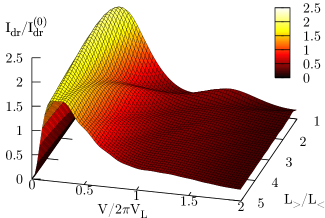
Figure 3: (color online). Drag current as a function of the bias voltage and of the length ratio of the wires (with $I_{\mathrm{dr}}^{(0)}=e\lambda_{\mathrm{BS}}^{2}L_{\mathrm{<}}^{2}\alpha_{\mathrm{<}}^{4g}/\hbar^{2}\omega_{L{\mathrm{<}}}$ and $V_{L}=\hbar\omega_{L{\mathrm{<}}}/e$).

A good approximation of the drag current can be obtained for temperatures much larger than the temperature associated with the plasmon frequency, $\theta=k_{\mathrm{B}}T/\hbar\omega_{L}\gg 1$, by neglecting contributions from plasmon reflections in the wires. Then, we obtain the dominant contribution

$$I_{\mathrm{dr}}\underset{\theta\gg 1}{\sim}I_{\mathrm{dr}}^{(0)}(2\pi\theta)^{4g-2}\sinh\left(\frac{u}{2\theta}\right)\frac{{\left|\Gamma\left(g+\frac{\text{i}u}{4\pi\theta}\right)\right|}^{4}}{4\Gamma^{2}(2g)}.$$ (11)

Taking the limit of low bias voltage in this result,

$$I_{\mathrm{dr}}\underset{\theta\gg 1,u}{\sim}I_{\mathrm{dr}}^{(0)}\frac{\pi\Gamma^{4}(g)}{4\Gamma^{2}(2g)}(2\pi\theta)^{4g-3}u,$$ (12)

we recover the power-law dependence $T^{4g-3}$ of the linear conductance predicted by renormalization group analysis Klesse and Stern (2000). At large bias voltage $u\gg\theta\gg 1$, we recover the zero-temperature result (10).

In the case $g=1/2$, Eq. (11) as well as the contribution to next order in $\theta^{-1}$ can be brought into a compact analytic form

$$I_{\mathrm{dr}}\underset{\theta\gg 1}{\sim}I_{\mathrm{dr}}^{(0)}\biggl{[}\frac{\pi^{2}}{2}\tanh\left(\frac{u}{4\theta}\right)\\ +\frac{1}{4\theta}\mathop{\text{Im}}\left\{\Psi^{\prime}\left(\frac{1}{2}+\frac{\text{i}u}{4\pi\theta}\right)\right\}\biggr{]},$$ (13)

where $\Psi^{\prime}(z)=\text{d}^{2}\ln\Gamma(z)/\text{d}z^{2}$ denotes the trigamma function. The first term is Eq. (11) evaluated at $g=1/2$ (dotted curve in Fig. 5), and the second one is the dominant correction, which takes values within $[-I_{\mathrm{dr}}^{(0)}/\theta,0]$ (included in the dashed curve in Fig. 5). This illustrates that the first-order approximation already yields a nice qualitative description for the full numerical result, which makes us confident that Eq. (11) is a good high-temperature approximation also for $g\neq 1/2$.

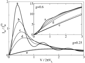
Figure 4: Temperature dependence of the drag current for identical wires with interaction strength $g=0.25$. The solid curves (labelled a - e) are evaluated for temperatures given by $T/T_{L}=k_{\mathrm{B}}T/\hbar\omega_{L}=0,0.5,1,1.5,5$, respectively (with $I_{\mathrm{dr}}^{(0)}=e\lambda_{\mathrm{BS}}^{2}L^{2}\alpha^{4g}/\hbar^{2}\omega_{L}$ and $V_{L}=\hbar\omega_{L}/e$). The dashed curve shows the high-temperature limit (11) for $T/T_{L}=5$. The inset shows a similar plot for weaker intra-wire interaction $g=0.6$ where the oscillations are less pronounced.

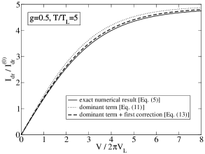
Figure 5: Drag current at high temperature ($T/T_{L}=5$) for identical wires with interaction strength $g=0.5$ (solid curve), where $I_{\mathrm{dr}}^{(0)}=e\lambda_{\mathrm{BS}}^{2}L^{2}\alpha^{4g}/\hbar^{2}\omega_{L}$ and $V_{L}=\hbar\omega_{L}/e$. The dotted curve shows the dominant contribution in the high-temperature limit [first term in (13)], the dashed curve includes the first correction as well [both terms in (13)].

In summary, we have analyzed two coupled quantum wires that exhibit both a finite intra-wire interaction and a finite inter-wire interaction. We have taken into account finite-length effects within the inhomogeneous TLL model that is known to capture the essential physics of quantum wires coupled to Fermi-liquid reservoirs. We have investigated how an asymmetry in the lengths of the wires changes the drag current and we have predicted a rich temperature dependence of the drag current that shows clear signatures of non-Fermi-liquid physics.

We would like to thank F. Dolcini, H. Grabert, M. Kindermann, Y. Nazarov, S. Tarucha, and M. Yamamoto for interesting discussions. This work was supported by the Swiss NSF and the NCCR Nanoscience.

References

- Flensberg (1998) K. Flensberg, Phys. Rev. Lett. 81, 184 (1998).
- Nazarov and Averin (1998) Y. V. Nazarov and D. V. Averin, Phys. Rev. Lett. 81, 653 (1998).
- Komnik and Egger (1998) A. Komnik and R. Egger, Phys. Rev. Lett. 80, 2881 (1998).
- Gurevich et al. (1998) V. L. Gurevich, V. B. Pevzner, and E. W. Fenton, J. Phys.: Condens. Matter 10, 2551 (1998).
- Klesse and Stern (2000) R. Klesse and A. Stern, Phys. Rev. B 62, 16912 (2000).
- Ponomarenko and Averin (2000) V. V. Ponomarenko and D. V. Averin, Phys. Rev. Lett. 85, 4928 (2000).
- Trauzettel et al. (2002) B. Trauzettel, R. Egger, and H. Grabert, Phys. Rev. Lett. 88, 116401 (2002).
- (8) M. Pustilnik, E. G. Mishchenko, L. I. Glazman, and A. V. Andreev, Phys. Rev. Lett. 97, 126805 (2003).
- Fiete et al. (2006) G. A. Fiete, K. Le Hur, and L. Balents, Phys. Rev. B 73, 165104 (2006).
- (10) M. Pustilnik, E. G. Mishchenko, and O. A. Starykh, Phys. Rev. Lett. 97, 246803 (2006).
- (11) P. Debray et al., Physica E 6, 694 (2000).
- (12) P. Debray et al., J. Phys.: Condens. Matter 13, 3389 (2001).
- Yamamoto et al. (2002) M. Yamamoto, M. Stopa, Y. Tokura, Y. Hirayama, and S. Tarucha, Physica E 12, 726 (2002).
- Yamamoto et al. (2006) M. Yamamoto, M. Stopa, Y. Tokura, Y. Hirayama, and S. Tarucha, Science 313, 204 (2006).
- Maslov and Stone (1995) D. L. Maslov and M. Stone, Phys. Rev. B 52, R5539 (1995).
- Ponomarenko (1995) V. V. Ponomarenko, Phys. Rev. B 52, R8666 (1995).
- Safi and Schulz (1995) I. Safi and H. J. Schulz, Phys. Rev. B 52, R17040 (1995).
- Dolcini et al. (2005) F. Dolcini, B. Trauzettel, I. Safi, and H. Grabert, Phys. Rev. B 71, 165309 (2005).
- (19) The effect of a finite smoothing length on the conductance in an equivalent model has been analyzed by K. Janzen, V. Meden, and K. Schönhammer, Phys. Rev. B 74, 085301 (2006).
- (20) U. Zülicke and E. Shimshoni, Phys. Rev. B 69, 085307 (2004).
- Komnik and Egger (2001) A. Komnik and R. Egger, Eur. Phys. J. B 19, 271 (2001).