On universality of critical behaviour in the focusing nonlinear Schrödinger equation, elliptic umbilic catastrophe and the tritronquée solution to the Painlevé-I equation.

Abstract

We argue that the critical behaviour near the point of “gradient catastrophe” of the solution to the Cauchy problem for the focusing nonlinear Schrödinger equation $i\epsilon\,\Psi_{t}+\frac{\epsilon^{2}}{2}\Psi_{xx}+|\Psi|^{2}\Psi=0$, $\epsilon\ll 1$, with analytic initial data of the form $\Psi(x,0;\epsilon)=A(x)\,e^{\frac{i}{\epsilon}S(x)}$ is approximately described by a particular solution to the Painlevé-I equation.

1 Introduction

The focusing nonlinear Schrödinger (NLS) equation for the complex valued function $\Psi=\Psi(x,t)$

$$i\,\Psi_{t}+\frac{1}{2}\Psi_{xx}+|\Psi|^{2}\Psi=0$$ (1.1)

has numerous physical applications in the description of nonlinear waves (see, e.g., the books [47, 35, 36]). It can be considered as an infinite dimensional analogue of a completely integrable Hamiltonian system [48], where the Hamiltonian and the Poisson bracket is given by

$$\Psi_{t}+\{\Psi(x),{\cal H}\}=0$$

$$\{\Psi(x),\Psi^{*}(y)\}=i\,\delta(x-y)$$ (1.2)

$${\cal H}=\frac{1}{2}\,\int\left(|\Psi_{x}|^{2}-|\Psi\ |^{4}\right)\,dx$$

(here $\Psi^{*}$ stands for the complex conjugate function). Properties of various classes of solutions to this equation have been extensively studied both analytically and numerically [5, 6, 7, 8, 16, 21, 25, 26, 29, 32, 34, 43, 44]. One of the striking features that distinguishes this equation from, say, the defocusing case

$$i\,\Psi_{t}+\frac{1}{2}\Psi_{xx}-|\Psi|^{2}\Psi=0$$

is the phenomenon of modulation instability [1, 11, 16]. Namely, slow modulations of the plane wave solutions

$$\Psi=A\,e^{i(kx-\omega t)},\quad\omega=\frac{1}{2}\,k^{2}-A^{2}$$

develop fast oscillations in finite time.

The appropriate mathematical framework for studying these phenomena is the theory of the initial value problem

$$\Psi(x,0;\epsilon)=A(x)\,e^{\frac{i}{\epsilon}S(x)}$$ (1.3)

for the $\epsilon$-dependent NLS

$$i\,\epsilon\,\Psi_{t}+\frac{\epsilon^{2}}{2}\Psi_{xx}+|\Psi|^{2}\Psi=0.$$ (1.4)

Here $\epsilon>0$ is a small parameter, $A(x)$ and $S(x)$ are real-valued smooth functions. Introducing the slow variables

$$u=|\Psi|^{2},\quad v=\frac{\epsilon}{2i}\left(\frac{\Psi_{x}}{\Psi}-\frac{\Psi_{x}^{*}}{\Psi^{*}}\right)$$ (1.5)

the equation can be recast into the following system:

$$u_{t}+(u\,v)_{x}=0$$

(1.6)

$$v_{t}+v\,v_{x}-u_{x}+\frac{\epsilon^{2}}{4}\left(\frac{1}{2}\frac{u_{x}^{2}}{u^{2}}-\frac{u_{xx}}{u}\right)_{x}=0.$$

The initial data for the system (1) coming from (1.3) do not depend on $\epsilon$:

$$u(x,0)=A^{2}(x),\quad v(x,0)=S^{\prime}(x).$$ (1.7)

The simplest explanation of the modulation instability then comes from considering the so-called dispersionless limit $\epsilon\to 0$. In this limit one obtains the following first order quasilinear system

$$\left.\begin{array}[]{lr}u_{t}&+v\,u_{x}+u\,v_{x}=0\\ &\\ v_{t}&-~{}~{}u_{x}+v\,v_{x}=0\end{array}\right\}.$$ (1.8)

This is a system of elliptic type because of the condition $u>0$. Indeed, the eigenvalues of the coefficient matrix

$$\left(\begin{array}[]{cc}v&u\\ -1&v\end{array}\right)$$

are complex conjugate, $\lambda=v\pm i\sqrt{u}$. So, the Cauchy problem for the system (1.8) is ill-posed in the Hadamard sense (cf. [33, 7]). Even for analytic initial data the life span of a typical solution is finite, $t<t_{0}$. The $x$- and $t$-derivatives explode at some point $x=x_{0}$ when the time approaches $t_{0}$. This phenomenon is similar to the gradient catastrophe of solutions to nonlinear hyperbolic PDEs [2].

For the full system (1) the Cauchy problem is well-posed for a suitable class of $\epsilon$-independent initial data (see details in [17, 46]). However, the well-posedness is not uniform in $\epsilon$. In practical terms that means that the solution to (1) behaves in a very irregular way in some regions of the $(x,t)$-plane when $\epsilon\to 0$. Such an irregular behaviour begins near the points $(x=x_{0},t=t_{0})$ of the “gradient catastrophe” of the solution to the dispersionless limit (1.8). The solutions to (1.8) and (1) are essentially indistinguishable for $t<t_{0}$; the situation changes dramatically near $x_{0}$ when approaching the critical point. Namely, when approaching $t=t_{0}$ the peak near a local maximum of $u$ becomes more and more narrow due to self-focusing; the solution develops a zone of rapid oscillations for $t>t_{0}$. They have been studied both analytically and numerically in [8, 16, 21, 23, 25, 26, 34, 43, 44]. However, no results are available so far about the behaviour of the solutions to the focusing NLS at the critical point $(x_{0},t_{0})$.

The main subject of this work is the study of the behaviour of solutions to the Cauchy problem (1), (1.7) near the point of gradient catastrophe of the dispersionless system (1.8). In order to deal with the Cauchy problem for (1.8) we will assume analyticity of the initial data $u(x,0)$, $v(x,0)$. Then the Cauchy problem for (1.8) can be solved for $t<t_{0}$ via a suitable version of the hodograph transform (see Section 2 below). An important feature of the gradient catastrophe for this system is that it happens at an isolated point of the $(x,t)$-plane, unlikely the case of KdV or defocusing NLS where the singularity of the hodograph solution takes place on a curve. We identify this singularity for a generic solution to (1.8) as the elliptic umbilic singularity (see Section 4 below) in the terminology of R.Thom [42]. This codimension 2 singularity is one of the real forms labeled by the root system of the $D_{4}$ type in the terminology of V.Arnold et al. [3].

Our main goal is to find a replacement for the elliptic umbilic singularity when the dispersive terms are added, i.e., we want to describe the leading term of the asymptotic behaviour for $\epsilon\to 0$ of the solution to (1) near the critical point $(x_{0},t_{0})$ of a generic solution to (1.8).

Thus, our study can be considered as a continuation of the programme initiated in [13] to study critical behaviour of Hamiltonian perturbations of nonlinear hyperbolic PDEs; the fundamental difference is that the non perturbed system (1.8) is not hyperbolic! However, many ideas and methods of [13] (see also [12]) play an important role in our considerations.

The most important of these is the idea of universality of the critical behaviour. The general formulation of the universality suggested in [13] for the case of Hamiltonian perturbations of the scalar nonlinear transport equation says that the leading term of the multiscale asymptotics of the generic solution near the critical point does not depend on the choice of the solution, modulo Galilean transformations and rescalings. This leading term was identified in [13] via a particular solution to the fourth order analogue of the Painlevé-I equation (the so-called $P_{1}^{2}$ equation). The existence of the needed solution to $P_{1}^{2}$ has been rigorously established in [9]. Moreover, it was argued in [13] that this behaviour is essentially independent on the choice of the Hamiltonian perturbation. Some of these universality conjectures have been partially confirmed by numerical analysis carried out in [21].

The main message of this paper is the formulation of the Universality Conjecture for the critical behaviour of the solutions to the focusing NLS. Our considerations suggest the description of the leading term in the asymptotic expansion of the solution to (1) near the critical point via a particular solution to the classical Painlevé-I equation (P-I)

$$\Omega_{\zeta\zeta}=6\,\Omega^{2}-\zeta.$$

The so-called tritronquée solution to P-I was discovered by P.Boutroux [4] as the unique solution having no poles in the sector $|\arg\zeta|<4\pi/5$ for sufficiently large $|\zeta|$. Remarkably, the very same solution arises in the critical behaviour of solutions to focusing NLS!

The paper is organized as follows. In Section 2 we develop a version of the hodograph transform for integrating the dispersionless system (1.8) before the catastrophe $t<t_{0}$. We also establish the shape of the singularity of the solution near the critical point; the latter is identified in Section 4 with the elliptic umbilic catastrophe of Thom. In Section 3 we develop a method of constructing formal perturbative solutions to the full system (1) before the critical time. In Section 5 we collect the necessary information about the tritronquée solution of P-I and formulate the Main Conjecture of this paper. Such a formulation relies on a much stronger property of the tritronquée solution: namely, we need this solution to be pole-free in the whole sector $|\arg\zeta|<4\pi/5$. Numerical evidence for the absence of poles in this sector is given in Section 6. In Section 7 we analyze numerically the agreement between the critical behaviour of solutions to focusing NLS and its conjectural description in terms of the tritronquée solution restricted on certain lines in the complex $\zeta$-plane. In the final Section 8 we give some additional remark and outline the programme of future research.

Acknowledgments. The authors thank K.McLaughlin for a very instructive discussion. One of the authors (B.D.) thanks R.Conte for bringing his attention to the tritronquées solutions of P-I. The results of this paper have been presented by one of the authors (T.G.) at the Conference “The Theory of Highly Oscillatory Problems”, Newton Institute, Cambridge, March 26 - 30, 2007. T.G. thanks A.Fokas and S.Venakides for the stimulating discussion after the talk. The present work is partially supported by the European Science Foundation Programme “Methods of Integrable Systems, Geometry, Applied Mathematics” (MISGAM), Marie Curie RTN “European Network in Geometry, Mathematical Physics and Applications” (ENIGMA). The work of B.D. and T.G. is also partially supported by Italian Ministry of Universities and Researches (MUR) research grant PRIN 2006 “Geometric methods in the theory of nonlinear waves and their applications”.

2 Dispersionless NLS, its solutions and critical behaviour

The equations (1) are a Hamiltonian system

$$\left.\begin{array}[]{r}u_{t}+\{u(x),H\}=0\\ \\ v_{t}+\{v(x),H\}=0\end{array}\right\}$$

with respect to the Poisson bracket originated in (1)

$$\{u(x),v(y)\}=\delta^{\prime}(x-y),$$ (2.1)

other brackets vanish, with the Hamiltonian

$$H=\int\left[\frac{1}{2}\left(u\,v^{2}-u^{2}\right)+\frac{\epsilon^{2}}{8u}u_{x}^{2}\right]\,dx.$$ (2.2)

Let us first describe the general analytic solution to the dispersionless system (1.8).

Lemma 2.1

Let $u_{I}(x)$, $v_{I}(x)$ be two real valued analytic functions of the real variable $x$ satisfying

$$\left(u_{I,x}\right)^{2}+\left(v_{I,x}\right)^{2}\neq 0.$$

Then the solution $u=u(x,t)$, $v=v(x,t)$ to the Cauchy problem

$$u(x,0)=u_{I}(x),\quad v(x,0)=v_{I}(x)$$ (2.3)

for the system (1.8) for sufficiently small $t$ can be determined from the following system

$$\left.\begin{array}[]{l}x=v\,t+f_{u}\\ \\ 0=u\,t+f_{v}\end{array}\right\}$$ (2.4)

where $f=f(u,v)$ is an analytic solution to the following linear PDE:

$$f_{vv}+u\,f_{uu}=0.$$ (2.5)

Conversely, given any solution to (2.5) satisfying $u^{2}f_{uu}^{2}+f_{uv}^{2}\neq 0$ at some point $(u=\tilde{u},v=\tilde{v})$ such that $f_{v}(\tilde{u},\tilde{v})=0$, the system (2.4) determines a solution to (1.8) defined locally near the point $x=\tilde{x}:=f_{u}(\tilde{u},\tilde{v})$ for sufficiently small $t$.

Remark 2.2

The solutions to the linear PDE (2.5) correspond to the first integrals of dispersionless NLS:

$$F=\int f(u,v)\,dx,\quad\frac{d}{dt}F=0.$$ (2.6)

Taking them as the Hamiltonians

$$\left.\begin{array}[]{r}u_{s}+\{u(x),F\}\equiv u_{t}+\left(f_{v}\right)_{x}=0\\ \\ v_{s}+\{v(x),F\}\equiv v_{t}+\left(f_{u}\right)_{x}=0\end{array}\right\}$$ (2.7)

yields infinitesimal symmetries of the dispersionless NLS:

$$\left(u_{t}\right)_{s}=\left(u_{s}\right)_{t},\quad\left(v_{t}\right)_{s}=\left(v_{s}\right)_{t}.$$ (2.8)

One of the first integrals will be extensively used in this paper. It corresponds to the Hamiltonian density

$$g=-\frac{1}{2}v^{2}+u(\log u-1).$$ (2.9)

The associated Hamiltonian flow reads

$$\left.\begin{array}[]{r}u_{s}+v_{x}=0\\ \\ v_{s}=\frac{u_{x}}{u}\end{array}\right\}$$ (2.10)

Eliminating the dependent variable $v$ one arrives at the elliptic version of the long wave limit of Toda lattice:

$$u_{ss}+\left(\log u\right)_{xx}=0.$$

Due to commutativity (2.8) the systems (1.8) and (2.10) admit a simultaneous solution $u=u(x,t,s)$, $v=v(x,t,s)$. Any such solution can be locally determined from a system similar to (2.4)

$$\left.\begin{array}[]{l}x=v\,t+f_{u}\\ \\ s=u\,t+f_{v}\end{array}\right\}$$ (2.11)

where $f=f(u,v)$, as above, solves the linear PDE (2.5).

The system (2.11) determines a solution $u=u(x,t,s)$, $v=v(x,t,s)$ provided applicability of the implicit function theorem. The conditions of the latter fail to hold at the critical point $(x_{0},s_{0},t_{0},u_{0},v_{0})$ such that

$$\begin{array}[]{l}x_{0}=v_{0}t_{0}+f_{u}(u_{0},v_{0})\\ \\ s_{0}=u_{0}t_{0}+f_{v}(u_{0},v_{0})\\ \\ f_{uu}(u_{0},v_{0})=f_{vv}(u_{0},v_{0})=0,\quad f_{uv}(u_{0},v_{0})=-t_{0}\end{array}$$ (2.12)

In sequel we adopt the following system of notations: the values of the function $f$ and of its derivatives at the critical point will be denoted by $f^{0}$ etc. E.g., the last line of the conditions (2.12) will read

$$f_{uu}^{0}=f_{vv}^{0}=0,\quad f_{uv}^{0}=-t_{0}.$$

Definition 1. We say that the critical point is generic if at this point:

$$f_{uuv}^{0}\neq 0.$$

Let us the introduce real parameters $r$, $\psi$ determined by the third derivatives of the function $f$ evaluated at the critical point,

$$\frac{1}{r}(\cos\psi-i\sin\psi)=f_{uuv}^{0}+i\sqrt{u_{0}}f_{uuu}^{0}.$$ (2.13)

Due to the genericity assumption

$$\psi\neq\frac{\pi}{2}+\pi k.$$

In order to describe the local behaviour of a solution to the dispersionless NLS/Toda equations we define a function $R(X;S,\psi)$ of real variables $X$, $S$ depending on the real parameter $\psi$ satisfying

$$(S+\cos\psi)^{2}+(X+\sin\psi)^{2}\neq 0$$ (2.14)

by the following formula

$$R(X,S,\psi)=\mbox{sign}\hskip 1.42262pt[\cos{\psi}]$$ (2.15)

$$\times\sqrt{1+X\sin{\psi}+S\cos{\psi}+\sqrt{1+2(X\sin{\psi}+S\cos{\psi})+X^{2}+S^{2}}}$$

Put

$$P_{0}(X,S,\psi)=\frac{1}{\sqrt{2}}\left[R(X,S,\psi)\cos{\psi}-\frac{(X\cos{\psi}-S\sin{\psi})\sin{\psi}}{R(X,S,\psi)}\right]-\cos{\psi}$$

(2.16)

$$Q_{0}(X,S,\psi)=\frac{1}{\sqrt{2}}\left[\frac{(X\cos{\psi}-S\sin{\psi})\cos{\psi}}{R(X,S,\psi)}+R(X,S,\psi)\sin{\psi}\right]-\sin{\psi}.$$

Observe that $P_{0}(X,S,\psi)$ and $Q_{0}(X,S,\psi)$ are smooth functions of the real variable $X$ provided validity of the inequality (2.14).

Lemma 2.3

Given an analytic solution $u(x,s,t)$, $v(x,s,t)$ to the dispersionless NLS/Toda equations with a generic critical point $(x_{0},s_{0},t_{0},u_{0},v_{0})$, and arbitrary real numbers $X$, $S$ satisfying (2.14), $T<0$, then there exist the following limits

$$\lim_{\lambda\to+0}\lambda^{-1/2}\left[u(x_{0}+\lambda^{1/2}v_{0}T+\frac{\lambda}{2\sqrt{u_{0}}}r\,X\,T^{2},s_{0}+\lambda^{1/2}u_{0}T+\frac{\lambda}{2}rS\,T^{2},\lambda^{1/2}T)-u_{0}\right]$$

$$=r\,T\,P_{0}\left(X,S,\psi\right)$$

(2.17)

$$\lim_{\lambda\to+0}\lambda^{-1/2}\left[v(x_{0}+\lambda^{1/2}v_{0}T+\frac{\lambda}{2\sqrt{u_{0}}}r\,X\,T^{2},s_{0}+\lambda^{1/2}u_{0}T+\frac{\lambda}{2}rS\,T^{2},\lambda^{1/2}T)-v_{0}\right]$$

$$=\frac{r}{\sqrt{u_{0}}}\,T\,Q_{0}\left(X,S,\psi\right)$$

where the parameters $r$, $\psi$ are defined by (2.13).

Proof  From the linear PDE (2.5) it follows that

$$f_{uvv}=-uf_{uuu}-f_{uu},\quad f_{vvv}=-uf_{uuv}.$$

Using these formulae we expand the implicit function equations (2.11) near the critical point in the form

$$\bar{x}-v_{0}\bar{t}=\bar{v}\,\bar{t}+\frac{1}{2}\left[f_{uuu}^{0}(\bar{u}^{2}-u_{0}\bar{v}^{2})+2f_{uuv}^{0}\bar{u}\,\bar{v}\right]+O\left((|\bar{u}|^{2}+|\bar{v}|^{2})^{3/2}\right)$$

(2.18)

$$\bar{s}-u_{0}\bar{t}=\bar{u}\,\bar{t}+\frac{1}{2}\left[f_{uuv}^{0}(\bar{u}^{2}-u_{0}\bar{v}^{2})-2u_{0}f_{uuu}^{0}\bar{u}\,\bar{v}\right]+O\left((|\bar{u}|^{2}+|\bar{v}|^{2})^{3/2}\right)$$

where we introduce the shifted variables

$$\bar{x}=x-x_{0},\quad\bar{s}=s-s_{0},\quad\bar{t}=t-t_{0}$$

$$\bar{u}=u-u_{0},\quad\bar{v}=v-v_{0}.$$

The rescaling

$$\begin{array}[]{lcr}\bar{x}-v_{0}\bar{t}&\mapsto&\lambda(\bar{x}-v_{0}\bar{t})\\ &\\ \bar{s}-u_{0}\bar{t}&\mapsto&\lambda(\bar{s}-u_{0}\bar{t})\\ &\\ \bar{t}&\mapsto&\lambda^{1/2}\bar{t}\\ &\\ \bar{u}&\mapsto&\lambda^{1/2}\bar{u}\\ &\\ \bar{v}&\mapsto&\lambda^{1/2}\bar{v}\end{array}$$ (2.19)

in the limit $\lambda\to 0$ yields the quadratic equation

$$z=\bar{t}\,w+\frac{1}{2}a\,w^{2},\quad\bar{t}\neq 0$$ (2.20)

where the complex independent and dependent variables $z$ and $w$ read

$$z=\bar{s}+i\sqrt{u_{0}}\bar{x}-(u_{0}+i\sqrt{u_{0}}v_{0})\bar{t},\quad w=\bar{u}+i\sqrt{u_{0}}\bar{v}$$ (2.21)

and the complex constant $a$ is defined by

$$a=f_{uuv}^{0}+i\sqrt{u_{0}}f_{uuu}^{0},$$ (2.22)

therefore

$$\frac{1}{a}=r\,e^{i\psi}.$$

The substitution

$$X=2\,\sqrt{u_{0}}\,\frac{\bar{x}-v_{0}\bar{t}}{r\,\bar{t}^{2}},\quad S=2\,\frac{\bar{s}-u_{0}\bar{t}}{r\,\bar{t}^{2}},$$

reduces the quadratic equation to

$$\left(w+\bar{t}\,r\,e^{i\psi}\right)^{2}=r^{2}\bar{t}^{2}e^{2i\psi}\left[1+e^{-i\psi}(S+i\,X)\right].$$

For $\bar{t}<0$ we choose the following root

$$w=r\,\bar{t}e^{i\,\psi}\left[\sqrt{1+e^{-i\,\psi}(S+i\,X)}-1\right]$$ (2.23)

where the branch of the square root is obtained by the analytic continuation of the one taking positive values on the positive real axis. Equivalently,

$$w=\bar{t}\,r\,e^{i\psi}\left[\mbox{sign}\hskip 1.42262pt(\cos{\psi})\frac{1}{\sqrt{2}}\left(\sqrt{\Delta+1+S\cos\psi+X\sin\psi}+i\frac{X\cos{\psi}-S\sin{\psi}}{\sqrt{\Delta+1+S\cos\psi+X\sin\psi}}\right)-1\right]$$

where

$$\Delta=\sqrt{1+2(S\cos{\psi}+X\sin{\psi})+X^{2}+S^{2}}.$$

This gives the formulae (2.15).    

The result of the lemma describes the local structure of generic solutions to the dispersionless NLS/Toda equations near the critical point. It can also be represented in the following form

$$u(x,s,t)\simeq u_{0}+r\,T\,P_{0}(X,S,\psi)$$

(2.24)

$$v(x,s,t)\simeq v_{0}+\frac{1}{\sqrt{u_{0}}}\,r\,T\,Q_{0}(X,S,\psi)$$

where

$$X=2\,\sqrt{u_{0}}\,\frac{\bar{x}-v_{0}\bar{t}}{r\,\bar{t}^{2}},\quad S=2\,\frac{\bar{s}-u_{0}\bar{t}}{r\,\bar{t}^{2}},\quad T=\bar{t}.$$ (2.25)

We want to emphasize that the approximation (2) works only near the critical point. Indeed, for large $x\to\pm\infty$ the function $u(x,s,t)$ and $v(x,s,t)$ have the following behaviour

$$u=-\sqrt{r\,|x|}\,u_{0}^{1/4}\sqrt{1\mp\sin{\psi}}+u_{0}-r\,\bar{t}\cos{\psi}+O\left(\frac{1}{\sqrt{|x|}}\right)$$ (2.26)

$$v=\mp\frac{\sqrt{r\,|x|}}{{u_{0}}^{1/4}}\mbox{sign}\hskip 1.42262pt(\cos{\psi})\sqrt{1\pm\sin{\psi}}+v_{0}-\frac{r}{\sqrt{u_{0}}}\,\bar{t}\,\sin{\psi}+O\left(\frac{1}{\sqrt{|x|}}\right).$$ (2.27)

So, for sufficiently large $|x|$ the function $u(x,s,t)$ defined by (2) becomes negative.

The function $u$ has a maximum at the point $X=S\,\tan{\psi}$, so locally

$$u\leq u_{0}+r\,T\cos{\psi}-\sqrt{r}\,|\cos{\psi}|\,\sqrt{2\frac{S}{\cos{\psi}}+r\,T^{2}}<u_{0}.$$ (2.28)

At the critical point $(x_{0},s_{0},t_{0},u_{0},v_{0})$ the function $u$ develops a cusp. Let us consider only the particular case $S=0$ in order to avoid complicated expressions. In this case the local behaviour of the function $u$ near the critical point is given by

$$\lim_{\bar{t}\to-0}u=\left\{\begin{array}[]{lr}u_{0}-\sqrt{r\,|\hat{x}|}\,\sqrt{1-\sin{\psi}},&\quad\hat{x}>0\\ \\ u_{0}-\sqrt{r\,|\hat{x}|}\,\sqrt{1+\sin{\psi}},&\quad\hat{x}<0\end{array}\right.$$ (2.29)

(here $\hat{x}=\sqrt{u}_{0}(\bar{x}-v_{0}\bar{t})$). Thus the parameters $r$, $\psi$ describe the shape of the cusp at the critical point.

3 First integrals and solutions of the NLS/Toda equations

Let us first show that any first integral (2.6) of the dispersionless equations can be uniquely extended to a first integral of the full equations.

Lemma 3.1

Given a solution $f=f(u,v)$ to the linear PDE (2.5), there exists a unique, up to a total derivative, formal power series in $\epsilon$

$$h_{f}=f+\sum_{k\geq 1}\epsilon^{2k}h_{f}^{[k]}(u,v;u_{x},v_{x},\dots,u^{(2k)},v^{(2k)})$$

such that the integral

$$H_{f}=\int h_{f}\,dx$$

commutes with the Hamiltonian of NLS equation:

$$\{H,H_{f}\}=0$$

at every order in $\epsilon$. Explicitly,

$$h_{f}=f-\frac{\epsilon^{2}}{12}\left[\left(f_{uuu}+\frac{3}{2u}f_{uu}\right)u_{x}^{2}+2f_{uuv}u_{x}v_{x}-uf_{uuu}v_{x}^{2}\right]$$

(3.1)

$$+\epsilon^{4}\left\{\frac{1}{120}\left[\left(f_{uuuu}+\frac{5}{2u}f_{uuu}\right)u_{xx}^{2}+2f_{uuuv}u_{xx}v_{xx}-uf_{uuuu}v_{xx}^{2}\right]\right.$$

$$-\frac{1}{80}f_{uuuu}u_{xx}v_{x}^{2}-\frac{1}{48u}f_{uuuv}v_{xx}u_{x}^{2}-\frac{1}{3456u^{3}}\left(30f_{uuu}-9uf_{uuuu}+12u^{2}f_{5u}+4u^{3}f_{6u}\right)u_{x}^{4}$$

$$-\frac{1}{432u^{2}}\left(-3f_{uuuv}+6uf_{uuuuv}+2u^{2}f_{5u\,v}\right)u_{x}^{3}v_{x}+\frac{1}{288u}\left(9f_{uuuu}+9uf_{5u}+2u^{2}f_{6u}\right)u_{x}^{2}v_{x}^{2}$$

$$\left.+\frac{1}{2160}\left(9f_{uuuuv}+10uf_{5u\,v}\right)u_{x}v_{x}^{3}-\frac{u}{4320}\left(18f_{5u}+5uf_{6u}\right)v_{x}^{4}\right\}+O(\epsilon^{6})$$

Here we use short notations

$$f_{5u}:=\frac{\partial^{5}f}{\partial u^{5}},\quad f_{6u}:=\frac{\partial^{6}f}{\partial u^{6}},\quad f_{5u\,v}:=\frac{\partial^{6}f}{\partial u^{5}\partial v}.$$

Example 1. Taking $f=\frac{1}{2}(u\,v^{2}-u^{2})$ one obtains the Hamiltonian of the NLS equation

$$h_{f}=\frac{1}{2}(u\,v^{2}-u^{2})+\frac{\epsilon^{2}}{8u}u_{x}^{2}.$$

In this case the infinite series truncates. It is easy to see that the series in $\epsilon$ truncates if and only if $f(u,v)$ is a polynomial in $u$. Polynomial in $u$ solutions to the linear PDE (2.5) correspond to the standard first integrals of the NLS hierarchy.

Example 2. Taking $g=-\frac{1}{2}v^{2}+u(\log u-1)$ (cf. (2.9)) one obtains the Hamiltonian of Toda equation

$$h_{g}=-\frac{1}{2}v^{2}+u(\log u-1)-\frac{\epsilon^{2}}{24u^{2}}\left(u_{x}^{2}+2u\,v_{x}^{2}\right)$$

$$-\epsilon^{4}\left(\frac{u_{xx}^{2}}{240u^{3}}+\frac{v_{xx}^{2}}{60u^{2}}+\frac{u_{xx}v_{x}^{2}}{40u^{3}}-\frac{u_{x}^{4}}{144u^{5}}-\frac{u_{x}^{2}v_{x}^{2}}{24u^{4}}+\frac{v_{x}^{4}}{360u^{3}}\right)+O(\epsilon^{6})$$ (3.2)

written in terms of the function $\phi=\log u$ in the form

$$\epsilon^{2}\phi_{xx}+e^{\phi(s+\epsilon)}-2e^{\phi(s)}+e^{\phi(s-\epsilon)}=0.$$

Lemma 3.2

Any solution to the NLS/Toda equations in the class of formal power series in $\epsilon$ can be obtained from the equations

$$x=v\,t+\frac{\delta H_{f}}{\delta u(x)}$$

(3.3)

$$s=u\,t+\frac{\delta H_{f}}{\delta v(x)}$$

where $f=f(u,v;\epsilon)$ is an arbitrary admissible solution to the linear PDE (2.5) in the class of formal power series in $\epsilon$,

$$H_{f}=\int h_{f}\,dx.$$

Now, we can apply to the system (3.2) the rescaling (2.19) accompanied by the transformation

$$\epsilon\mapsto\lambda^{5/4}\epsilon.$$ (3.4)

At the limit $\lambda\to 0$ we arrive at the following system of equations

$$\bar{s}-u_{0}\bar{t}=\bar{u}\,\bar{t}+f_{uuv}^{0}\left[\frac{1}{2}(\bar{u}^{2}-u_{0}\bar{v}^{2})+\frac{\epsilon^{2}}{6}\bar{u}_{xx}\right]-u_{0}f_{uuu}^{0}\left[\bar{u}\,\bar{v}+\frac{\epsilon^{2}}{6}\bar{v}_{xx}\right]$$

(3.5)

$$\bar{x}-v_{0}\bar{t}=\bar{v}\,\bar{t}+f_{uuu}^{0}\left[\frac{1}{2}(\bar{u}^{2}-u_{0}\bar{v}^{2})+\frac{\epsilon^{2}}{6}\bar{u}_{xx}\right]+f_{uuv}^{0}\left[\bar{u}\,\bar{v}+\frac{\epsilon^{2}}{6}\bar{v}_{xx}\right].$$

Using the complex variables $z$, $w$ defined in (2.21) we can rewrite the system in the following form:

$$z\,re^{i\psi}=w\,\bar{t}\,re^{i\psi}+\frac{1}{2}w^{2}+\frac{\epsilon^{2}}{6}w_{xx}.$$ (3.6)

The last observation is that the Toda equations generated by the Hamiltonian $H_{g}=\int h_{g}\,dx$ (see Example 2 above) after the scaling limit (2.19), (3.4) yield the Cauchy - Riemann equations for the function $w=w(z)$,

$$\partial w/\partial\bar{z}=0.$$

Therefore the system (3) can be recast into the form equivalent to the Painlevé-I (P-I) equation (see (5.1) below)

$$z\,re^{i\psi}=w\,\bar{t}\,re^{i\psi}+\frac{1}{2}w^{2}-\frac{\epsilon^{2}}{6}u_{0}w_{zz}.$$ (3.7)

Choosing

$$\lambda=\epsilon^{4/5}$$

we eliminate $\epsilon$ from the equation.

In the Section 5 below we will write explicitly the reduction of (3.7) to the Painlevé-I equation and give a conjectural characterization of the particular solution of the latter.

4 Critical behaviour and elliptic umbilic catastrophe

Separating again the real and complex parts of (3.6) one obtains a system of ODEs

$$\frac{\epsilon^{2}}{6}U_{XX}+\frac{1}{2}(U^{2}-V^{2})+r\,\bar{t}\,\left(U\cos{\psi}-V\sin{\psi}\right)-r\,\left(S\cos{\psi}-X\sin{\psi}\right)=0$$

(4.1)

$$\frac{\epsilon^{2}}{6}V_{XX}+UV+r\,\bar{t}\,\left(U\sin{\psi}+V\cos{\psi}\right)-r\,\left(S\sin{\psi}+X\cos{\psi}\right)=0$$

that can be identified with the Euler - Lagrange equations

$$\delta S=0,\quad S=\int{\mathcal{L}}(U,V,U_{X},V_{X})\,dX$$

with the Lagrangian

$${\mathcal{L}}=\frac{\epsilon^{2}}{12}\left(V_{X}^{2}-U_{X}^{2}\right)+\frac{1}{6}\left(U^{3}-3U\,V^{2}\right)+\frac{1}{2}\,r\,\bar{t}\,\left[(U^{2}-V^{2})\cos\psi-2U\,V\sin\psi\right]$$

(4.2)

$$+r\,\left(X\sin\psi-S\cos\psi\right)U+r\,\left(S\sin\psi+X\cos\psi\right)V.$$

In the “dispersionless limit” $\epsilon\to 0$ the Euler - Lagrange equations reduce to the search of stationary points of a function (let us also set $\bar{t}=0$)

$$F=\frac{1}{6}\left(U^{3}-3U\,V^{2}\right)+a_{+}U+a_{-}V$$ (4.3)

where we redenote

$$a_{+}=r\,\left(X\sin\psi-S\cos\psi\right),\quad a_{-}=r\,\left(S\sin\psi+X\cos\psi\right).$$

At $a_{+}=a_{-}=0$ the function $F$ has an isolated singularity at the origin $U=V=0$ of the type $D_{4,\,-}$ also called elliptic umbilic singularity, according to R.Thom [42]. This singularity appears in various physical problems; we mention here the caustics in the collisionless dark matter [40] to give just an example. The parameters $a_{+}$ and $a_{-}$ define two particular directions on the base of the miniversal unfolding of the elliptic umbilic; the full unfolding depending on 4 parameters reads

$$\hat{F}=\frac{1}{6}\left(U^{3}-3U\,V^{2}\right)+\frac{1}{2}b(U^{2}+V^{2})+a_{+}U+a_{-}V+c.$$ (4.4)

It would be interesting to study the properties of the modified Euler - Lagrange equations for the Lagrangian

$$\hat{\mathcal{L}}={\mathcal{L}}+\frac{1}{2}b(U^{2}+V^{2}).$$

This deformation does not seem to arrive from considering solutions to the NLS hierarchy.

5 The tritronquée solution to the Painlevé-I equation and the Main Conjecture

In this section we will select a particular solution to the Painlevé-I (P-I) equation

$$\Omega_{\zeta\zeta}=6\Omega^{2}-\zeta$$ (5.1)

Recall [22] that an arbitrary solution to this equation is a meromorphic function on the complex $\zeta$-plane. According to P. Boutroux [4] the poles of the solutions accumulate along the rays

$$\arg\zeta=\frac{2\pi n}{5},\quad n=0,\,\pm 1,\,\pm 2.$$ (5.2)

Boutroux proved that, for each ray there is a one-parameter family of particular solutions called intégrales tronquées whose lines of poles truncate for large $\zeta$. He proved that the intégrale tronquée has no poles for large $|\zeta|$ within two consecutive sectors of the angle $2\pi/5$ around the ray, and, moreover it has the asymptotic behaviour of the form

$$\Omega=-\left(\frac{\zeta}{6}\right)^{1/2}\left[1+O\left(\zeta^{-\frac{3}{4}(1-\varepsilon)}\right)\right]$$ (5.3)

for a suitable choice of the branch of the square root (see below) and a sufficiently small $\varepsilon>0$.

Furthemore, if a solution truncates along any two of the rays (5.2) then it truncates along three of them. These particular solutions to P-I are called tritronquées. They have no poles for large $|\zeta|$ in four consecutive sectors; their asymptotics for large $\zeta$ is given by (5.3). It suffices to know the tritronquée solution $\Omega_{0}(\zeta)$ for the sector

$$|\arg\zeta|<\frac{4\pi}{5}.$$ (5.4)

In this case the branch of the square root in (5.3) is obtained by the analytic continuation of the principal branch taking positive values on the positive half axis $\zeta>0$. Other four tritronquées solutions are obtained by applying the symmetry

$$\Omega_{n}(\zeta)=e^{\frac{4\pi in}{5}}\Omega_{0}\left(e^{\frac{2\pi in}{5}}\zeta\right),\quad n=\pm 1,\quad\pm 2.$$ (5.5)

The properties of the tritronquées solutions in the finite part of the complex plane were studied in the important paper of N.Joshi and A.Kitaev [24].

A. Kapaev [27] obtained a complete characterization of the tritronquées solutions in terms of the Riemann - Hilbert problem associated with P-I. We will briefly sketch here the main steps of his construction.

The equation (5.1) can be represented as the compatibility condition of the following system of linear differential equations for a two-component vector valued function $\Phi=\Phi(\lambda,\zeta)$

$$\Phi_{\lambda}=\left(\begin{array}[]{cc}\Omega_{\zeta}&2\lambda^{2}+2\Omega\,\lambda-\zeta+2\Omega^{2}\\ &\\ 2(\lambda-\Omega)&-\Omega_{\zeta}\end{array}\right)\,\Phi$$ (5.9)

$$\Phi_{\zeta}=-\left(\begin{array}[]{cc}0&\lambda+2\Omega\\ &\\ 1&0\end{array}\right)\,\Phi.$$ (5.13)

The canonical matrix solutions $\Phi_{k}(\lambda,\zeta)$ to the system (5.9) - (5.13) are uniquely determined by their asymptotic behaviour

$$\Phi_{k}(\lambda,\zeta)\sim\frac{1}{\sqrt{2}}\left(\begin{array}[]{cc}\lambda^{1/4}&\lambda^{1/4}\\ \lambda^{-1/4}&-\lambda^{-1/4}\end{array}\right)\left[1-\frac{1}{\sqrt{\lambda}}\left(\begin{array}[]{cc}H&0\\ 0&-H\end{array}\right)\right.$$ (5.18)

(5.19)

$$\left.\quad\quad\quad\quad\quad+\frac{1}{2\lambda}\left(\begin{array}[]{cc}H^{2}&\Omega\\ \Omega&H^{2}\end{array}\right)+O\left(\lambda^{-3/2}\right)\right]\,e^{\theta(\lambda,\zeta)\,\sigma_{3}},\quad|\lambda|\to\infty,\quad\lambda\in\Sigma_{k}$$ (5.22)

in the sectors

$$\Sigma_{k}=\left\{\lambda\in\mathbb{C}\,|\,\frac{2\pi}{5}\left(k-\frac{3}{2}\right)<\arg\lambda<\frac{2\pi}{5}\left(k+\frac{1}{2}\right)\right\},\quad k\in\mathbb{Z}.$$ (5.23)

Here

$$\theta(\lambda,\zeta)=\frac{4}{5}\lambda^{5/2}-\zeta\,\lambda^{1/2},\quad\sigma_{3}=\left(\begin{array}[]{cc}1&0\\ 0&-1\end{array}\right),\quad H=\frac{1}{2}\,\Omega_{\zeta}^{2}-2\,\Omega^{3}+\zeta\,\Omega,$$ (5.24)

the branch cut on the complex $\lambda$-plane for the fractional powers of $\lambda$ is chosen along the negative real half-line.

The Stokes matrices $S_{k}$ are defined by

$$\Phi_{k+1}(\lambda,\zeta)=\Phi_{k}(\lambda,\zeta)\,S_{k},\quad\lambda\in\Sigma_{k}\cap\Sigma_{k+1}.$$ (5.25)

They have the triangular form

$$S_{2k-1}=\left(\begin{array}[]{cc}1&s_{2k-1}\\ 0&1\end{array}\right),\quad S_{2k}=\left(\begin{array}[]{cc}1&0\\ s_{2k}&1\end{array}\right)$$ (5.26)

and satisfy the constraints

$$S_{k+5}=\sigma_{1}\,S_{k}\,\sigma_{1},\quad\quad k\in\mathbb{Z};\quad S_{1}S_{2}S_{3}S_{4}S_{5}=i\,\sigma_{1}$$ (5.27)

where

$$\sigma_{1}=\left(\begin{array}[]{cc}0&1\\ 1&0\end{array}\right).$$

Due to (5.27) two of the Stokes multipliers $s_{k}$ determine all others; they depend neither on $\lambda$ nor on $\zeta$ provided $\Omega(\zeta)$ satisfies (5.1).

In order to obtain a parametrization of solutions to the P-I equation (5.1) by Stokes multipliers of the linear differential equation (5.9) one has to reformulate the above definitions as a certain Riemann - Hilbert problem. The solution of the Riemann - Hilbert problem depends on $\zeta$ through the asymptotics (5.18). If the Riemann - Hilbert problem has a unique solution for the given $\zeta_{0}\in\mathbb{C}$ then the canonical matrices $\Phi_{k}(\lambda,\zeta)$ depend analytically on $\zeta$ for sufficiently small $|\zeta-\zeta_{0}|$; the coefficient $\Omega=\Omega(\zeta)$ will then satisfy (5.1). The poles of the meromorphic function $\Omega(\zeta)$ correspond to the forbidden values of the parameter $\zeta$ for which the Riemann - Hilbert problem admits no solution.

We will now consider a particular solution to the P-I equation specified by the following Riemann - Hilbert problem. Denote four oriented rays $\gamma_{0}$, $\gamma_{\pm 1}$, $\rho$ in the complex $\lambda$-plane defined by

$$\gamma_{k}=\{\lambda\in\mathbb{C}\,|\,\arg\lambda=\frac{2\pi k}{5}\},\quad k=0,\,\pm 1$$

(5.28)

$$\rho=\{\lambda\in\mathbb{C}\,\,~{}|\,\arg\lambda=\pi\}$$

directed towards infinity. The rays divide the complex plane in four sectors. We are looking for a piecewise analytic function $\Phi(\lambda,\zeta)$ on

$$\lambda\in\mathbb{C}\setminus(\gamma_{-1}\cup\gamma_{0}\cup\gamma_{1}\cup\rho)$$

depending on the parameter $\zeta$ continuous up to the boundary with the asymptotic behaviour at $|\lambda|\to\infty$ of the form (5.18) satisfying the following jump conditions on the rays

$$\Phi_{+}(\lambda,\zeta)=\Phi_{-}(\lambda,\zeta)S_{k},\quad\lambda\in\gamma_{k}$$

(5.29)

$$\Phi_{+}(\lambda,\zeta)=\Phi_{-}(\lambda,\zeta)S_{\rho},\quad\lambda\in\rho.$$

Here the plus/minus subscripts refer to the boundary values of $\Phi$ respectively on the left/right sides of the corresponding oriented ray, the jump matrices are given by

$$S_{0}=\left(\begin{array}[]{cc}1&0\\ i&1\end{array}\right),\quad S_{\pm 1}=\left(\begin{array}[]{cc}1&i\\ 0&1\end{array}\right),\quad S_{\rho}=\left(\begin{array}[]{cc}0&-i\\ -i&0\end{array}\right).$$ (5.30)

The following result is due to A.Kapaev .

Theorem 5.1

The solution to the above Riemann - Hilbert problem exists and it is unique for

$$|\arg\lambda|<\frac{4\pi}{5},\quad|\lambda|>R$$ (5.31)

for a sufficiently large positive number $R$. The associated function

$$\Omega_{0}(\zeta):=\frac{dH(\zeta)}{d\zeta},$$

(5.32)

$$H(\zeta):=\left[\lim_{\lambda\to\infty}\lambda^{1/2}\left(\frac{1}{\sqrt{2}}\left(\begin{array}[]{cc}1&1\\ 1&-1\end{array}\right)\,\lambda^{-\frac{1}{4}\,\sigma_{3}}\Phi(\lambda,\zeta)\,e^{-\theta(\lambda,\zeta)\,\sigma_{3}}-1\right)\right]_{11}$$ (5.35)

is analytic in the domain (5.31), it satisfies P-I and enjoys the asymptotic behaviour

$$\Omega_{0}(\zeta)\sim-\sqrt{\frac{\zeta}{6}},\quad|\zeta|\to\infty,\quad|\arg\lambda|<\frac{4\pi}{5}.$$ (5.36)

Moreover, any solution of P-I having no poles in the sector (5.31) for some large $R>0$ coincides with $\Omega_{0}(\zeta)$.

Joshi and Kitaev proved that the tritronquée solution has no poles on the positive real axis. They found a numerical estimate for the position of the first pole $\zeta_{0}$ of the tritronquée solution $\Omega_{0}(\zeta)$ on the negative real axis:

$$\zeta_{0}\simeq-2.3841687$$

(cf. also [10]). Besides this estimate very little is known about the location of poles of $\Omega_{0}(\zeta)$. Our numerical experiments (see below) suggest the following

Main Conjecture. Part 1. The tritronquée solution $\Omega_{0}(\zeta)$ has no poles in the sector

$$|\arg\lambda|<\frac{4\pi}{5}.$$ (5.37)

We are now ready to describe the conjectural universal structure behind the critical behaviour of generic solutions to the focusing NLS. For simplicity of the formulation let us assume $\cos\psi>0$.

Main Conjecture. Part 2. Any generic solution to the NLS/Toda equations near the critical point behaves as follows

$$u(x,s,t;\epsilon)+i\sqrt{u_{0}}v(x,s,t;\epsilon)\simeq u_{0}+i\sqrt{u_{0}}v_{0}-\bar{t}\,re^{i\psi}+2\,\epsilon^{2/5}(3r\sqrt{u_{0}})^{2/5}e^{\frac{2i\psi}{5}}\Omega_{0}(\zeta)+O\left(\epsilon^{4/5}\right)$$

$$\zeta=\left(\frac{3r}{u_{0}^{2}}\right)^{1/5}e^{\frac{i\psi}{5}}\left[\frac{\bar{s}-u_{0}\bar{t}+i\sqrt{u_{0}}(\bar{x}-v_{0}\bar{t})+\frac{1}{2}re^{i\psi}\bar{t}^{2}}{\epsilon^{4/5}}\right]$$

where $\Omega_{0}(\zeta)$ is the tritronquée solution to the Painlevé-I equation (5.1).

The above considerations can actually be applied replacing the NLS time flow by any other flow of the NLS/Toda hierarchy. The local description of the critical behaviour remains unchanged.

Remark 5.2

Note that the angle of the line $\zeta(\bar{x})$ in (5) for $\bar{t}$ fixed is equal to $\psi/5+\pi/2$, $\psi\in[-\pi,\pi]$. Thus the maximal value of $\mbox{arg}\zeta$ is equal to $7\pi/10<4\pi/5$. The lines in (5) consequently do not get close to the critical lines of the tritronquée solution.

6 Numerical analysis of the tritronquée solution of P-I

In this section we will numerically construct the tritronquée solution $\Omega_{0}$, i.e. the tritronquée solution with asymptotic behavior (5.3). We will drop the index $0$ in the following. The solution will be first constructed on a straight line in the complex plane. In a second step we will then explore global properties of these solutions within the limitations imposed by a numerical approach.

Let the straight line in the complex plane be given by $\zeta=ay+b$ with $a,b\in\mathbb{C}$ constant (we choose $a$ to have a non-negative imaginary part) and $y\in\mathbb{R}$. The asymptotic conditions are

$$\Omega\sim-\sqrt{\frac{\zeta}{6}},$$ (6.1)

for $y\to\pm\infty$. The root is defined to have its cut along the negative real axis and to assume positive values on the positive real axis. This choice of the root implies the following symmetry for the solution:

$$\Omega(\zeta^{*})=\Omega^{*}(\zeta).$$ (6.2)

Thus $\Omega$ is real on the real axis, see [24].

Numerically it is not convenient to impose boundary conditions at infinity. We thus assume that the wanted solution can be expanded in a Laurent series in $\sqrt{\zeta}$ around infinity. Such an asymptotic expansion is possible for the considered tritronquée solution in the sector $|\arg\zeta|<4\pi/5$. The formal series can be written there (see [24]) in the form

$$\Omega_{f}=-\sqrt{\frac{\zeta}{6}}\sum_{k=0}^{\infty}\frac{a_{k}}{\zeta^{5k/2}},$$ (6.3)

where $a_{0}=1$, and where the remaining coefficients follow from the recurrence relation for $k\geq 0$

$$a_{k+1}=\frac{25k^{2}-1}{8\sqrt{6}}a_{k}-\frac{1}{2}\sum_{m=1}^{k}a_{m}a_{k+1-m}.$$ (6.4)

This formal series is divergent, the coefficients $a_{k}$ behave asymptotically as $((k-1)!)^{2}$, see [24] for a detailed discussion.

It is known that divergent series can be used to get numerically acceptable approximations to the values of the sum by properly truncating the series. Generally the best approximations for the sum result from truncating the series where the terms take the smallest absolute values (see e.g. [18]). Since we work in Matlab with a precision of 16 digits and with values of $|\zeta|\geq 10$, we typically consider up to 10 terms in the series. In this case the terms corresponding to $a_{10}$ are of the order of machine precision ($10^{-14}$ and below).

Thus we have constructed approximations to the numerical values of the tritronquée solution for large values of $|\zeta|$. These can be used as in [24] to set up an initial value problem for the P-I equation and to solve this with a standard ODE solver. In fact the approach works well on the real axis starting from positive values until one reaches the first singularity on the negative real axis. It is straightforward to check the results of [24] with e.g. ode45, the Runge-Kutta solver in Matlab corresponding to the Maple solver used in [24]. If one solves P-I on a line that avoids the sector $|\arg\zeta|>4\pi/5$, one could integrate until one reaches once more large values of $|\zeta|$ for which the asymptotic conditions are known. This would provide a control on the numerical accuracy of this so-called shooting approach. Shooting methods are problematic if the second solution to the initial value problem has poles as is the case for P-I. In this case the numerical errors in the initial data (here due to the asymptotic conditions) and in the time integration will lead to a large contribution of the unwanted solution close to its poles which will make the numerical solution useless. It is obvious that P-I has such poles from the numerical results in [24] and the property (5.5). In [24] the task was to locate poles in the tritronquée solution, and in this case the shooting approach seems to be the only available. Here we are studying, however, the solution on a line in the complex plane where we know the asymptotic conditions for the affine parameter tending to $\pm\infty$.

Thus we use as in [15] the asymptotic conditions on lines avoiding the sector $|\arg\zeta|>4\pi/5$ to set up a boundary value problem for $y=\pm y_{0}$, $y_{0}\geq 10$. The solution in the interval $[-y_{0},y_{0}]$ is numerically obtained with a finite difference code based on a collocation method. The code bvp4c distributed with Matlab, see [39] for details, uses cubic polynomials in between the collocation points. The P-I equation is rewritten in the form of a first order system. With some initial guess (we use $\Omega=-\sqrt{\zeta/6}$ as the initial guess), the differential equation is solved iteratively by linearization. The collocation points (we use up to 10000) are dynamically adjusted during the iteration. The iteration is stopped when the equation is satisfied at the collocation points with a prescribed relative accuracy, typically $10^{-10}$. The solution for $a=i$ and $b=0$ is shown in Fig. 1.

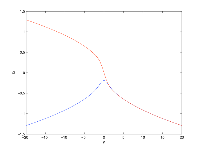
Figure 1: Real (blue) and imaginary part (red) of the tritronquée solution to the Painlevé I equation for $\zeta=iy$.

The values of $\Omega$ in between the collocation points are obtained by interpolation via the cubic polynomials in terms of which the solution has been constructed. This interpolation leads to a loss in accuracy of roughly one order of magnitude with respect to the precision at the collocation points. To test this we determine the numerical solution via bvp4c for P-I on Chebychev collocation points and check the accuracy with which the equation is satisfied via Chebychev differentiation, see e.g. [45]. It is found that the numerical solution with a relative tolerance of $10^{-10}$ on the collocation points satisfies the ODE to roughly the same order except at the boundary points where it is of the order $10^{-8}$, see Fig. 2 where we show the residual $\Delta$ by plugging the numerical solution into the differential equation for the above example. It is straightforward to achieve a prescribed accuracy by requiring a certain value for the relative tolerance. Notice that we are not interested in a high precision solution of P-I here, but in a comparison of solutions to the NLS equation close to the point of gradient catastrophe of the semiclassical system with an asymptotic solution in terms of P-I transcendents. For this purpose an accuracy of the solution of the order of $10^{-4}$ will be sufficient in all studied cases.

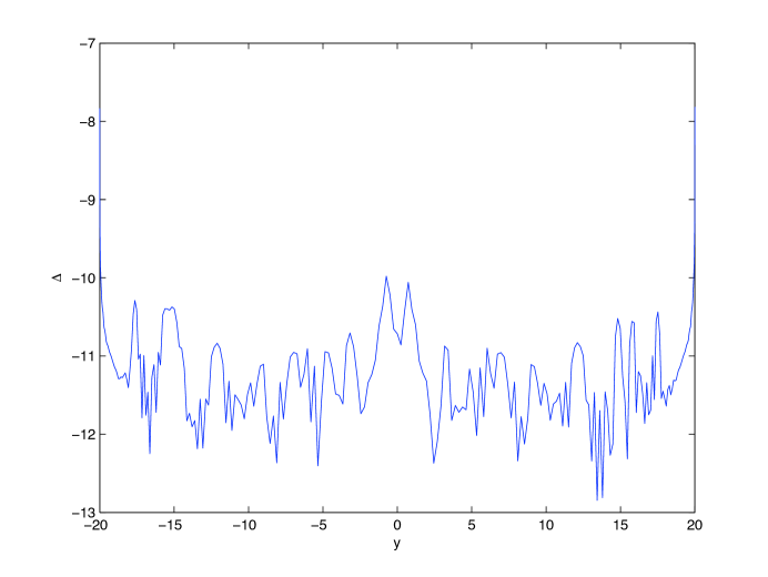
Figure 2: Error in the solution of the Painlevé I equation.

The quality of the used boundary conditions via the asymptotic behavior can be checked by computing the solution for different values of $y_{0}$. One finds that the difference between the asymptotic square root and the tritronquée solution is only visible near the origin, see Fig. 3. For large $x$ it can be seen that the difference between the square root asymptotics and the tritronquée solution reaches quickly values below the aimed at threshold of $10^{-4}$. It is interesting to note that this difference is actually smaller than the difference between the tritronquée solution and the truncated formal asymptotic series except at the boundary, where the latter condition is implemented (see Fig. 3).

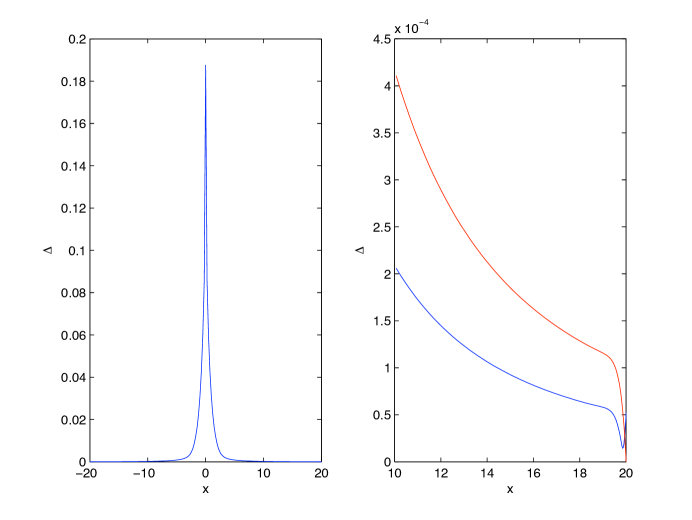
Figure 3: The plot on the left side shows the absolute value of the difference between the tritronquée solution and the asymptotic condition $-\sqrt{\zeta/6}$ for $a=i$ and $b=0$. The plot on the right side shows in blue the same difference for $x>10$ and in red the difference between the tritronquée solution and the truncated asymptotic series.

The dominant behavior of the square root changes if one approaches the critical lines $a=\exp(4\pi i/5)$, $b=0$. As can be seen from Fig. 4, the solution shows oscillations on top of the square root. The closer one comes to the critical lines, the slower is the fall off of the amplitude of the oscillations. We conjecture that these oscillations will have on the critical lines only a slow algebraic fall off towards infinity.

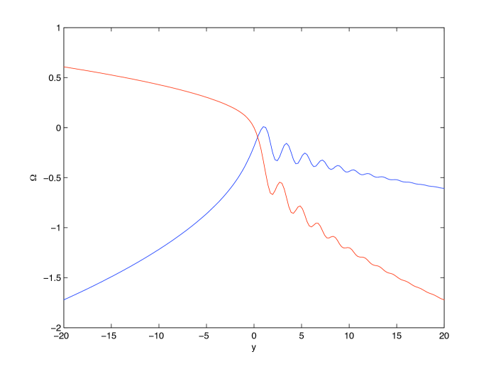
Figure 4: Real (blue) and imaginary part (red) of the tritronquée solution close to the critical line (for $a=\exp(i(4\pi/5-.05))$) with oscillations of slowly decreasing amplitude.

The above approach thus allows the computation of the tritronquée solution for a line avoiding the sector $|\arg\zeta|>4\pi/5$ with high accuracy. The picture one obtains by computing $\Omega$ along several such lines is that there are indeed no singularities in the sector $|\arg\zeta|<4\pi/5$, and that the square root behavior is followed for large $|\zeta|$. To obtain a more complete picture, we compute the tritronquée solution for $|\arg\zeta|<4\pi/5-0.05$ and $|\zeta|<R$ ( we choose $R=20$). The boundary data for $|\zeta|=R$ follow as before from the truncated asymptotic series, the data for $\arg\,\zeta=\pm 4\pi/5-0.05$ are obtained by computing the tritronquée solution on the respective lines as above.

To solve the resulting boundary value problem for the P-I equation is, however, computationally expensive since we have to solve an equation in 2 real dimensions iteratively. Since the solution we want to construct is holomorphic there, we can instead solve the harmonicity condition (the two dimensional Laplace equation) for the given boundary conditions. To this end we introduce polar coordinates $r$, $\phi$ and use a spectral grid as described in [45]: the main point is a doubling of the interval $r\in[0,R]$ to $[-R,R]$ to allow for a better distribution of the Chebychev collocation points. Since we work with values of $\phi<\phi_{0}$, we cannot use the usual Fourier series approach for the azimuthal coordinate. Instead we use again a Chebychev collocation method. The found solution in the considered domain is shown in Fig. 5 and Fig. 6.

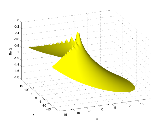
Figure 5: Real part of the tritronquée solution in the sector $r<20$ and $|\phi|<4\pi/5-0.05$.

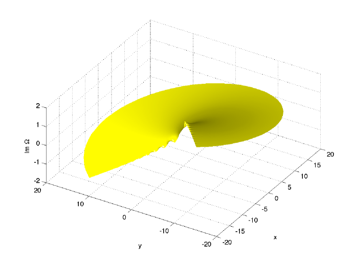
Figure 6: Imaginary part of the tritronquée solution in the sector $r<20$ and $|\phi|<4\pi/5-0.05$.

The quality of the solution can be tested by plugging the found solution to the Laplace equation into the P-I equation. Due to the low resolution and problems at the boundary, the accuracy is considerably lower in the two dimensional case than on the lines. This is, however, not a problem since we need only the one dimensional solutions for quantitative comparisons with NLS solutions. The two dimensional solutions give nonetheless strong numerical evidence for the conjecture that the tritronquée solution has globally no poles in the sector $|\arg\zeta|<4\pi/5$.

7 Critical behavior in NLS and the tritronquée solution of P-I: numerical results

In this section we will compare the numerical solution of the focusing NLS equation for two examples of initial data for values of $\epsilon$ between $0.1$ and $0.025$ with the asymptotic solutions discussed in the previous sections, the semiclassical solution up to the breakup and the tritronquée solution to the Painlevé I equation. The numerical approach to solve the NLS equation is discussed in detail in [29]. For values of $\epsilon$ below $0.04$ we have to use Krasny filtering [30] (Fourier coefficients with an absolute value below $10^{-13}$ are put equal to zero to avoid the excitation of unstable modes). With double precision arithmetic we could thus reach $\epsilon=0.025$, but could not go below.

7.1 Initial data

We consider initial data where $u(x,0)$ has a single positive hump, and where $v(x,0)$ is monotonously decreasing. For initial data of the form $u(x,0)=A^{2}(x)$ and $v(x,0)=0$ where the function $A(x)$ is analytic with a single positive hump with maximum value $A_{0}$, the semiclassical solution of NLS follows from (2.11) with $f(u,v)$ given by

$$f(u,v)=2\Im\left(\int\limits^{-\frac{1}{2}v+i\sqrt{u}}_{iA_{0}}d\eta\,\rho(\eta)\sqrt{(\eta+\frac{1}{2}v)^{2}+u}\right)$$ (7.1)

where

$$\rho(\eta)=\dfrac{\eta}{\pi}\int_{x^{-}(\eta)}^{x^{+}(\eta)}\dfrac{dx}{\sqrt{A^{2}(x)+\eta^{2}}},$$

and where $x^{\pm}(\eta)$ are defined by $A(x^{\pm}(\eta))=i\eta$. The formula (7.1) follows from results by S.Kamvissis, K.McLaughlin and P.Miller in [26].

From $f(u,v)$ it is straightforward to recover the initial data from the equations

$$x=f_{u},\quad f_{v}=0.$$ (7.2)

Numerically we study the critical behavior of two classes of initial data, one symmetric with respect to $x$ which were used in [34], and initial data without symmetry with respect to $x$ which are built from the initial data studied in [43]. For the former class the corresponding exact solution of focusing NLS is known in terms of a determinant. Nonetheless we integrate the NLS equation for these initial data numerically since this approach is not limited to special cases, but can be used for general smooth Schwartzian initial data as in the latter case.

7.1.1 Symmetric initial data

We consider the particular class of initial data data

$$u(x,t=0)=A_{0}^{2}\text{sech}^{2}\,x,\quad v(x,t=0)=-\mu\,\text{tanh}\,x,\quad\mu\geq 0.$$ (7.3)

Introducing the quantity

$$M=\sqrt{\frac{\mu^{2}}{4}-A_{0}^{2}},$$

we find that the semiclassical solution for these initial data follows from (2.11) with

$$\begin{split}f(u,v)=&\dfrac{\mu}{2}v-\dfrac{1}{4}(v-2M)\Delta_{+}-\dfrac{1}{4}(v+2M)\Delta_{-}-\dfrac{1}{2}u\log u\\ &+\dfrac{1}{2}u\log\left[(-\frac{1}{2}v+M+\Delta_{+})(-\frac{1}{2}v-M+\Delta_{-})\right]\end{split}$$ (7.4)

where

$$\Delta_{\pm}=\left((-\dfrac{1}{2}v\pm M)^{2}+u\right)^{\frac{1}{2}}.$$

For $\mu=0$ we recover the Satsuma-Yajima [37] initial data that were studied numerically in [34]. The function $f(u,v)$ takes the form

$$f(u,v)=\Re\left[\left(-\frac{v}{2}+i\,A_{0}\right)\sqrt{u+\left(-\frac{v}{2}+i\,A_{0}\right)^{2}}+u\,\log\frac{(-\frac{v}{2}+i\,A_{0})^{2}+\sqrt{(-\frac{v}{2}+iA_{0})^{2}+u}}{\sqrt{u}}\right],$$ (7.5)

which can also be recovered from (7.1) by setting $\rho=i$. The critical point is given by

$$u_{0}=2A_{0}^{2},\quad v_{0}=0,\quad x_{0}=0,\quad t_{0}=\frac{1}{2A_{0}}.$$ (7.6)

Furthermore we have

$$f_{uuu}^{0}=0,\quad f_{uuv}^{0}=\frac{1}{4A_{0}^{3}},\quad r=4A_{0}^{3},\quad\psi=0,$$ (7.7)

where $r$, $\psi$ are defined in (2.13). For $A_{0}=1$ the initial data (7.3) coincides with the one studied in [43] by A.Tovbis, S.Venakides and X.Zhou. In the particular case $\mu=2$, $A_{0}=1$ the function $f(u,v)$ in (7.1) simplifies to

$$f(u,v)=v-\frac{v}{2}\,\sqrt{\frac{1}{4}v^{2}+u}+u\log\left[\dfrac{-\frac{1}{2}v+\sqrt{\frac{1}{4}v^{2}+u}}{\sqrt{u}}\right].$$ (7.8)

In this case the critical point is given by

$$v_{0}=0,\;\;u_{0}=2+\mu,\quad t_{0}=\dfrac{1}{2+\mu},\;\;x_{0}=0.$$

Furthermore,

$$f_{uuu}^{0}=0,\quad f_{uuv}^{0}=\dfrac{2}{(\mu+2)^{3}},\quad r=\dfrac{(\mu+2)^{3}}{2},\quad\psi=0.$$

7.1.2 Non-symmetric initial data

Recall that we are interested here in Cauchy data in the Schwartz class of rapidly decreasing functions. The above initial data are symmetric with respect to $x$, $u$ is an even and $v$ an odd function in $x$. To obtain a situation which is manifestly not symmetric, we use the fact that if $f$ is a solution to (2.5), the same holds for derivatives and anti-derivatives of $f$ with respect to $v$ and for any linear combination of those. If $f_{v}$ is an even function in $v$, this will obviously not be the case for a linear combination of $f$ and $f_{v}$.

As a specific example, we consider the linear combination

$$f=f_{1}+\alpha f_{2},\quad\alpha=const,$$

where $f_{1}$ coincides with (7.8) and

$$f_{2}=2\,u\,\sqrt{\frac{1}{4}v^{2}+u}-\frac{2}{3}\left(\frac{1}{4}v^{2}+u\right)^{3/2}+u\,v\log\left[\dfrac{-\frac{1}{2}v+\sqrt{\frac{1}{4}v^{2}+u}}{\sqrt{u}}\right].$$ (7.9)

The function $f_{2}$ is obtained from the integration $f_{2,v}=f_{1}-v$. The critical point is given in this case by

$$u_{0}=4(1-16\alpha^{2}),\quad v_{0}=-16\alpha,\quad x_{0}=\frac{1}{2}\log\frac{1+4\alpha}{1-4\alpha},\quad t_{0}=\frac{1}{4}-\frac{\alpha}{2}\log\frac{1+4\alpha}{1-4\alpha};$$

thus we have $|\alpha|<1/4$. Furthermore,

$$f_{uuv}^{0}=-\frac{4\alpha^{2}-1/8}{4\sqrt{1-16\alpha^{2}}},\quad f_{uuu}^{0}=\frac{\alpha}{4\sqrt{1-16\alpha^{2}}},$$

such that

$$r=8u_{0},\quad\psi=-\arctan\dfrac{\alpha\sqrt{1-16\alpha^{2}}}{1/8-4\alpha^{2}}.$$

We determine the initial data corresponding to $f$ for a given value of $|\alpha|<1/4$ by solving (7.2) for $u$, $v$ in dependence of $x$. This is done numerically by using the algorithm of [31] which is implemented as the function fminsearch in Matlab. The algorithm provides an iterative approach which converges in our case rapidly if the starting values are close enough to the solution, which is achieved by choosing $u$ and $v$ corresponding to $f_{0}$ as an initial guess. For $\alpha$ close to $1/4$ we observe numerically a steepening of the initial pulse which will lead to a shock front in the limit $\alpha\to 1/4$. For the computations presented here, we consider the case $\alpha=0.1$ which leads to the initial data shown in Fig. 7.

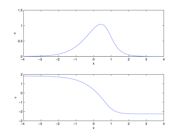
Figure 7: Initial data for the NLS equations without symmetry with respect to $x$.

The initial data are computed in the way described above to the order of the Krasny filter on the interval $x\in[-15,11]$ on Chebychev collocation points. Standard interpolation via Chebychev polynomials is then used to interpolate the resulting data to a Fourier grid. To avoid a Gibbs phenomenon at the interval ends due to the non-periodicity of the data, we use a Fourier grid on the interval $[-10\pi,10\pi]$ to ensure that the function $u$ takes values of the order of the Krasny filter. For $x<-15$ and $x>11$, the function $u$ is exponentially small which implies the zero-finding algorithm will no longer provide the needed precision. Thus we determine the exponential tails of the solution to leading order analytically. We find for $x\to-\infty$

$$u =v_{+}^{2}\exp\left(\frac{2(x-\alpha v_{+})}{\alpha v_{+}+1}\right),$$

$$v =v_{+}-v_{+}\exp\left(\frac{2(x-\alpha v_{+})}{\alpha v_{+}+1}\right)\left(2\log(v_{+})+\frac{2(x-\alpha v_{+})}{\alpha v_{+}+1}\right),$$ (7.10)

and for $x\to+\infty$

$$u =v_{-}^{2}\exp\left(-\frac{2(x+\alpha)}{\alpha v_{-}+1}\right)$$

$$v =v_{-}-v_{-}\exp\left(-\frac{2(x+\alpha)}{\alpha v_{-}+1}\right)\left(2\log(-v_{-})-\frac{2(x+\alpha)}{\alpha v_{-}+1}\right),$$ (7.11)

where $v_{\pm}=(\sqrt{1\pm\alpha}-1)/\alpha$. The initial data for the NLS equation in the form $\Psi=\sqrt{u}\exp(iS/\epsilon)$ are then found by integrating $v$ on the Chebychev grid by standard integration of Chebychev polynomials. The exponential tails for $S$ follow from (7.10) and (7.11). The matching of the tails to the Chebychev interpolant is not smooth and leads to a small Gibbs phenomenon. The Fourier coefficients decrease, however, to the order of the Krasny filter which is sufficient for our purposes. Thus we obtain the non-symmetric initial data with roughly the same precision as the analytic symmetric data.

7.2 Semiclassical solution

For times $t\ll t_{c}$, the semiclassical solution gives a very accurate asymptotic description for the NLS solution. The situation is similar to the Hopf and the KdV equation [19]. We find for the symmetric initial data for $t=t_{c}/2$ that the $L_{\infty}$ norm of the difference between the solutions decreases as $\epsilon^{2}$. More precisely a linear regression analysis in the case of symmetric initial data (for the values $\epsilon=0.03,0.04,\ldots,0.1$) for the logarithm of this norm leads to an error proportional to $\epsilon^{a}$ with $a=1.94$, a correlation coefficient $r=0.9995$ and standard error $\sigma_{a}=0.03$. In the non-symmetric case, we find $a=1.98$, $r=0.999996$ and $\sigma_{a}=0.003$.

Close to the critical time the semiclassical solution only provides a satisfactory description of the NLS solution for large values of $|x-x_{c}|$. In the breakup region it fails to be accurate since it develops a cusp at $x_{c}$ whereas the NLS solution stays smooth. This behavior can be well seen in Fig. 8 for the symmetric initial data.

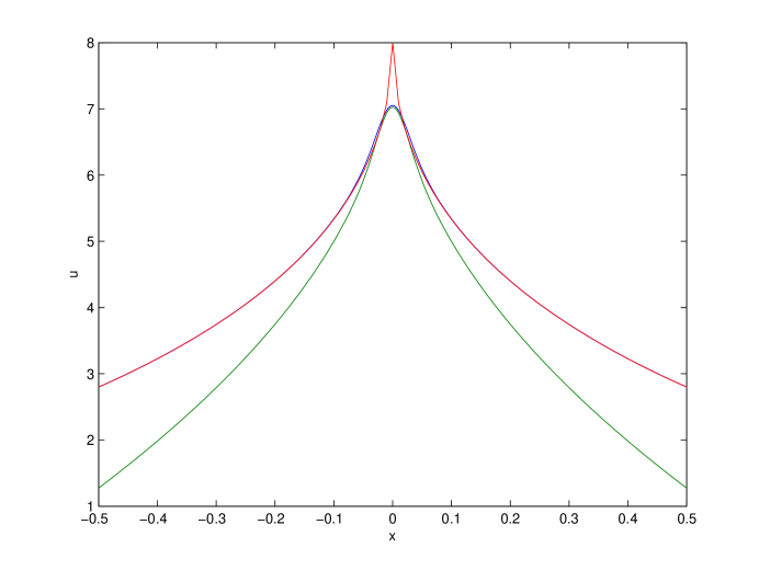
Figure 8: The blue line is the function $u$ of the solution to the focusing NLS equation for the initial data $u(x,0)=2\,\mbox{sech}\,x$ and $\epsilon=0.04$ at the critical time, and the red line is the corresponding semiclassical solution given by formulas (2.4). The green line gives the multiscales solution via the tritronquée solution of the Painlevé I equation.

The largest difference between the semiclassical and the NLS solution is always at the critical point. We find that the $L_{\infty}$ norm of the difference scales roughly as $\epsilon^{2/5}$ as suggested by the Main Conjecture. More precisely we find a scaling proportional to $\epsilon^{a}$ with $a=0.38$ and $r=0.999997$ and $\sigma_{a}=4.2*10^{-4}$. For the non-symmetric initial data, we find $a=0.36$, $r=0.9999$ and $\sigma_{a}=0.002$. The corresponding plot for $u$ can be seen in Fig. 9.

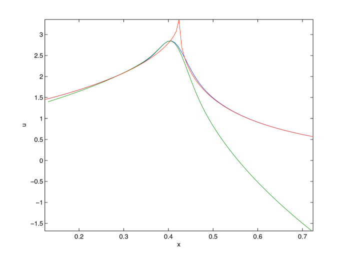
Figure 9: The blue line is the function $u$ of the solution to the focusing NLS equation for the non-symmetric initial data and $\epsilon=0.04$ at the critical time, and the red line is the corresponding semiclassical solution given by formulas (2.4). The green line gives the multiscales solution via the tritronquée solution of the Painlevé I equation.

The function $v$ for the same situation as in Fig. 8 is shown in Fig. 10. It can be seen that the semiclassical solution is again a satisfactory description for $|x-x_{c}|$ large, but fails to be accurate close to the breakup point.

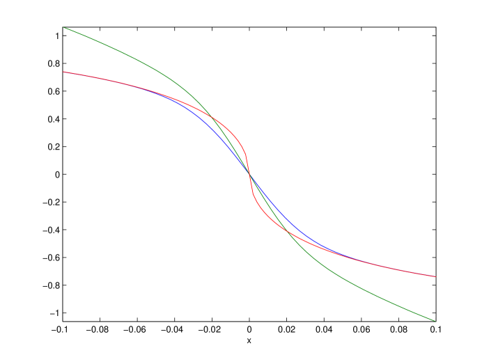
Figure 10: The blue line is the function $v$ of the solution to the focusing NLS equation for the initial data $u_{0}(x)=2\,\mbox{sech}\,x$ and $\epsilon=0.04$ at the critical time, and the red line is the corresponding semiclassical solution given by formulas (2.4). The green line gives the multiscales solution via the tritronquée solution of the Painlevé I equation.

The phase for the non-symmetric initial data can be seen in Fig. 11.

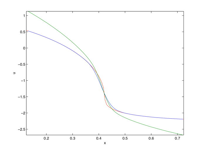
Figure 11: The blue line is the function $v$ of the solution to the focusing NLS equation for the non-symmetric initial data and $\epsilon=0.04$ at the critical time, and the red line is the corresponding semiclassical solution given by formulas (2.4). The green line gives the multiscales solution via the tritronquée solution of the Painlevé I equation.

In the following we will always study the scaling for the function $u$ without further notice.

7.3 Multiscales solution

It can be seen in Fig. 8 and Fig. 10 that the multiscales solution (5) in terms of the tritronquée solution to the Painlevé I equation gives a much better asymptotic description to the NLS solution at breakup close to the breakup point than the semiclassical solution for the symmetric initial data. For larger values of $|x-x_{c}|$, the semiclassical solution provides, however, the better approximation. The rescaling of the coordinates in (5) suggests to consider the difference between the NLS and the multiscales solution in an interval $[-\gamma\epsilon^{4/5},\gamma\epsilon^{4/5}]$ (we choose here $\gamma=1$, but within numerical accuracy the result does not depend on varying $\gamma$ around this value). These intervals can be seen in Fig. 12. We find that the $L_{\infty}$ norm of the difference between these solutions in this interval scales roughly like $\epsilon^{4/5}$. More precisely we have a scaling $\epsilon^{a}$ with $a=0.76$ ($r=0.998$ and $\sigma_{a}=0.019$).

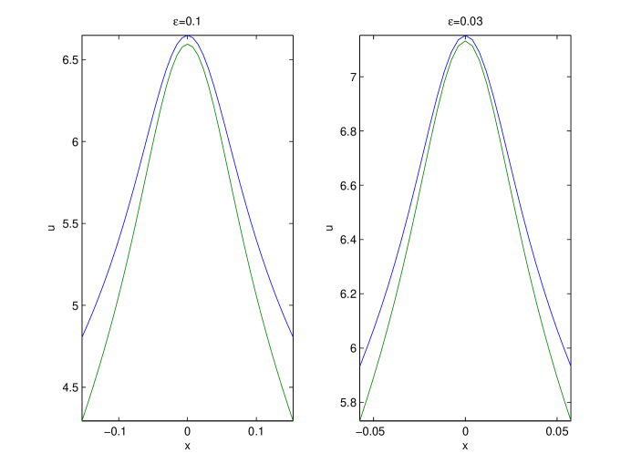
Figure 12: The blue line is the solution to the focusing NLS equation for the initial data $u_{0}(x)=2\,\mbox{sech}\,x$ at the critical time, and the green line gives the multiscales solution via the tritronquée solution of the Painlevé I equation. The plots are shown for two values of $\epsilon$ at the critical time.

For the non-symmetric initial data, the situation at the critical point can be seen in Fig. 9 and Fig. 11. Again the multiscales solution (5) gives a much better description close to the critical point than the semiclassical solution. However, the approximation is here much better on the side with weak slope for $u$ than on the side with strong slope. We consider again the $L_{\infty}$-norm of the difference between the multiscales and the NLS solution in the interval $[-\gamma\epsilon^{4/5},\gamma\epsilon^{4/5}]$. The scaling behavior of the solution can be seen in Fig. 13. For $\gamma=1$ we find $a=0.71$, $r=0.998$ and $\sigma_{a}=0.02$. These values do not change much for larger $\gamma$. For smaller $\gamma$ there are not enough points to provide a valid statistics. The value of $a$ smaller than the predicted $4/5$ is seemingly due to the strong asymmetry in the quality of the approximation of NLS by the multiscales solution as can be seen from Fig. 9. In the considered interval, the deviation is already so big that the scaling no longer holds as in the symmetric case. To study the scaling with a reliable statistics would, however, require the use of a considerably higher resolution which would be computationally too expensive.

Figure 13: The blue line is the solution to the focusing NLS equation for the non-symmetric initial data at the critical time, and the green line gives the multiscales solution via the tritronquée solution of the Painlevé I equation. The plots are shown for two values of $\epsilon$ at the critical time.

Going beyond the critical time, one finds that the real part of the NLS solution continues to grow before the central hump breaks up into several humps. Notice that the multiscales solution always leads to a function $u$ that is smaller than the corresponding function of the NLS solution at breakup and before. This changes for times after the breakup as can be inferred from Fig. 14 which shows the time dependence of the NLS and the corresponding multiscales solution for the non-symmetric initial data. The approximation is always best at the critical time.

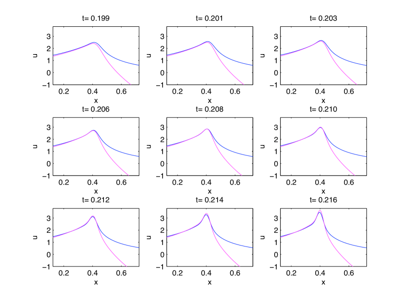
Figure 14: The blue line is the solution to the focusing NLS equation for the non-symmetric initial data for $\epsilon=0.04$ for various times, and the magenta line gives the multiscales solution via the tritronquée solution of the Painlevé I equation. The plot in the middle shows the behavior at the critical time.

To study the quality of the approximation (5), we use rescaled times. The scaling of the coordinates in (5) suggests to consider the NLS solution close to breakup at the times $t_{\pm}(\epsilon)$ with

$$t_{\pm}(\epsilon)=t_{c}+u_{0}/r-\sqrt{(u_{0}/r)^{2}\pm\epsilon^{4/5}\beta},$$ (7.12)

where $\beta$ is a constant (we consider $\beta=0.1$). We will only study the symmetric initial data in this context. Before breakup we obtain the situation shown in Fig. 15. It can be seen that the multiscales solution always provides a better description close to $x_{c}$ than the semiclassical solution, and that the quality improves in this respect with decreasing $\epsilon$. We find that the $L_{\infty}$ norm of the difference scales in this case as $\epsilon^{a}$ with $a=0.55$ ($r=0.994$ and $\sigma_{a}=0.03$).

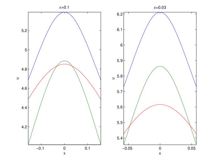
Figure 15: The blue line is the solution to the focusing NLS equation for the initial data $u_{0}(x)=2\,\mbox{sech}\,x$, and the red line is the corresponding semiclassical solution given by formulas (2.4). The green line gives the multiscales solution via the tritronquée solution of the Painlevé I equation. The plots are shown for two values of $\epsilon$ at the corresponding times $t_{-}(\epsilon)$.

The situation for times after breakup can be inferred from Fig. 16. Close to the central region the multiscales solution shows a clear difference to the NLS solution. But it is interesting to note that the ripples next to the central hump are well approximated by the Painlevé I solution. The $L_{\infty}$ norm of the difference between the two solutions scales roughly like $\epsilon$. More precisely we find a scaling $\epsilon^{a}$ with $a=1.02$ ($r=0.9999$ and $\sigma_{a}=7.7*10^{-3}$).

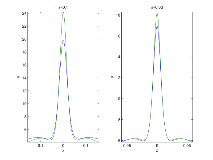
Figure 16: The blue line is the solution to the focusing NLS equation for the initial data $u_{0}(x)=2\,\mbox{sech}\,x$, and the green line gives the multiscales solution via the tritronquée solution of the Painlevé I equation. The plots are shown for two values of $\epsilon$ at the corresponding times $t_{+}(\epsilon)$.

8 Concluding remarks

In this paper we have started the study of the critical behavior of generic solutions of the focusing nonlinear Schrödinger equation. We have formulated the conjectural analytic description of this behavior in terms of the tritronquée solution to the Painlevé-I equation restricted to certain lines in the complex plane. We provided analytical as well as numerical evidence supporting our conjecture. In subsequent publications we plan to further study the Main Conjecture of the present paper by applying techniques based, first of all, on the Riemann - Hilbert problem method [26, 43, 44] and the theory of Whitham equations (see [19] for the numerical implementation of the Whitham procedure in the analysis of oscillatory behavior of solutions to the KdV equations). The latter will also be applied to the asymptotic description of solutions inside the oscillatory zone. Furthermore we plan to study the possibility of extending the Main Conjecture to the critical behavior of solutions to the Hamiltonian perturbations of more general first order quasilinear systems of elliptic type. Last but not least, it would be of interest to study the distribution of poles of the tritronquée solution in the sector $|\arg\zeta|>\frac{4\pi}{5}$ and to compare these poles with the peaks of solutions to NLS inside the oscillatory zone. The elliptic asymptotics obtained by Kitaev [28] might be useful for studying these poles for large $|\zeta|$.

In this paper we did not study the behaviour of solutions to NLS near the boundary $u=0$. Such a study is postponed for a subsequent publication.

References

- [1] G.P.Agrawal, Nonlinear Fiber Optics. Academic Press, San Diego, 2006, 4th edition.
- [2] S.Alinhac, Blowup for Nonlinear Hyperbolic Equations. Progress in Nonlinear Differential Equations and their Applications, 17. Birkhäuser Boston, Inc., Boston, MA, 1995.
- [3] V.I.Arnold,V.V.Goryunov, O.V.Lyashko,V.A.Vasil’ev, Singularity Theory. I. Dynamical systems. VI, Encyclopaedia Math. Sci. 6, Springer, Berlin, 1993.
- [4] P.Boutroux, Recherches sur les transcendants de M. Painlevé et l’étude asymptotique des équations différentielles du second ordre. Ann. École Norm 30 (1913) 265 - 375.
- [5] J.C.Bronski, J.N.Kutz, Numerical simulation of the semiclassical limit of the focusing nonlinear Schrödinger equation. Phys. Lett. A 254 (2002) 325 - 336.
- [6] R.Buckingham, S.Venakides, Long-time asymptotics of the nonlinear Schrödinger equation shock problem. Comm. Pure Appl. Math., Published Online 12.03.2007.
- [7] R.Carles, WKB analysis for the nonlinear Schrödinger equation and instability results. ArXiv:math.AP/0702318.
- [8] H.D.Ceniceros, F.-R.Tian, A numerical study of the semi-classical limit of the focusing nonlinear Schrödinger equation. Phys. Lett. A 306 (2002) 25–34.
- [9] T.Claeys, M.Vanlessen, The existence of a real pole-free solution of the fourth order analogue of the Painlevé I equation. ArXiv:math-ph/0604046.
- [10] O.Costin, Correlation between pole location and asymptotic behavior for Painlevé I solutions. Comm. Pure Appl. Math. 52 (1999) 461–478.
- [11] M.C.Cross and P.C.Hohenberg, Pattern formation outside of equilibrium. Rev. Mod. Phys. 65 (1993) 851-1112.
- [12] B.Dubrovin, S.-Q.Liu, Y.Zhang, On Hamiltonian perturbations of hyperbolic systems of conservation laws I: quasitriviality of bihamiltonian perturbations. Comm. Pure Appl. Math. 59 (2006) 559-615.
- [13] B.Dubrovin, On Hamiltonian perturbations of hyperbolic systems of conservation laws, II: universality of critical behaviour, Comm. Math. Phys. 267 (2006) 117 - 139.
- [14] M.Duits, A.Kuijlaars, Painlevé I asymptotics for orthogonal polynomials with respect to a varying quartic weight. ArXiv:math/0605201.
- [15] A.S.Fokas, S.Tanveer, A Hele - Shaw problem and the second Painlevé transcendent. Math. Proc. Camb. Phil. Soc. 124 (1998) 169 - 191.
- [16] M.G.Forest, J.E.Lee, Geometry and modulation theory for the periodic nonlinear Schrödinger equation. In: Oscillation Theory, Computation, and Methods of Compensated Compactness (Minneapolis, Minn., 1985), 35-69. The IMA Volumes in Mathematics and Its Applications, 2. Springer, New York, 1986.
- [17] J. Ginibre, G.Velo, On a class of nonlinear Schrödinger equations. I. The Cauchy problem, general case. J. Funct. Anal. 32 (1979) 1-32.
- [18] I. S.Gradshteyn, I. M. Ryzhik, Table of Integrals, Series, and Products. Translated from the Russian. Sixth edition. Translation edited and with a preface by Alan Jeffrey and Daniel Zwillinger. Academic Press, Inc., San Diego, CA, 2000.
- [19] T.Grava, C.Klein, Numerical solution of the small dispersion limit of Korteweg de Vries and Whitham equations. ArXiv:math-ph0511011, to appear in Comm. Pure Appl. Math., 2007.
- [20] T.Grava, C.Klein, Numerical study of a multiscale expansion of KdV and Camassa-Holm equation. ArXiv:math-ph/0702038.
- [21] E.Grenier, Semiclassical limit of the nonlinear Schrödinger equation in small time. Proc. Amer. Math. Soc. 126 (1998) 523–530.
- [22] E.L.Ince, Ordinary Differential Equations. Dover Publications, New York, 1944.
- [23] S.Jin, C.D.Levermore, D.W.McLaughlin, The behavior of solutions of the NLS equation in the semiclassical limit. Singular Limits of Dispersive Waves (Lyon, 1991), 235–255, NATO Adv. Sci. Inst. Ser. B Phys., 320, Plenum, New York, 1994.
- [24] N.Joshi, A.Kitaev, On Boutroux’s tritronquée solutions of the first Painlevé equation. Stud. Appl. Math. 107 (2001) 253–291.
- [25] S.Kamvissis, Long time behavior for the focusing nonlinear Schrödinger equation with real spectral singularities. Comm. Math. Phys. 180 (1996) 325–341.
- [26] S. Kamvissis, K.D.T.-R.McLaughlin, P.D.Miller, Semiclassical Soliton Ensembles for the Focusing Nonlinear Schrödinger Equation. Annals of Mathematics Studies, 154. Princeton University Press, Princeton, NJ, 2003.
- [27] A.Kapaev, Quasi-linear Stokes phenomenon for the Painlevé first equation. J. Phys. A: Math. Gen. 37 (2004) 11149–11167.
- [28] A.Kitaev, The isomonodromy technique and the elliptic asymptotics of the first Painlevé transcendent. Algebra i Analiz 5 (1993), no. 3, 179–211; translation in St. Petersburg Math. J. 5 (1994), no. 3, 577–605.
- [29] C. Klein, Fourth order time-stepping for low dispersion Korteweg - de Vries and nonlinear Schrödinger equation (2006), http://www.mis.mpg.de/preprints/2006/prepr133.html
- [30] R.Krasny, A study of singularity formation in a vortex sheet by the point-vortex approximation. J. Fluid Mech. 167 (1986) 65–93.
- [31] J. C. Lagarias, J. A. Reeds, M. H. Wright, and P. E. Wright, Convergence properties of the Nelder-Mead simplex method in low dimensions. SIAM Journal of Optimization 9 (1988) 112-147.
- [32] G.D.Lyng, P.D.Miller, The -soliton of the focusing nonlinear Schrödinger equation for large. Comm. Pure Appl. Math. 60 (2007) 951-1026.
- [33] G.Métivier, Remarks on the well-posedness of the nonlinear Cauchy problem. ArXiv:math.AP/0611441.
- [34] P.D.Miller, S.Kamvissis, On the semiclassical limit of the focusing nonlinear Schrödinger equation. Phys. Lett. A 247 (1998) 75–86.
- [35] A.C.Newell, Solitons in Mathematics and Physics. CBMS-NSF Regional Conference Series in Applied Mathematics, 48. SIAM, Philadelphia, PA, 1985.
- [36] S.P.Novikov, S.V.Manakov, L.P.Pitaevskiĭ, V.E.Zakharov, Theory of Solitons. The Inverse Scattering Method. Translated from the Russian. Contemporary Soviet Mathematics. Consultants Bureau [Plenum], New York, 1984.
- [37] J. Satsuma and N. Yajima, Initial value problems of one-dimensional self-modulation of nonlinear waves in dispersive media, Supp. Prog. Theo. Phys. 55 (1974), pp. 284 -306.
- [38] A.B.Shabat, One-dimensional perturbations of a differential operator, and the inverse scattering problem. In: Problems in Mechanics and Mathematical Physics, 279–296. Nauka, Moscow, 1976.
- [39] L. F. Shampine, M. W. Reichelt and J. Kierzenka, Solving Boundary Value Problems for Ordinary Differential Equations in MATLAB with bvp4c, available at http://www.mathworks.com/bvp_tutorial
- [40] P.Sikivie, The caustic ring singularity. Phys. Rev. D60 (1999) 063501.
- [41] M.Slemrod, Monotone increasing solutions of the Painlevé 1 equation and their role in the stability of the plasma-sheath transition. European J. Appl. Math. 13 (2002) 663–680.
- [42] R.Thom, Structural Stability and Morphogenesis: An Outline of a General Theory of Models. Reading, MA: Addison-Wesley, 1989.
- [43] A.Tovbis, S.Venakides, X.Zhou, On semiclassical (zero dispersion limit) solutions of the focusing nonlinear Schrödinger equation. Comm. Pure Appl. Math. 57 (2004) 877–985.
- [44] A.Tovbis, S.Venakides, X.Zhou, On the long-time limit of semiclassical (zero dispersion limit) solutions of the focusing nonlinear Schödinger equation: pure radiation case. Comm. Pure Appl. Math. 59 (2006) 1379–1432.
- [45] L. N. Trefethen, Spectral Methods in MATLAB, SIAM, Philadelphia, PA, 2000.
- [46] Y.Tsutsumi, -solutions for nonlinear Schrödinger equations and nonlinear groups. Funkcial. Ekvac. 30 (1987) 115–125.
- [47] G.B.Whitham, Linear and Nonlinear Waves. Wiley-Intersci. 1974.
- [48] V.E.Zakharov, A.B.Shabat, A. B. Exact theory of two-dimensional self-focusing and one-dimensional self-modulation of waves in nonlinear media. Soviet Physics JETP 34 (1972), no. 1, 62-69.; translated from Ž. Eksper. Teoret. Fiz. (1971), no. 1, 118-134.