Optimal Shape Design for Stokes Flow
Via Minimax Differentiability

Abstract.  This paper is concerned with a shape sensitivity analysis of a viscous incompressible fluid driven by Stokes equations with nonhomogeneous boundary condition. The structure of shape gradient with respect to the shape of the variable domain for a given cost function is established by using the differentiability of a minimax formulation involving a Lagrangian functional combining with function space parametrization technique or function space embedding technique. We apply an gradient type algorithm to our problem. Numerical examples show that our theory is useful for practical purpose and the proposed algorithm is feasible.
Keywords.  shape optimization; minimax formulation; gradient algorithm; Stokes equations.
AMS(2000) subject classifications. 49J35, 49K35, 49K40, 35B37.

1 Introduction

This paper deals with the optimal shape design for Stokes flow inside a moving domain. This problem is a basic tool in the design and control of many industrial devices such as aircraft wings, automobile shapes, boats, and so on. The control variable is the shape of the domain, the object is to minimize a cost function that may be given by the designer, and finally we can obtain the optimal shapes.

The efficient computation of optimal shapes requires a shape calculus (see [7]) which differs from its analog in vector spaces. It is necessary to make sense of shape gradient which is a basic tool to obtain necessary conditions and to provide us with gradient information required by the gradient type optimization methods. The velocity method (see J.Cea[3] and J.-P.Zolesio[7, 18]) gave a precise mathematical meaning to this notion.

Many shape optimization problems can be expressed as a minimax of some suitable Lagrangian functional. The characterization of the change in geometric domain is obtained by velocity method. Finally the use of theorems on the differentiability of a saddle point (i.e., a minimax) of such lagrangian functional with respect to a parameter provides very powerful tools to obtain shape gradient by function space parametrization or function space embedding (see[5]) without the usual study of the derivative of the state.

The function space parametrization technique and function space embedding technique are advocated by M.C.Delfour and J.-P.Zolésio to solving poisson equation with Dirichlet and Nuemann condition (see[7]). In our paper [8], we apply them to a Robin problem and give its numerical implementation. The purpose of this paper is to use lagrangian formulation and theorem on the differentiability of a minimax to study the shape sensitivity analysis for Stokes flow, and then give a gradient type algorithm with some numerical examples to prove that our theory could be very useful for the practical purpose.

This paper is organized as follows. Section 2 is devoted to the statement of a shape optimization problem for Stokes flow. In section 3, we briefly recall the velocity method which is used for the characterization of the deformation of the shape of the domain, and we also give the definitions of Eulerian derivative and shape gradient. Then we include the divergence free condition directly into the Lagrange functional thanks to a multiplier which plays the role of the adjoint state associated with the primal pressure. This leads to a saddle point formulation of the shape optimization problem for Stokes equations with nonhomogeneous boundary condition.

Section 4 is devoted to the computation of the shape gradient of the Lagrangian functional due to a minimax principle concerning the differentiability of the minimax formulation(see[4, 5]) by Function Space Parametrization technique.

In section 5, we compute the shape gradient by using such minimax principle coupling with Function Space Embedding technique and get the same expression obtained in section 4.

Finally, in the last section, with the shape gradient information, we can establish a gradient type algorithm to solve our problem, and numerical examples show the feasibility of our approach for different viscosity coefficients.

Before closing this section, we introduce some notations that will be used throughout the paper.

$H^{m}(D),m\in\mathbb{R},$ denotes the standard Sobolev space of order $m$ with respect to the set $D$, where $D$ is either the fluid domain $\Omega$ or its boundary $\Gamma$. Note that $H^{0}(D)=L^{2}(D)$. Corresponding Sobolev spaces of vector-valued functions will be denoted by $H^{m}(D)^{N}$.

Let $\mbox{\boldmath$u$}=(u_{1},u_{2},\cdots,u_{d})$ and $\mbox{\boldmath$v$}=(v_{1},v_{2},\cdots,v_{d})$ be two vector functions of dimension $d$, and $w$ be a scalar function. $\mathrm{D}\mbox{\boldmath$u$}$ denotes the Jacobian matrix of $u$, i.e., $\mathrm{D}\mbox{\boldmath$u$}{\,\stackrel{{\scriptstyle\mbox{\rm\tiny def}}}{{=}}\,}(\partial_{j}u_{i})_{i,j=1}^{d}$, and its transpose matrix is denoted by ${}^{*}\mathrm{D}\mbox{\boldmath$u$}$. We also have the following linear forms:

$$(\mbox{\boldmath$u$},\mbox{\boldmath$v$})_{\Omega}{\,\stackrel{{\scriptstyle\mbox{\rm\tiny def}}}{{=}}\,}\int_{\Omega}\mbox{\boldmath$u$}\cdot\mbox{\boldmath$v$}\,\mathrm{d}x=\int_{\Omega}\langle\mbox{\boldmath$u$},\mbox{\boldmath$v$}\rangle\,\mathrm{d}x=\int_{\Omega}\sum\limits^{d}_{i=1}u_{i}\,v_{i}\,\mathrm{d}x,\quad\forall\mbox{\boldmath$u$},\mbox{\boldmath$v$}\in L^{2}(\Omega)^{d};$$

$$a(\Omega;\mbox{\boldmath$u$},\mbox{\boldmath$v$}){\,\stackrel{{\scriptstyle\mbox{\rm\tiny def}}}{{=}}\,}\int_{\Omega}\alpha\,\mathrm{D}\mbox{\boldmath$u$}:\mathrm{D}\mbox{\boldmath$v$}\,\mathrm{d}x=\int_{\Omega}\alpha\sum\limits^{d}_{i,j=1}\partial_{j}u_{i}\,\partial_{j}v_{i}\,\mathrm{d}x,\quad\forall\mbox{\boldmath$u$},\mbox{\boldmath$v$}\in H^{1}(\Omega)^{d};$$

$$b(\Omega;\mbox{\boldmath$u$},w){\,\stackrel{{\scriptstyle\mbox{\rm\tiny def}}}{{=}}\,}-\int_{\Omega}\,\mathrm{div}\mbox{\boldmath$u$}\,w\,\mathrm{d}x=-\int_{\Omega}\sum\limits_{i=1}^{d}\partial_{i}u_{i}\,w\,\mathrm{d}x,\quad\forall\mbox{\boldmath$u$}\in H^{1}(\Omega)^{d},\;\forall w\in L^{2}(\Omega).$$

Note that the inner products in $L^{2}(\Omega)^{d}$ is denoted by $(\cdot,\cdot)_{\Omega}$, and the angle product $\langle\cdot,\cdot\rangle$ denotes the usual dot product of two vectors in this paper.

2 Formulation of the problem

Let $\Omega$ be the fluid domain in $\mathbb{R}^{N}$($N=2\;\mbox{or}\;3$), and the boundary $\Gamma{\,\stackrel{{\scriptstyle\mbox{\rm\tiny def}}}{{=}}\,}\partial\Omega$ be smooth. The fluid is described by its velocity $y$ and pressure $p$ satisfying the Stokes equations:

$$\left\{\begin{array}[]{ll}-\alpha\Delta\mbox{\boldmath$y$}+\nabla p=\mbox{\boldmath$f$}&\quad\mbox{in}\;\Omega\\ \,\mathrm{div}\mbox{\boldmath$y$}=0&\quad\mbox{in}\;\Omega\\ \mbox{\boldmath$y$}=\mbox{\boldmath$g$}&\quad\mbox{on}\;\Gamma\end{array}\right.$$ (2.1)

where $\alpha$ stands for the kinematic viscosity coefficient. Let $\mbox{\boldmath$f$}\in{H^{m}(\mathbb{R}^{N})}^{N},$ and $\mbox{\boldmath$g$}\in{H^{m+3/2}(\mathbb{R}^{N})}^{N}$ ($m\geq 0$ to be specified) be given satisfying the compatibility condition

$$\int_{\Gamma}\mbox{\boldmath$g$}\cdot\mbox{\boldmath$n$}\,\mathrm{d}s=0,$$ (2.2)

then we know that the solution $(\mbox{\boldmath$y$},p)$ belongs to $H^{1}(\Omega)^{N}\times L^{2}(\Omega)$ and even to $H^{m+2}(\Omega)^{N}\times H^{m+1}(\Omega)$ when $\Gamma$ is of class $C^{m+2}$ by the regularity theorem (see[9, 17]).

Our objective is to compute the first order ”derivative” of the cost function

$$J(\Omega)=\frac{1}{2}\int_{\Omega}\lvert\mbox{\boldmath$y$}(\Omega)-\mbox{\boldmath$y$}_{d}\rvert^{2}\,\mathrm{d}x$$ (2.3)

with respect to the variational domain $\Omega$. The target velocity $\mbox{\boldmath$y$}_{d}$ is fixed in ${H^{1}(\mathbb{R}^{N})}^{N}$ and given by the designer for some purposes.

3 The velocity method and a saddle point formulation

Domains $\Omega$ don’t belong to a vector space and this requires the development of shape calculus to make sense of a “derivative” or a “gradient”. To realize it, there are about three types of techniques: J.Hadamard[11]’s normal variation method, the perturbation of the identity method by J.Simon[16] and the velocity method(see J.Cea[3] and J.-P.Zolesio[7, 18]). We will use the velocity method which contains the others.

Let $\mbox{\boldmath$V$}\in\mathrm{E}^{k}:=C([0,\tau);\mathcal{D}^{k}(\mathbb{R}^{N},\mathbb{R}^{N}))$, where $\mathcal{D}^{k}(\mathbb{R}^{N},\mathbb{R}^{N})$ denotes the space of all $k-$times continuous differentiable functions with compact support contained in $\mathbb{R}^{N}$ and $\tau$ is a small positive real number. The velocity field

$$\mbox{\boldmath$V$}(t)(x)=\mbox{\boldmath$V$}(t,x),\qquad x\in\mathbb{R}^{N},\quad t\geq 0$$

belongs to $\mathcal{D}^{k}(\mathbb{R}^{N},\mathbb{R}^{N})$ for each $t$. It can generate transformations

$$T_{t}(\mbox{\boldmath$V$})X=x(t,X),\quad t\geq 0,\quad X\in\mathbb{R}^{N}$$

through the following dynamical system

$$\left\{\begin{array}[]{ll}\frac{\,\mathrm{d}x}{\,\mathrm{d}t}(t,X)=\mbox{\boldmath$V$}(t,x(t))\\[3.0pt] x(0,X)=X\end{array}\right.$$ (3.1)

with the initial value $X$ given. We denote the ”transformed domain” $T_{t}(\mbox{\boldmath$V$})(\Omega)$ by $\Omega_{t}(\mbox{\boldmath$V$})$ at $t\geq 0$.

Furthermore, for sufficiently small $t>0,$ the Jacobian $J_{t}$ is strictly positive:

$$J_{t}(x):=\det\lvert\mathrm{D}T_{t}(x)\rvert=\det\mathrm{D}T_{t}(x)>0,$$ (3.2)

where $\mathrm{D}T_{t}(x)$ denotes the Jacobian matrix of the transformation $T_{t}$ evaluated at a point $x\in\mathbb{R}^{N}$ associated with the velocity field $V$. We will also use the following notation: $\mathrm{D}T_{t}^{-1}(x)$ is the inverse of the matrix $\mathrm{D}T_{t}(x)$ , ${}^{*}\mathrm{D}T_{t}^{-1}(x)$ is the transpose of matrix $\mathrm{D}T_{t}^{-1}(x)$, and the Jacobian matrix of $T_{t}$ with respect to the boundary $\Gamma$ is denoted by $w_{t}=J_{t}\lvert{}^{*}\mathrm{D}T_{t}^{-1}\,\mbox{\boldmath$n$}\rvert$.

We now consider the solution $(\mbox{\boldmath$y$}_{t},p_{t})$ on $\Omega_{t}$ of the problem

$$\left\{\begin{array}[]{ll}-\alpha\Delta\mbox{\boldmath$y$}_{t}+\nabla p_{t}=\mbox{\boldmath$f$}&\mbox{in}\;\Omega_{t}\\ \,\mathrm{div}\mbox{\boldmath$y$}_{t}=0,&\mbox{in}\;\Omega_{t}\\ \mbox{\boldmath$y$}_{t}=\mbox{\boldmath$g$}&\mbox{on}\;\Gamma_{t}\;(\mbox{the boundary of}\;\Omega_{t})\end{array}\right.$$ (3.3)

and the associated cost function

$$J(\Omega_{t})=\frac{1}{2}\int_{\Omega_{t}}\lvert\mbox{\boldmath$y$}_{t}-\mbox{\boldmath$y$}_{d}\rvert^{2}\,\mathrm{d}x$$ (3.4)

We say that this functional has a Eulerian derivative at $\Omega$ in the direction $V$ if the limit

$$\lim_{t\searrow 0}\frac{J(\Omega_{t})-J(\Omega)}{t}{\,\stackrel{{\scriptstyle\mbox{\rm\tiny def}}}{{=}}\,}\,\mathrm{d}J(\Omega;\mbox{\boldmath$V$})$$

exists.

Furthermore, if the map

$$\mbox{\boldmath$V$}\mapsto\,\mathrm{d}J(\Omega;\mbox{\boldmath$V$}):\;\mathrm{E}^{k}\rightarrow\mathbb{R}$$

is linear and continuous, we say that $J$ is shape differentiable at $\Omega$. In the distributional sense we have

$$\,\mathrm{d}J(\Omega;\mbox{\boldmath$V$})=\langle\Im,\mbox{\boldmath$V$}\rangle_{\mathcal{D}^{k}(\mathbb{R}^{N},\mathbb{R}^{N})^{\prime}\times\mathcal{D}^{k}(\mathbb{R}^{N},\mathbb{R}^{N})}.$$ (3.5)

When $J$ has a Eulerian derivative, we say that $\Im$ is the shape gradient of $J$ at $\Omega$.

Now we shall describe how to build an appropriate Lagrangian functional that takes into account the divergence condition and the nonhomogeneous Dirichlet boundary condition.

Given $\mbox{\boldmath$f$}\in{H^{1}(\mathbb{R}^{N})}^{N}$ and $\mbox{\boldmath$g$}\in{H^{5/2}(\mathbb{R}^{N})}^{N}$, we introduce a Lagrange multiplier $\mu$ and a functional

$$L(\Omega,\mbox{\boldmath$y$},p,\mbox{\boldmath$v$},q,\mbox{\boldmath$\mu$})=\int_{\Omega}\langle\alpha\Delta\mbox{\boldmath$y$}-\nabla p+\mbox{\boldmath$f$},\mbox{\boldmath$v$}\rangle\,\mathrm{d}x+\int_{\Omega}\,\mathrm{div}\mbox{\boldmath$y$}q\,\mathrm{d}x+\int_{\Gamma}\langle\mbox{\boldmath$y$}-\mbox{\boldmath$g$},\mbox{\boldmath$\mu$}\rangle\,\mathrm{d}s$$ (3.6)

for $(\mbox{\boldmath$y$},p)\in Y(\Omega)\times Q(\Omega)$, $(\mbox{\boldmath$v$},q)\in P(\Omega)\times Q(\Omega)$, and $\mbox{\boldmath$\mu$}\in H^{-1/2}(\Gamma)^{N}$ with

$$Y(\Omega_{t}){\,\stackrel{{\scriptstyle\mbox{\rm\tiny def}}}{{=}}\,}H^{2}(\Omega_{t})^{N};\qquad P(\Omega_{t}){\,\stackrel{{\scriptstyle\mbox{\rm\tiny def}}}{{=}}\,}H^{2}(\Omega_{t})^{N}\cap H^{1}_{0}(\Omega_{t})^{N};\quad Q(\Omega_{t}){\,\stackrel{{\scriptstyle\mbox{\rm\tiny def}}}{{=}}\,}H^{1}(\Omega_{t}),$$

and $\Omega_{0}=\Omega$ as $t=0$.

Now we’re interested in the following saddle point problem

$$\inf_{(\mbox{\boldmath$y$},p)\in Y(\Omega)\times Q(\Omega)}\quad\sup_{(\mbox{\boldmath$v$},q,\mbox{\boldmath$\mu$})\in P(\Omega)\times Q(\Omega)\times H^{-1/2}(\Gamma)^{N}}\;L(\Omega,\mbox{\boldmath$y$},p,\mbox{\boldmath$v$},q,\mbox{\boldmath$\mu$})$$

The solution is characterized by the following:

$\bullet$  The state $(\mbox{\boldmath$y$},p)$ is the solution of problem

$$\left\{\begin{array}[]{ll}-\alpha\Delta\mbox{\boldmath$y$}+\nabla p=\mbox{\boldmath$f$}&\quad\mbox{in}\;\Omega\\ \,\mathrm{div}\mbox{\boldmath$y$}=0&\quad\mbox{in}\;\Omega\\ \mbox{\boldmath$y$}=\mbox{\boldmath$g$}&\quad\mbox{on}\;\Gamma\end{array}\right.$$ (3.7)

$\bullet$  The adjoint state $(\mbox{\boldmath$v$},q)$ is the solution of problem

$$\left\{\begin{array}[]{ll}-\alpha\Delta\mbox{\boldmath$v$}+\nabla q=0&\mbox{in}\;\Omega\\ \,\mathrm{div}\mbox{\boldmath$v$}=0&\mbox{in}\;\Omega\\ \mbox{\boldmath$v$}=0&\mbox{on}\;\Gamma;\end{array}\right.$$ (3.8)

$\bullet$  The multiplier satisfies: $\mbox{\boldmath$\mu$}=\alpha\mathrm{D}\mbox{\boldmath$v$}\,\mbox{\boldmath$n$}-q\,\mbox{\boldmath$n$},\;\mbox{on}\;\Gamma$.

Hence we obtain the following new functional,

$$L(\Omega,\mbox{\boldmath$y$},p,\mbox{\boldmath$v$},q)=\int_{\Omega}\langle\alpha\Delta\mbox{\boldmath$y$}-\nabla p+\mbox{\boldmath$f$},\mbox{\boldmath$v$}\rangle\,\mathrm{d}x+\int_{\Omega}\,\mathrm{div}\mbox{\boldmath$y$}q\,\mathrm{d}x+\int_{\Gamma}\langle\mbox{\boldmath$y$}-\mbox{\boldmath$g$},\alpha\mathrm{D}\mbox{\boldmath$v$}\,\mbox{\boldmath$n$}-q\,\mbox{\boldmath$n$}\rangle\,\mathrm{d}s.$$

To get rid of the boundary integral, the following identities are derived by Green formula,

$$\int_{\Gamma}\langle\mbox{\boldmath$y$}-\mbox{\boldmath$g$},\mathrm{D}\mbox{\boldmath$v$}\mbox{\boldmath$n$}\rangle\,\mathrm{d}s = \int_{\Omega}[\langle\mbox{\boldmath$y$}-\mbox{\boldmath$g$},\Delta\mbox{\boldmath$v$}\rangle+\mathrm{D}(\mbox{\boldmath$y$}-\mbox{\boldmath$g$}):\mathrm{D}\mbox{\boldmath$v$}]\,\mathrm{d}x;$$

$$\int_{\Gamma}\langle\mbox{\boldmath$y$}-\mbox{\boldmath$g$},q\,\mbox{\boldmath$n$}\rangle\,\mathrm{d}s = \int_{\Omega}[\,\mathrm{div}(\mbox{\boldmath$y$}-\mbox{\boldmath$g$})q+\langle\mbox{\boldmath$y$}-\mbox{\boldmath$g$},\nabla q\rangle]\,\mathrm{d}x.$$

Thus we obtain the new Lagrangian:

$$L(\Omega,\mbox{\boldmath$y$},p,\mbox{\boldmath$v$},q)=\int_{\Omega}\langle\alpha\Delta\mbox{\boldmath$y$}-\nabla p+\mbox{\boldmath$f$},\mbox{\boldmath$v$}\rangle\,\mathrm{d}x+\alpha\int_{\Omega}[\langle\mbox{\boldmath$y$}-\mbox{\boldmath$g$},\Delta\mbox{\boldmath$v$}\rangle+\mathrm{D}(\mbox{\boldmath$y$}-\mbox{\boldmath$g$}):\mathrm{D}\mbox{\boldmath$v$}]\,\mathrm{d}x\\ +\int_{\Omega}\,\mathrm{div}\mbox{\boldmath$y$}q\,\mathrm{d}x-\int_{\Omega}[\,\mathrm{div}(\mbox{\boldmath$y$}-\mbox{\boldmath$g$})q+\langle\mbox{\boldmath$y$}-\mbox{\boldmath$g$},\nabla q\rangle]\,\mathrm{d}x.$$

This domain integral is advantageous for the computation of shape gradient.

Given a velocity field $\mbox{\boldmath$V$}\in\mathrm{E}^{1}$ and transformed domain $\Omega_{t}$, we can easily verify

$$J(\Omega_{t})=\inf_{(\mbox{\boldmath$y$}_{t},p_{t})\in Y(\Omega_{t})\times Q(\Omega_{t})}\quad\sup_{(\mbox{\boldmath$v$}_{t},q_{t})\in P(\Omega_{t})\times Q(\Omega_{t})}G(\Omega_{t},\mbox{\boldmath$y$}_{t},p_{t},\mbox{\boldmath$v$}_{t},q_{t})$$ (3.9)

where the Lagrangian is given by

$$G(\Omega_{t},\mbox{\boldmath$y$}_{t},p_{t},\mbox{\boldmath$v$}_{t},q_{t}) = F(\Omega_{t},\mbox{\boldmath$y$}_{t})+L(\Omega_{t},\mbox{\boldmath$y$}_{t},p_{t},\mbox{\boldmath$v$}_{t},q_{t})$$

$$= \frac{1}{2}\int_{\Omega_{t}}\lvert\mbox{\boldmath$y$}_{t}-\mbox{\boldmath$y$}_{d}\rvert^{2}\,\mathrm{d}x+\int_{\Omega_{t}}\langle\alpha\Delta\mbox{\boldmath$y$}_{t}-\nabla p_{t}+\mbox{\boldmath$f$},\mbox{\boldmath$v$}_{t}\rangle\,\mathrm{d}x+\int_{\Omega_{t}}\,\mathrm{div}\mbox{\boldmath$y$}_{t}\,q_{t}\,\mathrm{d}x$$

$$+\alpha\int_{\Omega_{t}}[\langle\mbox{\boldmath$y$}_{t}-\mbox{\boldmath$g$},\Delta\mbox{\boldmath$v$}_{t}\rangle+\mathrm{D}(\mbox{\boldmath$y$}_{t}-\mbox{\boldmath$g$}):\mathrm{D}\mbox{\boldmath$v$}_{t}]\,\mathrm{d}x$$

$$-\int_{\Omega_{t}}[\,\mathrm{div}(\mbox{\boldmath$y$}_{t}-\mbox{\boldmath$g$})q_{t}+\langle\mbox{\boldmath$y$}_{t}-\mbox{\boldmath$g$},\nabla q_{t}\rangle]\,\mathrm{d}x.$$

and $J(\Omega_{t})$ was characterized by (3.4).

The Lagrangian $G(\Omega_{t},\cdot,\cdot,\cdot,\cdot)$ has a unique saddle point $(\mbox{\boldmath$y$}_{t},p_{t},\mbox{\boldmath$v$}_{t},q_{t})\in Y(\Omega_{t})\times Q(\Omega_{t})\times P(\Omega_{t})\times Q(\Omega_{t})$ which is given by the following systems:

State equations

$$\left\{\begin{array}[]{ll}-\alpha\Delta\mbox{\boldmath$y$}_{t}+\nabla p_{t}=\mbox{\boldmath$f$}&\quad\mbox{in}\;\Omega_{t}\\ \,\mathrm{div}\mbox{\boldmath$y$}_{t}=0&\quad\mbox{in}\;\Omega_{t}\\ \mbox{\boldmath$y$}_{t}=\mbox{\boldmath$g$}&\quad\mbox{on}\;\Gamma_{t}\end{array}\right.$$ (3.10a)

Adjoint state equations

$$\left\{\begin{array}[]{ll}-\alpha\Delta\mbox{\boldmath$v$}_{t}+\nabla q_{t}=\mbox{\boldmath$y$}_{t}-\mbox{\boldmath$y$}_{d}&\mbox{in}\;\Omega_{t}\\ \,\mathrm{div}\mbox{\boldmath$v$}_{t}=0&\mbox{in}\;\Omega_{t}\\ \mbox{\boldmath$v$}_{t}=0&\mbox{on}\;\Gamma_{t};\end{array}\right.$$ (3.10b)

Our objective is to get the limit

$$\,\mathrm{d}j(0)=\lim_{t\searrow 0}\frac{j(t)-j(0)}{t}$$ (3.11)

where $j(t)=J(\Omega_{t})=\inf_{(\mbox{\boldmath$y$}_{t},p_{t})\in Y(\Omega_{t})\times Q(\Omega_{t})}\quad\sup_{(\mbox{\boldmath$v$}_{t},q_{t})\in P(\Omega_{t})\times Q(\Omega_{t})}G(\Omega_{t},\mbox{\boldmath$y$}_{t},p_{t},\mbox{\boldmath$v$}_{t},q_{t})$.

Unfortunately, the Sobolev space $Y(\Omega_{t})$, $Q(\Omega_{t})$, and $P(\Omega_{t})$ depend on the parameter $t$, so we need a theorem to differentiate a saddle point with respect to the parameter $t$, and there are two techniques to get rid of it:

• Function space parametrization technique;

• Function space embedding technique.

In section 4 we will use the first case, and section 5 is devoted to the second case. We will find that both of them can derive the same expression for $\,\mathrm{d}J(\Omega;\mbox{\boldmath$V$})$.

4 Function space parametrization

This section is devoted to the function space parametrization, which consists in transporting the different quantities (such as, a cost function) defined on the variable domain $\Omega_{t}$ back into the reference domain $\Omega$ which does not depend on the perturbation parameter $t$. Thus we can use differential calculus since the functionals involved are defined in a fixed domain $\Omega$ with respect to the parameter $t$.

We parameterize the functions in $H^{m}(\Omega_{t})^{d}$ by elements of $H^{m}(\Omega)^{d}$ through the transformation:

$$\mbox{\boldmath$\varphi$}\mapsto\mbox{\boldmath$\varphi$}\circ T_{t}^{-1}:\quad H^{m}(\Omega)^{d}\rightarrow H^{m}(\Omega_{t})^{d},\qquad\mbox{integer}\;m\geq 0.$$

where ”$\circ$” denotes the composition of the two maps and $d$ is the dimension of the function $\varphi$.

Note that since $T_{t}$ and $T_{t}^{-1}$ are diffeomorphisms, it transforms the reference domain $\Omega$ (respectively, the boundary $\Gamma$) into the new domain $\Omega_{t}$ (respectively, the boundary $\Gamma_{t}$ of $\Omega_{t}$). This parametrization can not change the value of the saddle point. We can rewrite (3.9) as

$$J(\Omega_{t})=\inf_{(\mbox{\boldmath$y$},p)\in Y(\Omega)\times Q(\Omega)}\quad\sup_{(\mbox{\boldmath$v$},q)\in P(\Omega)\times Q(\Omega)}G(\Omega_{t},\mbox{\boldmath$y$}\circ T_{t}^{-1},p\circ T_{t}^{-1},\mbox{\boldmath$v$}\circ T_{t}^{-1},q\circ T_{t}^{-1}).$$ (4.1)

It amounts to introducing the new Lagrangian for $(\mbox{\boldmath$y$},p,\mbox{\boldmath$v$},q)\in Y(\Omega)\times Q(\Omega)\times P(\Omega)\times Q(\Omega)$:

$$\tilde{G}(t,\mbox{\boldmath$y$},p,\mbox{\boldmath$v$},q){\,\stackrel{{\scriptstyle\mbox{\rm\tiny def}}}{{=}}\,}G(\Omega_{t},\mbox{\boldmath$y$}\circ T_{t}^{-1},p\circ T_{t}^{-1},\mbox{\boldmath$v$}\circ T_{t}^{-1},q\circ T_{t}^{-1}).$$

The expression for $\tilde{G}(t,\mbox{\boldmath$y$},p,\mbox{\boldmath$v$},q)$ is given by

$$\tilde{G}(t,\mbox{\boldmath$y$},p,\mbox{\boldmath$v$},q)=I_{1}(t)+I_{2}(t)+I_{3}(t)+I_{4}(t),$$ (4.2)

where

$$I_{1}(t) {\,\stackrel{{\scriptstyle\mbox{\rm\tiny def}}}{{=}}\,} \frac{1}{2}\int_{\Omega_{t}}\lvert\mbox{\boldmath$y$}\circ T_{t}^{-1}-\mbox{\boldmath$y$}_{d}\rvert^{2}\,\mathrm{d}x;$$

$$I_{2}(t) {\,\stackrel{{\scriptstyle\mbox{\rm\tiny def}}}{{=}}\,} \int_{\Omega_{t}}\langle\alpha\Delta(\mbox{\boldmath$y$}\circ T_{t}^{-1})-\nabla(p\circ T_{t}^{-1})+\mbox{\boldmath$f$},\mbox{\boldmath$v$}\circ T_{t}^{-1}\rangle\,\mathrm{d}x+\int_{\Omega_{t}}\,\mathrm{div}(\mbox{\boldmath$y$}\circ T_{t}^{-1})(q\circ T_{t}^{-1})\,\mathrm{d}x;$$

$$I_{3}(t) {\,\stackrel{{\scriptstyle\mbox{\rm\tiny def}}}{{=}}\,} \alpha\int_{\Omega_{t}}[\langle\mbox{\boldmath$y$}\circ T_{t}^{-1}-\mbox{\boldmath$g$},\Delta(\mbox{\boldmath$v$}\circ T_{t}^{-1})\rangle+\mathrm{D}(\mbox{\boldmath$y$}\circ T_{t}^{-1}-\mbox{\boldmath$g$}):\mathrm{D}(\mbox{\boldmath$v$}\circ T_{t}^{-1})]\,\mathrm{d}x;$$

$$I_{4}(t) {\,\stackrel{{\scriptstyle\mbox{\rm\tiny def}}}{{=}}\,} -\int_{\Omega_{t}}[\,\mathrm{div}(\mbox{\boldmath$y$}\circ T_{t}^{-1}-\mbox{\boldmath$g$})(q\circ T_{t}^{-1})+\langle\mbox{\boldmath$y$}\circ T_{t}^{-1}-\mbox{\boldmath$g$},\nabla(q\circ T_{t}^{-1})\rangle]\,\mathrm{d}x,$$

and its saddle point is the solution of the following variational systems:

State system

$\qquad(\mbox{\boldmath$y$}^{t},p^{t})\in Y(\Omega)\times Q(\Omega),\qquad\forall(\mbox{\boldmath$\psi$},\pi)\in P(\Omega)\times Q(\Omega),$

$$\left\{\begin{array}[]{ll}a(\Omega_{t};\mbox{\boldmath$y$}^{t}\circ T_{t}^{-1},\mbox{\boldmath$\psi$}\circ T_{t}^{-1})+b(\Omega_{t};\mbox{\boldmath$\psi$}\circ T_{t}^{-1},p^{t}\circ T_{t}^{-1})=(\mbox{\boldmath$f$},\mbox{\boldmath$\psi$}\circ T_{t}^{-1})_{\Omega_{t}};\\ b(\Omega_{t};\mbox{\boldmath$y$}^{t}\circ T_{t}^{-1},\pi\circ T_{t}^{-1})=0.\end{array}\right.$$ (4.3a)

Adjoint state system

$\qquad(\mbox{\boldmath$v$}^{t},q^{t})\in P(\Omega)\times Q(\Omega),\qquad\forall(\mbox{\boldmath$\varphi$},r)\in P(\Omega)\times Q(\Omega),$

$$\left\{\begin{array}[]{ll}a(\Omega_{t};\mbox{\boldmath$v$}^{t}\circ T_{t}^{-1},\mbox{\boldmath$\varphi$}\circ T_{t}^{-1})+b(\Omega_{t};\mbox{\boldmath$\varphi$}\circ T_{t}^{-1},q^{t}\circ T_{t}^{-1})=(\mbox{\boldmath$y$}^{t}\circ T_{t}^{-1}-\mbox{\boldmath$y$}_{d},\mbox{\boldmath$\varphi$}\circ T_{t}^{-1})_{\Omega_{t}},\\ b(\Omega_{t};\mbox{\boldmath$v$}^{t}\circ T_{t}^{-1},r\circ T_{t}^{-1})=0.\end{array}\right.$$ (4.3b)

By Green formula, the equivalent expression for $\tilde{G}(t,\mbox{\boldmath$y$}^{t},p^{t},\mbox{\boldmath$v$}^{t},q^{t})$ is obtained:

$$\tilde{G}(t,\mbox{\boldmath$y$}^{t},p^{t},\mbox{\boldmath$v$}^{t},q^{t})=\frac{1}{2}\int_{\Omega_{t}}\lvert\mbox{\boldmath$y$}^{t}\circ T_{t}^{-1}-\mbox{\boldmath$y$}_{d}\rvert^{2}\,\mathrm{d}x\\ -a(\Omega_{t};\mbox{\boldmath$y$}^{t}\circ T_{t}^{-1},\mbox{\boldmath$v$}^{t}\circ T_{t}^{-1})-b(\Omega_{t};\mbox{\boldmath$v$}^{t}\circ T_{t}^{-1},p^{t}\circ T_{t}^{-1})+(\mbox{\boldmath$f$},\mbox{\boldmath$v$}^{t}\circ T_{t}^{-1})_{\Omega_{t}}\\ -b(\Omega_{t};\mbox{\boldmath$y$}^{t}\circ T_{t}^{-1},q^{t}\circ T_{t}^{-1})+\int_{\Gamma_{t}}\left\langle\mbox{\boldmath$y$}^{t}\circ T_{t}^{-1}-\mbox{\boldmath$g$},\alpha\mathrm{D}(\mbox{\boldmath$v$}^{t}\circ T_{t}^{-1})\mbox{\boldmath$n$}-(q^{t}\circ T_{t}^{-1})\mbox{\boldmath$n$}\right\rangle\,\,\mathrm{d}s.$$ (4.4)

By the transformation $T_{t}$, and the following two chain rule identities,

$$\mathrm{D}(\mbox{\boldmath$\varphi$}\circ T_{t}^{-1})=(\mathrm{D}\mbox{\boldmath$\varphi$}\cdot[\mathrm{D}T_{t}]^{-1})\circ T_{t}^{-1};$$

$$\,\mathrm{div}(\mbox{\boldmath$\varphi$}\circ T_{t}^{-1})=(\mathrm{D}\mbox{\boldmath$\varphi$}:{}^{*}[\mathrm{D}T_{t}]^{-1})\circ T_{t}^{-1},$$

we can rewrite it on $\Omega$ as

$$\tilde{G}(t,\mbox{\boldmath$y$}^{t},p^{t},\mbox{\boldmath$v$}^{t},q^{t})=\frac{1}{2}\int_{\Omega}\lvert\mbox{\boldmath$y$}^{t}-\mbox{\boldmath$y$}_{d}\circ T_{t}\rvert^{2}J_{t}\,\mathrm{d}x\\ -\int_{\Omega}\mathcal{A}(t)\mathrm{D}\mbox{\boldmath$y$}^{t}:\mathrm{D}\mbox{\boldmath$v$}^{t}\,J_{t}\,\mathrm{d}x-\int_{\Omega}\mathcal{B}(t)\mathrm{D}\mbox{\boldmath$v$}^{t}p^{t}\,J_{t}\,\mathrm{d}x+\int_{\Omega}\langle\mbox{\boldmath$f$}\circ T_{t},\mbox{\boldmath$v$}^{t}\rangle J_{t}\,\mathrm{d}x\\ -\int_{\Omega}\mathcal{B}(t)\mathrm{D}\mbox{\boldmath$y$}^{t}q^{t}\,J_{t}\,\mathrm{d}x+\int_{\Gamma}\left\langle\mbox{\boldmath$y$}^{t}-\mbox{\boldmath$g$}\circ T_{t},\mathcal{C}(t)\mathrm{D}\mbox{\boldmath$v$}^{t}-q^{t}(\mbox{\boldmath$n$}\circ T_{t})\right\rangle\,w_{t}\,\mathrm{d}s$$ (4.5)

where the notation

$$\mathcal{A}(t)\mbox{\boldmath$\tau$}:\mbox{\boldmath$\sigma$} {\,\stackrel{{\scriptstyle\mbox{\rm\tiny def}}}{{=}}\,} \alpha[\mbox{\boldmath$\tau$}(\mathrm{D}T_{t})^{-1}]:[\mbox{\boldmath$\sigma$}(\mathrm{D}T_{t})^{-1}],\;\quad\mathcal{B}(t)\mbox{\boldmath$\tau$}{\,\stackrel{{\scriptstyle\mbox{\rm\tiny def}}}{{=}}\,}[\mbox{\boldmath$\tau$}:{}^{*}(\mathrm{D}T_{t})^{-1}];$$

$$\mathcal{C}(t)\mbox{\boldmath$\tau$} {\,\stackrel{{\scriptstyle\mbox{\rm\tiny def}}}{{=}}\,} \alpha\mbox{\boldmath$\tau$}(\mathrm{D}T_{t})^{-1}(\mbox{\boldmath$n$}\circ T_{t}),\qquad w_{t}{\,\stackrel{{\scriptstyle\mbox{\rm\tiny def}}}{{=}}\,}J_{t}\lvert{}^{*}\mathrm{D}T_{t}^{-1}\,\mbox{\boldmath$n$}\rvert.$$

Similarly, the variational systems (4.3) become to

State system

$(\mbox{\boldmath$y$}^{t},p^{t})\in Y(\Omega)\times Q(\Omega),\qquad\forall(\mbox{\boldmath$\psi$},\pi)\in P(\Omega)\times Q(\Omega),$

$$\left\{\begin{array}[]{ll}\int_{\Omega}\mathcal{A}(t)\mathrm{D}\mbox{\boldmath$y$}^{t}:\mathrm{D}\mbox{\boldmath$\psi$}\,J_{t}\,\mathrm{d}x+\int_{\Omega}\mathcal{B}(t)\mathrm{D}\mbox{\boldmath$\psi$}p^{t}\,J_{t}\,\mathrm{d}x=\int_{\Omega}\langle\mbox{\boldmath$f$}\circ T_{t},\mbox{\boldmath$\psi$}\rangle J_{t}\,\mathrm{d}x.\\ \int_{\Omega}\mathcal{B}(t)\mathrm{D}\mbox{\boldmath$y$}^{t}\pi\,J_{t}\,\mathrm{d}x=0.\end{array}\right.$$ (4.6a)

Adjoint state system

$\qquad(\mbox{\boldmath$v$}^{t},q^{t})\in P(\Omega)\times Q(\Omega),\qquad\forall(\mbox{\boldmath$\varphi$},r)\in P(\Omega)\times Q(\Omega),$

$$\left\{\begin{array}[]{ll}\int_{\Omega}\mathcal{A}(t)\mathrm{D}\mbox{\boldmath$v$}^{t}:\mathrm{D}\mbox{\boldmath$\varphi$}\,J_{t}\,\mathrm{d}x+\int_{\Omega}\mathcal{B}(t)\mathrm{D}\mbox{\boldmath$\varphi$}q^{t}\,J_{t}\,\mathrm{d}x=\int_{\Omega}\langle\mbox{\boldmath$y$}^{t}-\mbox{\boldmath$y$}_{d}\circ T_{t},\mbox{\boldmath$\varphi$}\rangle J_{t}\,\mathrm{d}x,\\ \int_{\Omega}\mathcal{B}(t)\mathrm{D}\mbox{\boldmath$v$}^{t}r\,J_{t}\,\mathrm{d}x=0.\end{array}\right.$$ (4.6b)

Now we introduce the theorem concerning on the differentiability of a saddle point (or a minimax). To begin with, some notations are given as follows.

Define a functional

$$\mathcal{G}:[0,\tau]\times X\times Y\rightarrow\mathbb{R}$$

with $\tau>0$, and $X,Y$ are the two topological spaces.

For any $t\in[0,\tau]$, define

$$g(t)=\inf_{x\in X}\sup_{y\in Y}\mathcal{G}(t,x,y)$$

and the sets

$$X(t)=\{x^{t}\in X:g(t)=\sup_{y\in Y}\mathcal{G}(t,x^{t},y)\}$$

$$Y(t,x)=\{y^{t}\in Y:\mathcal{G}(t,x,y^{t})=\sup_{y\in Y}\mathcal{G}(t,x,y)\}$$

Similarly, we can define dual functionals

$$h(t)=\sup_{y\in Y}\inf_{x\in X}\mathcal{G}(t,x,y)$$

and the corresponding sets

$$Y(t)=\{y^{t}\in Y:h(t)=\inf_{x\in X}\mathcal{G}(t,x,y^{t})\}$$

$$X(t,y)=\{x^{t}\in X:\mathcal{G}(t,x^{t},y)=\inf_{x\in X}\mathcal{G}(t,x,y)\}$$

Furthermore, we introduce the set of saddle points

$$S(t)=\{(x,y)\in X\times Y:g(t)=\mathcal{G}(t,x,y)=h(t)\}$$

Now we can introduce the following theorem (see [4] or page 427 of [7]):

Theorem 4.1

Assume that the following hypothesis hold:

• $S(t)\neq\emptyset,\;t\in[0,\tau];$

• The partial derivative $\partial_{t}\mathcal{G}(t,x,y)$ exists in $[0,\tau]$ for all

  $$(x,y)\in\left[\underset{{t\in[0,\tau]}}{\bigcup}X(t)\times Y(0)\right]\bigcup\left[X(0)\times\underset{{t\in[0,\tau]}}{\bigcup}Y(t)\right];$$

• There exists a topology $\mathcal{T}_{X}$ on $X$ such that for any sequence $\{t_{n}:t_{n}\in[0,\tau]\}$ with $\lim\limits_{n\nearrow\infty}t_{n}=0$, there exists $x^{0}\in X(0)$ and a subsequence $\{t_{n_{k}}\}$, and for each $k\geq 1,$ there exists $x_{n_{k}}\in X(t_{n_{k}})$ such that

  1. $\lim\limits_{n\nearrow\infty}x_{n_{k}}=x^{0}$ in the $\mathcal{T}_{X}$ topology,

  2. $$\liminf\limits_{t\searrow 0\atop k\nearrow\infty}\partial_{t}\mathcal{G}(t,x_{n_{k}},y)\geq\partial_{t}\mathcal{G}(0,x^{0},y),\quad\forall y\in Y(0);$$

• There exists a topology $\mathcal{T}_{Y}$ on $Y$ such that for any sequence $\{t_{n}:t_{n}\in[0,\tau]\}$ with $\lim\limits_{n\nearrow\infty}t_{n}=0$, there exists $y^{0}\in Y(0)$ and a subsequence $\{t_{n_{k}}\}$, and for each $k\geq 1,$ there exists $y_{n_{k}}\in Y(t_{n_{k}})$ such that

  1. $\lim\limits_{n\nearrow\infty}y_{n_{k}}=y^{0}$ in the $\mathcal{T}_{Y}$ topology,

  2. $$\limsup\limits_{t\searrow 0\atop k\nearrow\infty}\partial_{t}\mathcal{G}(t,x,y_{n_{k}})\leq\partial_{t}\mathcal{G}(0,x,y^{0}),\quad\forall x\in X(0).$$

Then there exists $(x^{0},y^{0})\in X(0)\times Y(0)$ such that

$$\,\mathrm{d}g(0)=\lim_{t\searrow 0}\frac{g(t)-g(0)}{t}\\ =\inf_{x\in X(0)}\sup_{y\in Y(0)}\partial_{t}\mathcal{G}(0,x,y)=\partial_{t}\mathcal{G}(0,x^{0},y^{0})=\sup_{y\in Y(0)}\inf_{x\in X(0)}\partial_{t}\mathcal{G}(0,x,y)$$ (4.7)

This means that $(x^{0},y^{0})\in X(0)\times Y(0)$ is a saddle point of $\partial_{t}\mathcal{G}(0,x,y)$.

In order to apply Theorem 4.1 to our problem, we should verify the four assumptions (H1)–(H4) below.

First of all, Let’s check (H1). Assume that the velocity field $\mbox{\boldmath$V$}\in\mathrm{E}^{1}$. Choose $\tau>0$ small enough, such that there exists two constants $\alpha_{0},\beta_{0}(0<\alpha_{0}<\beta_{0})$,

$$\alpha_{0}\leq J_{t}(=\lvert J_{t}\rvert)\leq\beta_{0},\;\forall\,t\in[0,\tau].$$

Now we can follow the standard proof of the existence and uniqueness of solutions of Stokes equations (see [17]) to obtain that there exists a unique solution $(\mbox{\boldmath$y$}^{t},p^{t},\mbox{\boldmath$v$}^{t},q^{t})\in Y(\Omega)\times Q(\Omega)\times P(\Omega)\times Q(\Omega)$ ($p^{t}$ and $q^{t}$ are unique up to a constant) and

$$\forall\,t\in[0,\tau],\quad X(t)=\{\mbox{\boldmath$y$}^{t},p^{t}\}\neq\emptyset,\quad Y(t)=\{\mbox{\boldmath$v$}^{t},q^{t}\}\neq\emptyset.$$

Thus (H1) is satisfied.

The next step is to verify (H2). The partial derivative of $\tilde{G}(\mbox{\boldmath$y$}^{t},p^{t},\mbox{\boldmath$v$}^{t},q^{t})$ with respect to the parameter $t$ is characterized by

$$\partial_{t}\tilde{G}(\mbox{\boldmath$y$}^{t},p^{t},\mbox{\boldmath$v$}^{t},q^{t})=\int_{\Omega}\left[\frac{1}{2}\lvert\mbox{\boldmath$y$}^{t}-\mbox{\boldmath$y$}_{d}\circ T_{t}\rvert^{2}\,\mathrm{div}\mbox{\boldmath$V$}_{t}+J_{t}\langle\mbox{\boldmath$y$}^{t}-\mbox{\boldmath$y$}_{d}\circ T_{t},-\mathrm{D}\mbox{\boldmath$y$}_{d}\mbox{\boldmath$V$}_{t}\rangle\right]\,\mathrm{d}x\\ -\int_{\Omega}[\mathcal{A}^{\prime}(t)\mathrm{D}\mbox{\boldmath$y$}^{t}:\mathrm{D}\mbox{\boldmath$v$}^{t}J_{t}+\mathcal{A}(t)\mathrm{D}\mbox{\boldmath$y$}^{t}:\mathrm{D}\mbox{\boldmath$v$}^{t}\,\mathrm{div}\mbox{\boldmath$V$}_{t}]\,\mathrm{d}x\\ -\int_{\Omega}[\mathcal{B}^{\prime}(t)\mathrm{D}\mbox{\boldmath$v$}^{t}p^{t}\,J_{t}+\mathcal{B}(t)\mathrm{D}\mbox{\boldmath$v$}^{t}p^{t}\,\,\mathrm{div}\mbox{\boldmath$V$}_{t}]\,\mathrm{d}x+\int_{\Omega}[\langle\mathrm{D}\mbox{\boldmath$f$}\mbox{\boldmath$V$}_{t},\mbox{\boldmath$v$}^{t}\rangle J_{t}+\langle\mbox{\boldmath$f$}\circ T_{t},\mbox{\boldmath$v$}^{t}\rangle\,\mathrm{div}\mbox{\boldmath$V$}_{t}]\,\mathrm{d}s\\ -\int_{\Omega}[\mathcal{B}^{\prime}(t)\mathrm{D}\mbox{\boldmath$y$}^{t}q^{t}\,J_{t}+\mathcal{B}(t)\mathrm{D}\mbox{\boldmath$y$}^{t}q^{t}\,\,\mathrm{div}\mbox{\boldmath$V$}_{t}]\,\mathrm{d}x+\int_{\Gamma}\left\langle-\mathrm{D}\mbox{\boldmath$g$}\mbox{\boldmath$V$}_{t},\mathcal{C}(t)\mathrm{D}\mbox{\boldmath$v$}^{t}-q^{t}(\mbox{\boldmath$n$}\circ T_{t})\right\rangle\,w_{t}\,\mathrm{d}x\\ +\int_{\Gamma}\left\langle\mbox{\boldmath$y$}^{t}-\mbox{\boldmath$g$}\circ T_{t},[\mathcal{C}(t)\mathrm{D}\mbox{\boldmath$v$}^{t}-q^{t}(\mbox{\boldmath$n$}\circ T_{t})]\,\mathrm{div}_{\Gamma}\mbox{\boldmath$V$}_{t}+[\mathcal{C}^{\prime}(t)\mathrm{D}\mbox{\boldmath$v$}^{t}-q^{t}\mathrm{D}\mbox{\boldmath$n$}\mbox{\boldmath$V$}_{t}]w_{t}\right\rangle\,w_{t}\,\mathrm{d}s.$$ (4.8)

where

$$\mathcal{T}(t) = (\mathrm{D}T_{t})^{-1},\qquad\mathcal{T}^{\prime}(t)=-\mathcal{T}(t)\mathrm{D}\mbox{\boldmath$V$}_{t}\circ T_{t};$$

$$\mathcal{B}^{\prime}(t)\tau = \mbox{\boldmath$\tau$}:{}^{*}\mathcal{T}^{\prime}(t)),\qquad\mathcal{C}^{\prime}(t)\mbox{\boldmath$\tau$}=\alpha\mbox{\boldmath$\tau$}\,\mathcal{T}^{\prime}(t)\,(\mbox{\boldmath$n$}\circ T_{t});$$

$$\mathcal{A}^{\prime}(t)\mbox{\boldmath$\tau$}:\mbox{\boldmath$\sigma$} = \alpha[(\mbox{\boldmath$\tau$}\mathcal{T}^{\prime}(t)):(\mbox{\boldmath$\sigma$}\mathcal{T}(t))+(\mbox{\boldmath$\tau$}\mathcal{T}(t)):(\mbox{\boldmath$\sigma$}\mathcal{T}^{\prime}(t))]$$

$$\mathrm{div}_{\Gamma}V_{t} = \,\mathrm{div}\mbox{\boldmath$V$}_{t}-\mathrm{D}\mbox{\boldmath$V$}_{t}\mbox{\boldmath$n$}\cdot\mbox{\boldmath$n$}.$$

Since $\mbox{\boldmath$V$}\in\mathrm{E}^{1}$, $t\mapsto\mbox{\boldmath$V$}_{t}$ and $t\mapsto\mathrm{D}\mbox{\boldmath$V$}_{t}$ are continuous, we know that for all $(\mbox{\boldmath$y$}^{t},p^{t},\mbox{\boldmath$v$}^{t},q^{t})\in Y(\Omega)\times Q(\Omega)\times P(\Omega)\times Q(\Omega)$, $\partial_{t}\tilde{G}(\mbox{\boldmath$y$}^{t},p^{t},\mbox{\boldmath$v$}^{t},q^{t})$ is well defined and exists everywhere in $[0,\tau]$ provided that $\mbox{\boldmath$f$},\mbox{\boldmath$y$}_{d}\in H^{1}(\mathbb{R}^{N})^{N}$ and $\mbox{\boldmath$g$}\in H^{5/2}(\mathbb{R}^{N})^{N}$.

To check (H3)(i) and (H4)(i), firstly we can readily show that there exists a positive constant $c$ such that

$$\lVert\mbox{\boldmath$y$}^{t}\rVert_{H^{1}(\Omega)^{N}}+\lVert p^{t}\rVert_{L^{2}(\Omega)}\leq c\lVert\mbox{\boldmath$f$}\rVert_{L^{2}(\mathbb{R}^{N})^{N}}$$

$$\lVert\mbox{\boldmath$v$}^{t}\rVert_{H^{1}(\Omega)^{N}}+\lVert q^{t}\rVert_{L^{2}(\Omega)}\leq c\lVert\mbox{\boldmath$y$}^{t}-\mbox{\boldmath$y$}_{d}\rVert_{L^{2}(\Omega)^{N}}$$

Hence there exists subsequences $(\mbox{\boldmath$y$}^{t_{n}},p^{t_{n}})$, $(\mbox{\boldmath$v$}^{t_{n}},q^{t_{n}})$ and a priori $(\mbox{\boldmath$z$}_{1},s_{1})$, $(\mbox{\boldmath$z$}_{2},s_{2})$ such that

$$\mbox{\boldmath$y$}^{t_{n}}\rightharpoonup\mbox{\boldmath$z$}_{1},\quad\mbox{\boldmath$v$}^{t_{n}}\rightharpoonup\mbox{\boldmath$z$}_{2}, \qquad\mbox{ weakly in }H^{1}(\Omega)^{N};$$

$$p^{t_{n}}\rightharpoonup s_{1},\quad q^{t_{n}}\rightharpoonup s_{2}, \qquad\mbox{ weakly in }L^{2}(\Omega).$$

Passing to the limit, $(\mbox{\boldmath$z$}_{1},s_{1})$ is characterized by

$$\left\{\begin{array}[]{ll}a(\Omega;\mbox{\boldmath$z$}_{1},\mbox{\boldmath$\psi$})+b(\Omega;\mbox{\boldmath$\psi$},s_{1})=(\mbox{\boldmath$f$},\mbox{\boldmath$\psi$})_{\Omega},&\quad\forall\,\mbox{\boldmath$\psi$}\in P(\Omega);\\ b(\Omega;\mbox{\boldmath$z$}_{1},\pi)=0,&\quad\forall\pi\in Q(\Omega),\end{array}\right.$$

and $(\mbox{\boldmath$z$}_{2},s_{2})$ satisfies:

$$\left\{\begin{array}[]{ll}a(\Omega;\mbox{\boldmath$z$}_{2},\mbox{\boldmath$\varphi$})+b(\Omega;\mbox{\boldmath$\varphi$},s_{2})=(\mbox{\boldmath$z$}_{1}-\mbox{\boldmath$y$}_{d},\mbox{\boldmath$\varphi$})_{\Omega},&\quad\forall\,\mbox{\boldmath$\varphi$}\in P(\Omega);\\ b(\Omega;\mbox{\boldmath$z$}_{2},r)=0,&\quad\forall r\in Q(\Omega),\end{array}\right.$$

By uniqueness, we obtain $(\mbox{\boldmath$z$}_{1},s_{1})=(\mbox{\boldmath$y$},p)$ and $(\mbox{\boldmath$z$}_{2},s_{2})=(\mbox{\boldmath$v$},q)$, where $(\mbox{\boldmath$y$},p)$ and $(\mbox{\boldmath$v$},q)$ is the solution of (4.3a) and (4.3b) at $t=0$, respectively. i.e.,

$$\left\{\begin{array}[]{ll}a(\Omega;\mbox{\boldmath$y$},\mbox{\boldmath$\psi$})+b(\Omega;\mbox{\boldmath$\psi$},p)=(\mbox{\boldmath$f$},\mbox{\boldmath$\psi$})_{\Omega},&\quad\forall\,\mbox{\boldmath$\psi$}\in P(\Omega);\\ b(\Omega;\mbox{\boldmath$y$},\pi)=0,&\quad\forall\pi\in Q(\Omega),\end{array}\right.$$ (4.9)

and

$$\left\{\begin{array}[]{ll}a(\Omega;\mbox{\boldmath$v$},\mbox{\boldmath$\varphi$})+b(\Omega;\mbox{\boldmath$\varphi$},q)=(\mbox{\boldmath$y$}-\mbox{\boldmath$y$}_{d},\mbox{\boldmath$\varphi$})_{\Omega},&\quad\forall\,\mbox{\boldmath$\varphi$}\in P(\Omega);\\ b(\Omega;\mbox{\boldmath$v$},r)=0,&\quad\forall r\in Q(\Omega).\end{array}\right.$$ (4.10)

Furthermore, we can deduce the $H^{1}(\Omega)^{N}\times L^{2}(\Omega)-$strong convergence: $(\mbox{\boldmath$y$}^{t_{n}},p^{t_{n}})\rightarrow(\mbox{\boldmath$y$},p)$ and $(\mbox{\boldmath$v$}^{t_{n}},q^{t_{n}})\rightarrow(\mbox{\boldmath$v$},q)$, Hence (H3)(i) and (H4)(i) are satisfied for the $H^{2}(\Omega)^{N}\times H^{1}(\Omega)-$strong topology by the classical regularity theorem(see [9, 17]). Finally, assumptions (H3)(ii) and (H4)(ii) are readily satisfied in view of the strong continuity of $(t,\mbox{\boldmath$y$},p)\mapsto\partial_{t}\tilde{G}(t,\mbox{\boldmath$y$},p,\mbox{\boldmath$v$},q)$ and $(t,\mbox{\boldmath$v$},q)\mapsto\partial_{t}\tilde{G}(t,\mbox{\boldmath$y$},p,\mbox{\boldmath$v$},q)$.

Hence all the four assumptions are satisfied, and we have the Eulerian derivative:

$$\,\mathrm{d}J(\Omega;\mbox{\boldmath$V$})=\int_{\Omega}\left[\frac{1}{2}\lvert\mbox{\boldmath$y$}-\mbox{\boldmath$y$}_{d}\rvert^{2}\,\mathrm{div}\mbox{\boldmath$V$}-\langle\mbox{\boldmath$y$}-\mbox{\boldmath$y$}_{d},\mathrm{D}\mbox{\boldmath$y$}_{d}\mbox{\boldmath$V$}\rangle\right]\,\mathrm{d}x-\int_{\Omega}\,\mathrm{div}[(\alpha{}^{*}\mathrm{D}\mbox{\boldmath$v$}-q\,\mathrm{I})(\mathrm{D}\mbox{\boldmath$g$}\mbox{\boldmath$V$})]\,\mathrm{d}x\\ -\int_{\Omega}[\mathcal{A}^{\prime}(0)\mathrm{D}\mbox{\boldmath$y$}:\mathrm{D}\mbox{\boldmath$v$}+\mathcal{B}^{\prime}(0)\mathrm{D}\mbox{\boldmath$v$}p-\langle\mathrm{D}\mbox{\boldmath$f$}\mbox{\boldmath$V$},\mbox{\boldmath$v$}\rangle+\mathcal{B}^{\prime}(0)\mathrm{D}\mbox{\boldmath$y$}q]\,\mathrm{d}x,$$ (4.11)

where $(\mbox{\boldmath$y$},p)$ and $(\mbox{\boldmath$v$},q)$ are characterized by the variational system(4.9) and (4.10), respectively, and the notation

$$\mathcal{A}^{\prime}(0)\mathrm{D}\mbox{\boldmath$y$}:\mathrm{D}\mbox{\boldmath$p$}=-\alpha[(\mathrm{D}\mbox{\boldmath$y$}\mathrm{D}\mbox{\boldmath$V$}):\mathrm{D}\mbox{\boldmath$p$}+\mathrm{D}\mbox{\boldmath$y$}:(\mathrm{D}\mbox{\boldmath$p$}\mathrm{D}\mbox{\boldmath$V$})];\quad\mathcal{B}^{\prime}(0)\mbox{\boldmath$\tau$}=-\mbox{\boldmath$\tau$}:{}^{*}\mathrm{D}\mbox{\boldmath$V$}.$$

Expression (4.11) is a domain integral, and it is easy to find that the map

$$\mbox{\boldmath$V$}\mapsto\,\mathrm{d}J(\Omega;\mbox{\boldmath$V$}):\quad\mathrm{E}^{1}\rightarrow\mathbb{R}$$

is linear and continuous, i.e., $J(\Omega)$ is shape differentiable. Then according to Hadamard-Zolésio structure theorem (see [7],Thm.3.6 and Cor.1, p.348), there exists a scalar distribution $\mathcal{W}(\Gamma)\in\mathcal{D}^{1}(\Gamma)^{\prime}$ such that

$$\,\mathrm{d}J(\Omega;V)=\int_{\Gamma}\mathcal{W}(\Gamma)<\mbox{\boldmath$V$},\mbox{\boldmath$n$}>\,\mathrm{d}s.$$

Now we further characterize this boundary expression. Since $(\mbox{\boldmath$y$},p,\mbox{\boldmath$v$},q)\in H^{3}(\Omega)^{N}\times H^{2}(\Omega)\times H^{3}(\Omega)^{N}\times H^{2}(\Omega)$ provided that $\Gamma$ is at less $C^{3}$ (see [17]), we can use Hadamard formula (see [7, 19]):

$$\frac{\,\mathrm{d}{}}{\,\mathrm{d}t}\int_{\Omega_{t}}F(t,x)\,\mathrm{d}x=\int_{\Omega_{t}}\frac{\partial F}{\partial t}(t,x)\,\mathrm{d}x+\int_{\partial\Omega_{t}}F(t,x)\langle\mbox{\boldmath$V$},\mbox{\boldmath$n$}_{t}\rangle\,\mathrm{d}\Gamma_{t}$$ (4.12)

for a sufficiently smooth functional $F:[0,\tau]\times\mathbb{R}^{N}\rightarrow\mathbb{R}$. So we can compute the partial derivative for $\tilde{G}(t,\mbox{\boldmath$y$},p,\mbox{\boldmath$v$},q)$ with the expression (4.2) by using Hadamard formula,

$$\frac{\partial}{\partial t}\left\{I_{1}(t)\right\}\Big{|}_{t=0}=\int_{\Omega}\langle\mbox{\boldmath$y$}-\mbox{\boldmath$y$}_{d},-\mathrm{D}\mbox{\boldmath$y$}\mbox{\boldmath$V$}\rangle\,\mathrm{d}x+\frac{1}{2}\int_{\Gamma}\lvert\mbox{\boldmath$y$}-\mbox{\boldmath$y$}_{d}\rvert^{2}<\mbox{\boldmath$V$},\mbox{\boldmath$n$}>\,\mathrm{d}s;$$

$$\frac{\partial}{\partial t}\left\{I_{2}(t)\right\}\Big{|}_{t=0}=\int_{\Omega}\langle\alpha\Delta(-\mathrm{D}\mbox{\boldmath$y$}\mbox{\boldmath$V$})-\nabla(-\nabla p\cdot\mbox{\boldmath$V$}),\mbox{\boldmath$v$}\rangle\,\mathrm{d}x+\int_{\Omega}\langle\alpha\Delta\mbox{\boldmath$y$}-\nabla p+\mbox{\boldmath$f$},-\mathrm{D}\mbox{\boldmath$v$}\mbox{\boldmath$V$}\rangle\,\mathrm{d}x\\ +\int_{\Omega}[\,\mathrm{div}(-\mathrm{D}\mbox{\boldmath$y$}\mbox{\boldmath$V$})q+\,\mathrm{div}\mbox{\boldmath$y$}(-\nabla q\cdot\mbox{\boldmath$V$})]\,\mathrm{d}x\\ +\int_{\Gamma}[\langle\alpha\Delta\mbox{\boldmath$y$}-\nabla p+\mbox{\boldmath$f$},\mbox{\boldmath$v$}\rangle+\,\mathrm{div}\mbox{\boldmath$y$}\,q]\langle\mbox{\boldmath$V$},\mbox{\boldmath$n$}\rangle\,\mathrm{d}s;$$

$$\frac{\partial}{\partial t}\left\{I_{3}(t)\right\}\Big{|}_{t=0}=\alpha\int_{\Omega}\left\{\langle-\mathrm{D}\mbox{\boldmath$y$}\mbox{\boldmath$V$},\Delta\mbox{\boldmath$v$}\rangle+\langle\mbox{\boldmath$y$}-\mbox{\boldmath$g$},\Delta(-\mathrm{D}\mbox{\boldmath$v$}\mbox{\boldmath$V$})\rangle\right.\\ \left.{\qquad}-\mathrm{D}(\mathrm{D}\mbox{\boldmath$y$}\mbox{\boldmath$V$}):\mathrm{D}\mbox{\boldmath$v$}-\mathrm{D}(\mbox{\boldmath$y$}-\mbox{\boldmath$g$}):\mathrm{D}(\mathrm{D}\mbox{\boldmath$v$}\mbox{\boldmath$V$})\right\}\,\mathrm{d}x+\alpha\int_{\Gamma}[\langle\mbox{\boldmath$y$}-\mbox{\boldmath$g$},\Delta\mbox{\boldmath$v$}\rangle+\mathrm{D}(\mbox{\boldmath$y$}-\mbox{\boldmath$g$}):\mathrm{D}\mbox{\boldmath$v$}]\langle\mbox{\boldmath$V$},\mbox{\boldmath$n$}\rangle\,\mathrm{d}s;$$

$$\frac{\partial}{\partial t}\left\{I_{4}(t)\right\}\Big{|}_{t=0}=-\int_{\Omega}[\,\mathrm{div}(-\mathrm{D}\mbox{\boldmath$y$}\mbox{\boldmath$V$})q+\,\mathrm{div}(\mbox{\boldmath$y$}-\mbox{\boldmath$g$})(-\nabla q\cdot\mbox{\boldmath$V$})\\ {\hskip 28.45274pt}-\langle\mathrm{D}\mbox{\boldmath$y$}\mbox{\boldmath$V$},\nabla q\rangle-\langle\mbox{\boldmath$y$}-\mbox{\boldmath$g$},\nabla(\nabla q\cdot\mbox{\boldmath$V$})\rangle]\,\mathrm{d}x-\int_{\Gamma}[\,\mathrm{div}(\mbox{\boldmath$y$}-\mbox{\boldmath$g$})q+\langle\mbox{\boldmath$y$}-\mbox{\boldmath$g$},\nabla q\rangle]\langle\mbox{\boldmath$V$},\mbox{\boldmath$n$}\rangle\,\mathrm{d}s.$$

Since $(\mbox{\boldmath$y$},p)$ and $(\mbox{\boldmath$v$},q)$ are characterized by (4.9) and (4.10) respectively, we obtain the boundary expression for the shape gradient,

$$\,\mathrm{d}J(\Omega;\mbox{\boldmath$V$}) = \frac{\partial}{\partial t}\left\{I_{1}(t)+I_{2}(t)+I_{3}(t)+I_{4}(t)\right\}\Big{|}_{t=0}$$ (4.13)

$$= \int_{\Gamma}\left\{\frac{1}{2}\lvert\mbox{\boldmath$y$}-\mbox{\boldmath$y$}_{d}\rvert^{2}+\alpha\mathrm{D}(\mbox{\boldmath$y$}-\mbox{\boldmath$g$}):\mathrm{D}\mbox{\boldmath$v$}\right\}\mbox{\boldmath$V$}\cdot\mbox{\boldmath$n$}\,\mathrm{d}s.$$

5 Function space embedding

In the previous section, we have used the technique of function space parametrization in order to get the derivative of $J(\Omega_{t})$, i.e.,

$$J(\Omega_{t})=\inf_{(\mbox{\boldmath$y$},p)\in Y(\Omega_{t})\times Q(\Omega_{t})}\sup_{(\mbox{\boldmath$v$},q)\in P(\Omega_{t})\times Q(\Omega_{t})}G(\Omega_{t},\mbox{\boldmath$y$},p,\mbox{\boldmath$v$},q).$$ (5.1)

with respect to the parameter $t>0.$ This section is devoted to a different method based on function space embedding technique. It means that the state and adjoint state are defined on a large enough domain $D$ (called a hold-all [7]) which contains all the transformations $\{\Omega_{t}:0\leq t\leq\tau\}$ of the reference domain $\Omega$ for some small $\tau>0.$

For convenience, let $D=\mathbb{R}^{N}$. Use the function space embedding,

$$J(\Omega_{t})=\inf_{(\mbox{\boldmath$\mathcal{Y}$},\mathcal{P})\in Y(\mathbb{R}^{N})\times Q(\mathbb{R}^{N})}\sup_{(\mbox{\boldmath$\mathcal{V}$},\mathcal{Q})\in P(\mathbb{R}^{N})\times Q(\mathbb{R}^{N})}G(\Omega_{t},\mbox{\boldmath$\mathcal{Y}$},\mathcal{P},\mbox{\boldmath$\mathcal{V}$},\mathcal{Q}).$$ (5.2)

where the new Lagrangian

$$G(\Omega_{t},\mbox{\boldmath$\mathcal{Y}$},{\mathcal{P}},\mbox{\boldmath$\mathcal{V}$},\mathcal{Q})=F(\Omega_{t},\mbox{\boldmath$\mathcal{Y}$})+L(\Omega_{t},\mbox{\boldmath$\mathcal{Y}$},{\mathcal{P}},\mbox{\boldmath$\mathcal{V}$},\mathcal{Q})\\ =\frac{1}{2}\int_{\Omega_{t}}\lvert\mbox{\boldmath$\mathcal{Y}$}-\mbox{\boldmath$y$}_{d}\rvert^{2}\,\mathrm{d}x+\int_{\Omega_{t}}\langle\alpha\Delta\mbox{\boldmath$\mathcal{Y}$}-\nabla\mathcal{P}+\mbox{\boldmath$f$},\mbox{\boldmath$\mathcal{V}$}\rangle\,\mathrm{d}x+\int_{\Omega_{t}}\,\mathrm{div}\mbox{\boldmath$\mathcal{Y}$}\,\mathcal{Q}\,\mathrm{d}x\\ +\alpha\int_{\Omega_{t}}[\langle\mbox{\boldmath$\mathcal{Y}$}-\mbox{\boldmath$g$},\Delta\mbox{\boldmath$\mathcal{V}$}\rangle+\mathrm{D}(\mbox{\boldmath$\mathcal{Y}$}-\mbox{\boldmath$g$}):\mathrm{D}\mbox{\boldmath$\mathcal{V}$}]\,\mathrm{d}x-\int_{\Omega_{t}}[\,\mathrm{div}(\mbox{\boldmath$\mathcal{Y}$}-\mbox{\boldmath$g$})\mathcal{Q}+\langle\mbox{\boldmath$\mathcal{Y}$}-\mbox{\boldmath$g$},\nabla\mathcal{Q}\rangle]\,\mathrm{d}x.$$ (5.3)

Since $\mbox{\boldmath$f$},\mbox{\boldmath$y$}_{d}\in H^{1}(\mathbb{R}^{N})^{N},$ $\mbox{\boldmath$g$}\in H^{5/2}(\mathbb{R}^{N})^{N}$, and $\Omega_{t}$ is sufficiently smooth, the unique solution $(\mbox{\boldmath$y$}_{t},p_{t},\mbox{\boldmath$v$}_{t},q_{t})$ of (3.10) belongs to $H^{3}(\Omega_{t})^{N}\times(H^{2}(\Omega_{t})\cap L^{2}_{0}(\Omega_{t}))\times(H^{3}(\Omega_{t})^{N}\cap H^{1}_{0}(\Omega_{t})^{N})\times(H^{2}(\Omega_{t})\cap L^{2}_{0}(\Omega_{t}))$ instead of $Y(\Omega_{t})\times Q(\Omega_{t})\times P(\Omega_{t})\times Q(\Omega_{t}).$ Therefore, the sets

$$X=Y=H^{3}(\mathbb{R}^{N})^{N}\times H^{2}(\mathbb{R}^{N}),$$

and the saddle points $S(t)=X(t)\times Y(t)$ are given by

$$X(t) = \{(\mbox{\boldmath$\mathcal{Y}$},\mathcal{P})\in X:\,\mbox{\boldmath$\mathcal{Y}$}|_{\Omega_{t}}=\mbox{\boldmath$y$}_{t},\;\mathcal{P}|_{\Omega_{t}}=p_{t}\}$$ (5.4)

$$Y(t) = \{(\mbox{\boldmath$\mathcal{V}$},\mathcal{Q})\in Y:\,\mbox{\boldmath$\mathcal{V}$}|_{\Omega_{t}}=\mbox{\boldmath$v$}_{t},\;\mathcal{Q}|_{\Omega_{t}}=q_{t}\}$$ (5.5)

Now we begin to verify the four assumptions of Theorem 4.1 . Firstly, we can always construct a linear and continuous extension(see [1]):

$$\Pi:H^{m}(\Omega)^{d}\rightarrow H^{m}(\mathbb{R}^{N})^{d},\qquad d=1\mbox{ or }N,$$ (5.6)

and

$$\Pi_{t}:H^{m}(\Omega_{t})^{d}\rightarrow H^{m}(\mathbb{R}^{N})^{d}.$$ (5.7)

Therefore we can define the extensions

$$\mbox{\boldmath$\mathcal{Y}$}_{t}=\Pi_{t}\mbox{\boldmath$y$}_{t},\;\mathcal{P}_{t}=\Pi_{t}p_{t},\quad\mbox{and}\quad\mbox{\boldmath$\mathcal{V}$}_{t}=\Pi_{t}\mbox{\boldmath$v$}_{t},\;\mathcal{Q}_{t}=\Pi_{t}q_{t},$$ (5.8)

of $\mbox{\boldmath$y$}_{t}$, $p_{t}$, $\mbox{\boldmath$v$}_{t}$ and $q_{t}$. So $(\mbox{\boldmath$\mathcal{Y}$}_{t},\mathcal{P}_{t})\in X(t)$ and $(\mbox{\boldmath$\mathcal{V}$}_{t},\mathcal{Q}_{t})\in Y(t)$, and this shows the existence of a saddle point, i.e., $S(t)\neq\emptyset$. Then (H1) is satisfied.

To check (H2), we compute the partial derivative of the expression (5.3),

$$\partial_{t}G(\Omega_{t},\mbox{\boldmath$\mathcal{Y}$},\mathcal{P},\mbox{\boldmath$\mathcal{V}$},\mathcal{Q})=\int_{\Gamma_{t}}[\mathcal{W}_{1}(\mbox{\boldmath$\mathcal{Y}$},\mbox{\boldmath$\mathcal{V}$})+\mathcal{W}_{2}(\mbox{\boldmath$\mathcal{Y}$},\mathcal{P},\mbox{\boldmath$\mathcal{V}$},\mathcal{Q})]\langle\mbox{\boldmath$V$},\mbox{\boldmath$n$}_{t}\rangle\,\mathrm{d}s_{t}$$ (5.9)

where

$$\mathcal{W}_{1}(\mbox{\boldmath$\mathcal{Y}$},\mbox{\boldmath$\mathcal{V}$}) {\,\stackrel{{\scriptstyle\mbox{\rm\tiny def}}}{{=}}\,} \frac{1}{2}\lvert\mbox{\boldmath$\mathcal{Y}$}-\mbox{\boldmath$y$}_{d}\rvert^{2}+\alpha\mathrm{D}(\mbox{\boldmath$\mathcal{Y}$}-\mbox{\boldmath$g$}):\mathrm{D}\mbox{\boldmath$\mathcal{V}$};$$

$$\mathcal{W}_{2}(\mbox{\boldmath$\mathcal{Y}$},\mathcal{P},\mbox{\boldmath$\mathcal{V}$},\mathcal{Q}) {\,\stackrel{{\scriptstyle\mbox{\rm\tiny def}}}{{=}}\,} \langle\alpha\Delta\mbox{\boldmath$\mathcal{Y}$}-\nabla\mathcal{P}+\mbox{\boldmath$f$},\mbox{\boldmath$\mathcal{V}$}\rangle+\langle\mbox{\boldmath$\mathcal{Y}$}-\mbox{\boldmath$g$},\alpha\Delta\mbox{\boldmath$\mathcal{V}$}-\nabla\mathcal{Q}\rangle+\mathcal{Q}\,\mathrm{div}\mbox{\boldmath$g$}.$$

and $\mbox{\boldmath$n$}_{t}$ denotes the outward unit normal to the boundary $\Gamma_{t}$.

By the previous choice of $\mbox{\boldmath$f$},\mbox{\boldmath$g$}$ and $\mbox{\boldmath$y$}_{d}$, and $\mbox{\boldmath$V$}\in\mathcal{D}^{1}(\mathbb{R}^{N},\mathbb{R}^{N})$, $\partial_{t}G(\Omega_{t},\mbox{\boldmath$\mathcal{Y}$},\mathcal{P},\mbox{\boldmath$\mathcal{V}$},\mathcal{Q})$ exists everywhere in $[0,\tau]$ for all $(\mbox{\boldmath$\mathcal{Y}$},\mathcal{P},\mbox{\boldmath$\mathcal{V}$},\mathcal{Q})\in X\times Y.$ Hence (H2) is satisfied.

For sufficiently smooth domains $\Omega$ and vector fields $\mbox{\boldmath$V$}\in\mathcal{D}^{1}(\mathbb{R}^{N},\mathbb{R}^{N})$, we have shown that $(\mbox{\boldmath$y$}^{t},p^{t})$ (resp., $(\mbox{\boldmath$v$}^{t},q^{t})$) converge to $(\mbox{\boldmath$y$},p)$ (resp., $(\mbox{\boldmath$v$},q)$) in the $H^{2}\times H^{1}-$strong topology as $t$ goes to zero in the previous section. Hence

$$\mbox{\boldmath$\mathcal{Y}$}_{t}\rightarrow\mbox{\boldmath$\mathcal{Y}$}=\Pi\,\mbox{\boldmath$y$},\;\mbox{ and }\;\mbox{\boldmath$\mathcal{V}$}_{t}\rightarrow\mbox{\boldmath$\mathcal{V}$}=\Pi\,\mbox{\boldmath$v$}\qquad\mbox{ strongly in }\;H^{2}(\mathbb{R}^{N})^{N},$$

and

$$\mathcal{P}_{t}\rightarrow\mathcal{P}=\Pi\,p,\;\mbox{ and }\mathcal{Q}_{t}\rightarrow\mathcal{Q}=\Pi q\;\qquad\mbox{strongly in}\;H^{1}(\mathbb{R}^{N}).$$

by the following lemma.

Lemma 5.1 (see[7])

For any integer $m\geq 1$, the velocity field $V\in\mathcal{D}^{m}(\mathbb{R}^{N},\mathbb{R}^{N})$ and a function $\Phi\in H^{m}(\mathbb{R}^{N}),$ if

$$y^{t}\rightarrow y^{0}\qquad\mbox{in}\;\;H^{m}(\Omega)\mbox{-strong}$$

we have

$$Y_{t}\rightarrow Y_{0}\qquad\mbox{in}\;\;H^{m}(\mathbb{R}^{N})\mbox{-strong}$$

where $Y_{t}:=(\Pi\,y^{t})\circ T_{t}^{-1}$. We also can show that the above result also holds for the weak topology of $H^{m}(\mathbb{R}^{N})$.

Furthermore, assumptions(H3)(i) and (H4)(i) are satisfied for the $H^{3}\times H^{2}-$strong topology.

Now let’s check (H3)(ii) and (H4)(ii). Since $(\mbox{\boldmath$\mathcal{Y}$},\mathcal{P},\mbox{\boldmath$\mathcal{V}$},\mathcal{Q})\in X\times Y$ and $\Omega_{t}$ is sufficiently smooth, we can use Stokes’ formula to rewrite (5.9) as:

$$\partial_{t}G(\Omega_{t},\mbox{\boldmath$\mathcal{Y}$},\mathcal{P},\mbox{\boldmath$\mathcal{V}$},\mathcal{Q})=\int_{\Omega_{t}}\,\mathrm{div}\{[\mathcal{W}_{1}(\mbox{\boldmath$\mathcal{Y}$},\mbox{\boldmath$\mathcal{V}$})+\mathcal{W}_{2}(\mbox{\boldmath$\mathcal{Y}$},\mathcal{P},\mbox{\boldmath$\mathcal{V}$},\mathcal{Q})]\,\mbox{\boldmath$V$}\}\,\mathrm{d}x,\;\forall\,(\mbox{\boldmath$\mathcal{Y}$},\mathcal{P})\in X,(\mbox{\boldmath$\mathcal{V}$},\mathcal{Q})\in Y.$$

Now introduce the mapping

$$(\mbox{\boldmath$\mathcal{Y}$},\mathcal{P},\mbox{\boldmath$\mathcal{V}$},\mathcal{Q})\mapsto[\mathcal{W}_{1}(\mbox{\boldmath$\mathcal{Y}$},\mbox{\boldmath$\mathcal{V}$})+\mathcal{W}_{2}(\mbox{\boldmath$\mathcal{Y}$},\mathcal{P},\mbox{\boldmath$\mathcal{V}$},\mathcal{Q})]\,\mbox{\boldmath$V$}:\;X\times Y\rightarrow H^{1}(\mathbb{R}^{N})^{N}$$

which is linear and continuous.

Furthermore, by transformation $T_{t}$, the mapping

$$(t;\mbox{\boldmath$\mathcal{Y}$},\mathcal{P},\mbox{\boldmath$\mathcal{V}$},\mathcal{Q})\mapsto\partial_{t}G(\Omega_{t},\mbox{\boldmath$\mathcal{Y}$},\mathcal{P},\mbox{\boldmath$\mathcal{V}$},\mathcal{Q})=\int_{\Omega}\,\mathrm{div}\{[\mathcal{W}_{1}(\mbox{\boldmath$\mathcal{Y}$},\mbox{\boldmath$\mathcal{V}$})+\mathcal{W}_{2}(\mbox{\boldmath$\mathcal{Y}$},\mathcal{P},\mbox{\boldmath$\mathcal{V}$},\mathcal{Q})]\,\mbox{\boldmath$V$}\}\circ T_{t}\,J_{t}\,\mathrm{d}x$$

from $[0,\tau]\times X\times Y$ to $\mathbb{R}$ is continuous and (H3)(ii) and (H4)(ii) are verified. This completes the verification of the four assumptions of Theorem 4.1.

Hence we obtain

$$\,\mathrm{d}J(\Omega;\mbox{\boldmath$V$})=\inf_{(\mbox{\boldmath$\mathcal{Y}$},\mathcal{P})\in X(0)}\sup_{(\mbox{\boldmath$\mathcal{V}$},\mathcal{Q})\in Y(0)}\partial_{t}G(\Omega_{t},\mbox{\boldmath$\mathcal{Y}$},\mathcal{P},\mbox{\boldmath$\mathcal{V}$},\mathcal{Q})|_{t=0}.$$ (5.10)

We also note that the expression (5.9) is a boundary integral on $\Gamma_{t}$ which will not depend on $(\mbox{\boldmath$\mathcal{Y}$},\mathcal{P})$ and $(\mbox{\boldmath$\mathcal{V}$},\mathcal{Q})$ outside of $\overline{\Omega}_{t}$, so the inf and the sup in (5.10) can be dropped, we then get

$$\,\mathrm{d}J(\Omega;\mbox{\boldmath$V$})=\int_{\Gamma}[\mathcal{W}_{1}(\mbox{\boldmath$y$},\mbox{\boldmath$v$})+\mathcal{W}_{2}(\mbox{\boldmath$y$},p,\mbox{\boldmath$v$},q)]\langle\mbox{\boldmath$V$},\mbox{\boldmath$n$}\rangle\,\mathrm{d}s$$

However, $\mbox{\boldmath$y$}=\mbox{\boldmath$g$}$, $\mbox{\boldmath$p$}=0$ and (2.2) imply $\mathcal{W}_{2}(\mbox{\boldmath$y$},p,\mbox{\boldmath$v$},q)=0$ on the boundary $\Gamma$. Finally we have

$$\,\mathrm{d}J(\Omega;\mbox{\boldmath$V$})=\int_{\Gamma}\left\{\frac{1}{2}\lvert\mbox{\boldmath$y$}-\mbox{\boldmath$y$}_{d}\rvert^{2}+\alpha\mathrm{D}(\mbox{\boldmath$y$}-\mbox{\boldmath$g$}):\mathrm{D}\mbox{\boldmath$v$}\right\}\mbox{\boldmath$V$}\cdot\mbox{\boldmath$n$}\,\mathrm{d}s$$

We also find that the expression of Eulerian derivative obtained by function space embedding was the same as (4.13) which was obtained by the function space parametrization technique, but the second method is obviously quick.

6 Gradient algorithm and numerical implementation

In this section, we will give a gradient type algorithm and some numerical examples in two dimensions to prove that our previous methods (i.e. Function Space Parametrization & Function Space Embedding) could be very useful and efficient for the numerical implementation of shape problems.

We describe a gradient type algorithm for the minimization of a cost function $J(\Omega)$. As we have just seen, the general form of its Eulerian derivative is

$$\,\mathrm{d}J(\Omega;\mbox{\boldmath$V$})=\int_{\Gamma}v\mbox{\boldmath$V$}\cdot\mbox{\boldmath$n$}\,\mathrm{d}s$$

where $v$ is given by a result like (4.13). Ignoring regularization, a descent direction is found by defining

$$\mbox{\boldmath$V$}=-v\;\mbox{\boldmath$n$}$$ (6.1)

and then we can update the shape $\Omega$ as

$$\Omega_{k}=(\mathrm{Id}+h_{k}\mbox{\boldmath$V$})\Omega$$ (6.2)

where $h_{k}$ is a small descent step at $k$-th iteration.

There are also other choices for the definition of the descent direction. The method used in this paper is to change the scalar product with respect to which we compute a descent direction, for instance, $H^{1}(\Omega)^{2}$. In this case, the descent direction is the unique element $\mbox{\boldmath$d$}\in H^{1}(\Omega)^{2}$ such that for every $\mbox{\boldmath$V$}\in H^{1}(\Omega)^{2},$

$$\int_{\Omega}\mathrm{D}\mbox{\boldmath$d$}:\mathrm{D}\mbox{\boldmath$V$}\,\mathrm{d}x=\,\mathrm{d}J(\Omega;\mbox{\boldmath$V$}).$$ (6.3)

The computation of $d$ can also be interpreted as a regularization of the shape gradient, and the choice of $H^{1}(\Omega)^{2}$ as space of variations is more dictated by technical considerations rather than theoretical ones.

The resulting algorithm can be summarized as follows:

• Choose an initial shape $\Omega_{0}$;

• Compute the state system and adjoint state system, then we can evaluate the descent direction $\mbox{\boldmath$d$}_{k}$ by using (6.3) with $\Omega=\Omega_{k};$

• Set $\Omega_{k+1}=(\mathrm{Id}-h_{k}\mbox{\boldmath$d$}_{k})\,\Omega_{k},$ where $h_{k}$ is a small positive real number and can be chosen by some rules, such as Armijo rule.

Our numerical solutions are obtained under FreeFem++ [13]. To illustrate the theory, we have solved the following minimization problem

$$\min_{\Omega}\frac{1}{2}\int_{\Omega}(\mbox{\boldmath$y$}-\mbox{\boldmath$y$}_{d})^{2}\,\mathrm{d}x$$ (6.4)

subject to

$$\left\{\begin{array}[]{ll}-\alpha\Delta\mbox{\boldmath$y$}+\nabla p=\mbox{\boldmath$f$}&\quad\mbox{in}\;\Omega\\ \,\mathrm{div}\mbox{\boldmath$y$}=0&\quad\mbox{in}\;\Omega\\ \mbox{\boldmath$y$}=0&\quad\mbox{on}\;\Gamma;\\ \end{array}\right.$$ (6.5)

The domain $\Omega$ is an annuli, and its boundary has two part: the outer boundary $\Gamma_{out}$ is a unit circle which is fixed; the inner boundary $\Gamma_{in}$ which is to be optimized. We choose the target velocity $\mbox{\boldmath$y$}_{d}=(\mbox{\boldmath$y$}_{1\,\mathrm{d}},\mbox{\boldmath$y$}_{2\,\mathrm{d}})$ as follows:

$$\mbox{\boldmath$y$}_{1\,\mathrm{d}}=-\frac{y(\sqrt{x^{2}+y^{2}}-0.2)(\sqrt{x^{2}+y^{2}}-1)}{\sqrt{x^{2}+y^{2}}},\;\mbox{\boldmath$y$}_{2\,\mathrm{d}}=\frac{x(\sqrt{x^{2}+y^{2}}-0.2)(\sqrt{x^{2}+y^{2}}-1)}{\sqrt{x^{2}+y^{2}}},$$

and the target inner boundary $\Gamma_{in}$ is a concentric circle with radius $0.2$. We will solve this model problem with two different initial shapes:
Case 1: A circle whose center is at origin with radius 0.4, i.e., $x^{2}+y^{2}=0.4^{2}$;
Case 2: A parabolic: ${x^{2}}/{9}+{y^{2}}/{4}={1}/{25}$.

Now the initial mesh of the two cases are shown in Figure 6.2 and Figure 6.2.

2in Figure 6.1: Initial mesh in Case 1 with 292 nodes. Figure 6.2: Initial mesh in Case 2 with 226 nodes.

We will use the mixed finite element method to solve the state system (4.9) and adjoint state system (4.10) on a triangular mesh, and the popular P1-bubble/P1 finite element couple (see [10]) is chosen for the velocity-pressure couple. We run the program on a home PC.

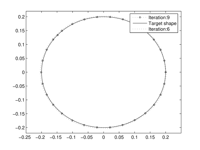
Figure 6.3: Case 1, $\alpha=1$, CPU time after 9 iterations: 37.235 second

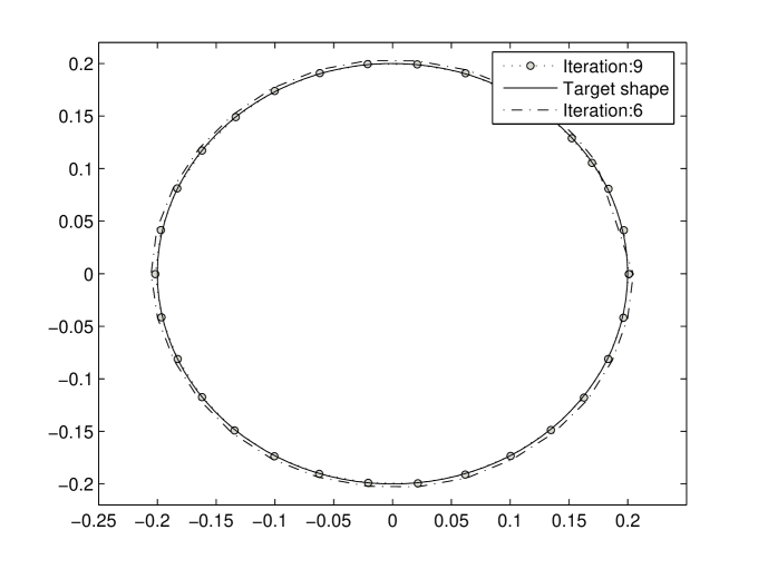
Figure 6.4: Case 1, $\alpha=0.1$, CPU time after 9 iterations: 36.125 second

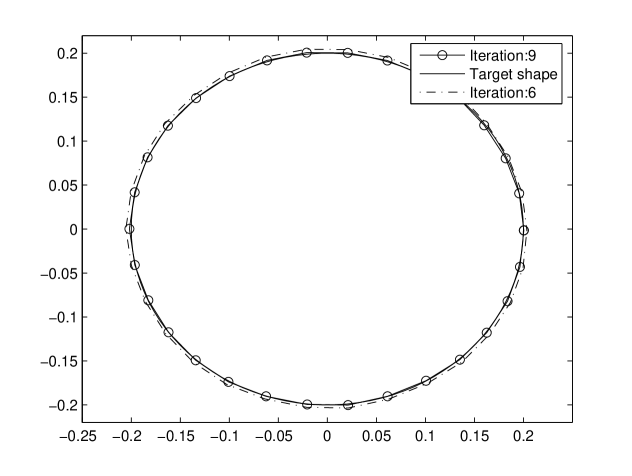
Figure 6.5: Case 1, $\alpha=0.01$, CPU time after 9 iterations: 37.14 second

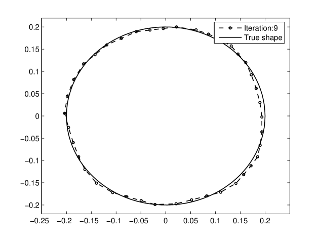
Figure 6.6: Case 1, $\alpha=0.001$, CPU time after 9 iterations: 47.375 second

In Case 1, Figure 6.3—Figure 6.6 give the comparison between the target shape with iterated shape for the viscosity coefficient $\alpha=1,0.1,0.01,0.001$, respectively. We can find that for $\alpha=1,0.1,0.01,$ we have nice reconstruction, but for $\alpha=0.001,$ the result is not so satisfied in Figure 6.6.

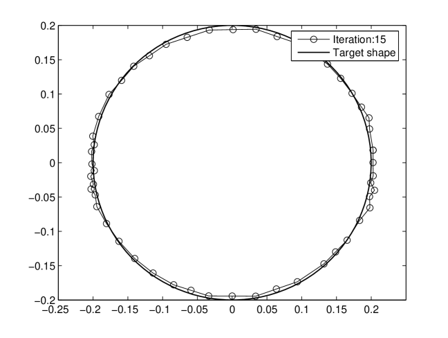
Figure 6.7: Case 2, $\alpha=1$, CPU time after 15 iterations: 64.11 second

Figure 6.8: Case 2, $\alpha=0.1$, CPU time after 15 iterations: 64.172 second

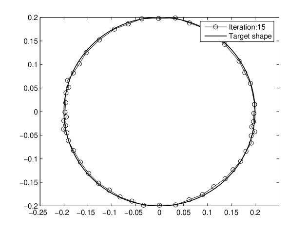
Figure 6.9: Case 2, $\alpha=0.01$, CPU time after 15 iterations: 66.141 second

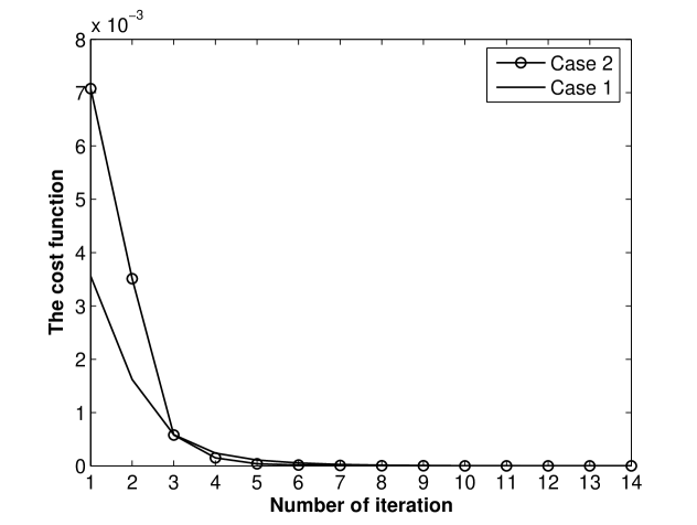
Figure 6.10: Convergence history of the cost function in two cases with $\alpha=0.01$.

In Case 2, Figure 6.7—Figure 6.9 represent the comparison between the target shape with iterated shape for the viscosity coefficient $\alpha=1,0.1,0.01$, respectively. It can be shown that for fixed viscosity, Case 1 has better reconstruction than Case 2, that’s to say, the iteration process depends on the choice of the initial shape.

Figure 6.10 shows the fast convergence of our cost function (6.4) in Case 1 and Case 2 for the viscosity $\alpha=0.01$.

Finally, the numerical examples show the feasibility of the proposed iteration algorithm and further research is necessary on efficient implementations.