Vortex state in a Fulde-Ferrell-Larkin-Ovchinnikov superconductor based on the quasiclassical theory

Abstract

We investigate the vortex state with Fulde-Ferrell-Larkin-Ovchinnikov (FFLO) modulations suggested for a high field phase of ${\rm CeCoIn_{5}}$. On the basis of the quasiclassical Eilenberger theory, we calculate the three dimensional structure of pair potentials, internal magnetic fields, paramagnetic moments, and electronic states, for the $s$-wave and the $d$-wave pairings comparatively. The $\pi$-phase shift of the pair potential at the FFLO nodal plane or at the vortex core induces sharp peak states in the local density of states, and enhances the local paramagnetic moment. We also discuss the NMR spectrum and the neutron scattering as methods to detect the FFLO structure.

I Introduction

The Fulde-Ferrell-Larkin-Ovchinnikov (FFLO) state ff ; lo is an exotic superconducting state expected to appear at low temperatures and high fields, when the paramagnetic depairing is significant due to the Zeeman effect under a magnetic field. In the FFLO state, since the Fermi surfaces for up-spin and down-spin electron bands are split by the Zeeman effect, Cooper pairs of up- and down-spins acquire non-zero momentum for the center of mass coordinate of the Cooper pair, inducing the spatial modulation of the pair potential. machida ; tachiki ; shimahara ; klein ; buzdin ; adachi ; ikeda The possible FFLO state is widely discussed in various research fields, ranging from superconductors in condensed matter, neutral Fermion superfluids in an atomic cloud, mizushima ; zwierlein ; partridge ; machida2006 to color superconductivity in high energy physics.casalbuoni

Experimentally, the FFLO state is suggested in a high field phase of a quasi-two dimensional (Q2D) heavy Fermion superconductor ${\rm CeCoIn_{5}}$. bianchi ; radovan Anomalous behaviors of the sound wave velocity, watanabe thermal conductivity, capan penetration depth,martin and the NMR spectrum kakuyanagi ; kumagai in the high field phase are considered as evidence of the FFLO structure. There, it is supposed that nodal planes of the pair potential run perpendicular to the vortex lines.

In theoretical studies, many calculations for the FFLO state have been done by neglecting vortex structure. However, we have to include the vortex structure in addition to the FFLO modulation, because the FFLO state appears at high fields in the mixed states.buzdin ; adachi ; ikeda Among the FFLO states, there are two possible spatial modulation of the pair potential $\Delta$. One is the Fulde-Ferrell (FF) state ff with phase modulation such as $\Delta\propto{\rm e}^{{\rm i}Qz}$, where $Q$ is the modulation vector of the FFLO states. The other is the Larkin-Ovchinnikov (LO) state lo with the amplitude modulation such as $\Delta\propto\sin Qz$, where the the pair potential shows the periodic sign change, and $\Delta=0$ at nodal planes. We discuss the case of the LO states in this paper, since some experimental watanabe ; capan ; kakuyanagi and theoretical buzdin ; ikeda works support the LO state (at least in low temperature region) for the FFLO states in ${\rm CeCoIn_{5}}$. In the FFLO vortex state, it is instructive to analyze the role of the nodal plane in the LO states, which may give a clue to obtain clear evidence of the FFLO states among the experimental data.

When we consider vortex structure in the LO state, there are two possible choices of the configuration for the vortex lines and the FFLO modulation. That is, the modulation vector of the FFLO state is parallel tachiki or perpendicular shimahara ; klein to the applied magnetic field. In our study, the former case is investigated by the quasiclassical theory. tachiki ; klein ; klein87 ; ichiokaS ; ichiokaD ; ichiokaMgB2 In a previous quasiclassical study by Tachiki et al. tachiki for this case, they calculate the structure of the FFLO modulation after reducing the FFLO states with Abrikosov vortex lattice to a problem of the one dimensional (1D) system along the magnetic field direction. There, the radial dependence from the vortex core could not be analyzed, since the spatial dependence of vortex is approximately changed to the averaged one. In our study, fully three dimensional (3D) structures of the vortex and the FFLO modulation are determined by the selfconsistent calculation based on the quasiclassical theory. That is, we also selfconsistently obtain the radial dependence around vortex in the FFLO vortex states, which was not done before.

On the other hand, the vortex and FFLO nodal plane structures in the FFLO state were calculated by the Bogoliubov de-Gennes (BdG) theory for a single vortex in a superconductor under a cylindrical symmetry situation. mizushima2 This study clarifies that the topological structure of the pair potential plays important roles to determine the electronic structures in the FFLO vortex state. The pair potential has $2\pi$-phase winding around the vortex line, and $\pi$-phase shift at the nodal plane of the FFLO modulation. These topologies of the pair potential structure affect the distribution of paramagnetic moment and low energy electronic states inside the superconducting gap. For an example, the paramagnetic moment is enhanced at the vortex core and the FFLO nodal plane. These structures are related to the bound states due to the $\pi$-phase shift of the pair potential.

The other method to microscopically study the vortex state is the calculations by the quasiclassical Eilenberger theory. In the calculation by the BdG theory, we have to assume a cylindrical symmetry and open boundary condition for the system, because of the limit of matrix size to numerically solve the BdG equation in the present status of the computers. However, using the Eilenberger theory in the limit $k_{\rm F}\xi\ll 1$ ($k_{\rm F}$ is Fermi wave number and $\xi$ is the superconducting coherence length), we are free from these restrictions. Therefore, we can discuss the cases of anisotropic pairing symmetry, such as $d$-wave pairing, and arbitrary shape Fermi surfaces, where we obtain broken cylindrical structures around vortices. Since we can consider the system of vortex lattice and periodic FFLO modulation by the periodic boundary condition, we can discuss the overlaps between tails of the neighbor vortex cores or FFLO nodal planes. These calculations for the periodic systems make us possible to estimate the resonance line shapes in the NMR experiments and form factors in the neutron scattering experiment.

The purpose of this paper is to investigate the 3D structures of the vortex and the FFLO nodal plane in the FFLO vortex state by the quasiclassical theory. We calculate the spatial structures of pair potentials, paramagnetic moments, internal magnetic fields and electronic states in the vortex lattice state under the given period of the FFLO modulation. From the results, we confirm the fundamental properties of the FFLO vortex states obtained by the BdG theory, and clarify the further details of the FFLO vortex states in the system of the vortex lattice and periodic FFLO modulation. Since the superconducting pairing symmetry of ${\rm CeCoIn_{5}}$ is suggested to be a $d$-wave with line nodes, we calculate both cases of the isotropic $s$-wave pairing and the anisotropic $d$-wave paring comparatively, in order to study the contribution of the pairing symmetry to the FFLO vortex state.ikeda ; Vorontsov In the calculation, we use the Q2D Fermi surface and a magnetic field is applied to the $ab$ plane, as is done for ${\rm CeCoIn_{5}}$. As possible experimental methods to detect the FFLO modulation, we discuss the NMR resonance line shape kakuyanagi and the neutron scattering experiments. We show that the spatial structure of the paramagnetic moment reflects the NMR resonance line shape in the NMR experiment observing Knight shift under an applied magnetic field.

After introducing the formulation for the calculation of the FFLO vortex structure by the quasiclassical theory including the paramagnetic effect in Sec. II, we investigate the spatial structure of the FFLO vortex states in Sec. III, and electronic states in Sec. IV. Using the calculated structure of the FFLO vortex states, we discuss the NMR resonance line shape in Sec. V and the neutron scattering in Sec. VI. The last section is devoted to the summary and discussions.

II Quasiclassical theory including paramagnetic effect

In this study for the FFLO vortex state, we take account of the paramagnetic depairing effect due to the Zeeman splitting term $\mu_{\rm B}B({\bf r})$ in addition to the orbital depairing effect by the vector potential ${\bf A}({\bf r})$. Therefore, Hamiltonian for the spin-singlet pairing superconductor is given by

$${\cal H}-\mu_{0}{\cal N}=\sum_{\sigma=\uparrow,\downarrow}\int{\rm d}^{3}{\bf r}\ \psi_{\sigma}^{\dagger}({\bf r})K_{\sigma}({\bf r})\psi_{\sigma}({\bf r})$$

$$\quad-\int{\rm d}^{3}{\bf r}_{1}\int{\rm d}^{3}{\bf r}_{2}\left\{\Delta({\bf r}_{1},{\bf r}_{2})\psi_{\uparrow}^{\dagger}({\bf r}_{1})\psi_{\downarrow}^{\dagger}({\bf r}_{2})\right.$$

$$\qquad\qquad\qquad\left.+\Delta^{\ast}({\bf r}_{1},{\bf r}_{2})\psi_{\downarrow}({\bf r}_{2})\psi_{\uparrow}({\bf r}_{1})\right\}$$ (1)

with

$$K_{\sigma}({\bf r})=\frac{\hbar^{2}}{2m}\left(\frac{\nabla}{\rm i}+\frac{2\pi}{\phi_{0}}{\bf A}\right)^{2}+\sigma\mu_{\rm B}B({\bf r})-\mu_{0},$$ (2)

the flux quantum $\phi_{0}$, and $\sigma=\pm 1$ for up/down spin electrons. In the following, length, temperature, Fermi velocity, magnetic field and vector potential are, respectively, scaled by $R_{0}$, $T_{c}$, $\bar{v}_{\rm F}$, $B_{0}$ and $B_{0}R_{0}$. Here, $R_{0}=\hbar\bar{v}_{\rm F}/2\pi k_{\rm B}T_{\rm c}$, $B_{0}=\hbar c/2|e|R_{0}^{2}$, and $\bar{v}_{\rm F}=\langle v_{\rm F}^{2}\rangle_{\bf k}^{1/2}$ is an averaged Fermi velocity on the Fermi surface. $\langle\cdots\rangle_{\bf k}$ indicates the Fermi surface average. Energy $E$, pair potential $\Delta$ and Matsubara frequency $\omega_{l}$ are scaled by $\pi k_{\rm B}T_{\rm c}$.

Using the quasiclassical Green’s functions $g(\omega_{l}+{\rm i}\tilde{\mu}B,{\bf k},{\bf r})$, $f(\omega_{l}+{\rm i}\tilde{\mu}B,{\bf k},{\bf r})$, $f^{\dagger}(\omega_{l}+{\rm i}\tilde{\mu}B,{\bf k},{\bf r})$, Eilenberger equations are given by tachiki ; klein ; klein87 ; ichiokaS ; ichiokaD ; ichiokaMgB2

$$\left\{\omega_{l}+{\rm i}\tilde{\mu}B+{\bf v}\cdot\left(\nabla+{\rm i}{\bf A}\right)\right\}f=\Delta({\bf r},{\bf k})g,$$

$$\left\{\omega_{l}+{\rm i}\tilde{\mu}B-{\bf v}\cdot\left(\nabla-{\rm i}{\bf A}\right)\right\}f^{\dagger}=\Delta^{\ast}({\bf r},{\bf k})g,$$

$${\bf v}\cdot{\nabla}g=\Delta^{\ast}({\bf r},{\bf k})f-\Delta({\bf r},{\bf k})f^{\dagger},$$ (3)

where $g=(1-ff^{\dagger})^{1/2}$, ${\rm Re}g>0$, $\Delta({\bf r},{\bf k})=\Delta({\bf r})\phi({\bf k})$, and $\tilde{\mu}=\mu_{\rm B}B_{0}/\pi k_{\rm B}T_{\rm c}$. In Eq. (3), ${\bf r}=({\bf r}_{1}+{\bf r}_{2})/2$ is the center of mass coordinate of the Cooper pair, and ${\bf k}=(k_{a},k_{b},k_{c})$ is a relative momentum of the Cooper pair. We set the pairing function $\phi({\bf k})=1$ in the $s$-wave pairing, and $\phi({\bf k})=\phi_{x^{2}-y^{2}}({\bf k})=\sqrt{2}(k_{a}^{2}-k_{b}^{2})/(k_{a}^{2}+k_{b}^{2})$ or $\phi({\bf k})=\phi_{xy}({\bf k})=2\sqrt{2}k_{a}k_{b}/(k_{a}^{2}+k_{b}^{2})$ in the $d$-wave pairing. The vector potential is given by ${\bf A}=\frac{1}{2}\bar{\bf B}\times{\bf r}+{\bf a}$ in the symmetric gauge, with an average flux density $\bar{\bf B}$. The internal field is obtained as ${\bf B}({\bf r})=\bar{\bf B}+\nabla\times{\bf a}$.

The pair potential is selfconsistently calculated by

$$\Delta({\bf r})=g_{0}N_{0}T\sum_{0\leq\omega_{l}\leq\omega_{\rm cut}}\left\langle\phi^{\ast}({\bf k})\left(f+{f^{\dagger}}^{\ast}\right)\right\rangle_{\bf k}$$ (4)

with $(g_{0}N_{0})^{-1}=\ln T+2T\sum_{0\leq\omega_{l}\leq\omega_{\rm cut}}\omega_{l}^{-1}$. We use $\omega_{\rm cut}=20k_{\rm B}T_{\rm c}$. The vector potential is selfconsistently determined by the paramagnetic moment and the supercurrent as

$$\nabla\times\nabla\times{\bf a}({\bf r})={\bf j}_{\rm s}({\bf r})+\nabla\times{\bf M}_{\rm para}({\bf r})\equiv{\bf j}({\bf r}),$$ (5)

where

$${\bf j}_{\rm s}({\bf r})=-\frac{2T}{{\tilde{\kappa}}^{2}}\sum_{0\leq\omega_{l}}\left\langle{\bf v}_{\rm F}{\rm Im}\{g\}\right\rangle_{\bf k}$$ (6)

is the supercurrent, and

$$M_{\rm para}({\bf r})=M_{0}\left(\frac{B({\bf r})}{\bar{B}}-\frac{2T}{\tilde{\mu}\bar{B}}\sum_{0\leq\omega_{l}}\left\langle{\rm Im}\left\{g\right\}\right\rangle_{\bf k}\right)$$ (7)

is the paramagnetic moment in the vortex lattice state. Here, the normal state paramagnetic moment $M_{0}=({\tilde{\mu}}/{\tilde{\kappa}})^{2}\bar{B}$, $\tilde{\kappa}=B_{0}/\pi k_{\rm B}T_{\rm c}\sqrt{8\pi N_{0}}$, $N_{0}$ is the density of states at the Fermi energy in the normal state.

When we calculate the electronic states, we solve Eq. (3) with $i\omega_{l}\rightarrow E+i\eta$. The local density of states (LDOS) is given by

$$N_{\sigma}({\bf r},E)=\langle{\rm Re}\{g(\omega_{l}+{\rm i}\sigma\tilde{\mu}B,{\bf k},{\bf r})|_{i\omega_{l}\rightarrow E+i\eta}\}\rangle_{\bf k}$$ (8)

for each spin component. We typically use $\eta=0.01$.

As a model of Fermi surface in ${\rm CeCoIn_{5}}$, we use a Q2D Fermi surface with rippled cylinder-shape, and the Fermi velocity is given by ${\bf v}_{\rm F}=(v_{a},v_{b},v_{c})\propto(\cos\theta,\sin\theta,\tilde{v}_{z}\sin k_{c})$ at the Fermi surface ${\bf k}_{\rm F}=(k_{a},k_{b},k_{c})\propto(k_{\rm F0}\cos\theta,k_{\rm F0}\sin\theta,k_{c})$ with $-\pi\leq\theta\leq\pi$ and $-\pi\leq k_{c}\leq\pi$. ichiokaMgB2 In our calculation we set $\tilde{v}_{z}=0.5$, so that the anisotropy ratio $\gamma=\xi_{c}/\xi_{ab}\sim\langle v_{c}^{2}\rangle_{\bf k}^{1/2}/\langle v_{a}^{2}\rangle_{\bf k}^{1/2}\sim 0.5$. A magnetic field is applied along the $a$ axis direction in our calculation. Thus, the coordinate $(x,y,z)$ for the vortex structure corresponds to $(b,c,a)$ of the crystal coordinate. In the $d$-wave pairing, the case of the pairing function $\phi_{x^{2}-y^{2}}$ ($\phi_{xy}$) corresponds to the configuration when $\bar{\bf B}$ is applied to the anti-nodal direction (the nodal direction) of the superconducting gap.

Figure 1: Configurations of the vortex lines and the FFLO nodal planes are schematically presented in the $xz$ plane including vortex lines (a) and in the $xy$ plane (b). The vortex distance is $a$ in the $x$ direction, and the distance between the FFLO nodal planes is $L/2$. The hatched region indicates the unit cell. In (a), along the trajectories presented by “$0\longrightarrow\pi$”, the pair potential changes the sign ($+\rightarrow-$) across the vortex line or across the FFLO nodal plane, due to the $\pi$-phase shift of the pair potential. Along the trajectory presented by “$0\longrightarrow 2\pi$”, the sign of the the pair potential does not change ($+\rightarrow+$) across the intersection point of the vortex line and the FFLO nodal plane, since the phase shift is $2\pi$. In (b), $\bullet$ indicates the vortex center. ${\bf u}_{1}-{\bf u}_{2}$ and ${\bf u}_{2}$ are unit vectors of the vortex lattice.

We solve Eq. (3) and Eqs. (4)-(7) alternately, and obtain selfconsistent solutions as in previous works, ichiokaS ; ichiokaD ; ichiokaMgB2 by fixing a unit cell of the vortex lattice and a period $L$ of the FFLO modulation. The unit cell of the vortex lattice is given by ${\bf r}=w_{1}({\bf u}_{1}-{\bf u}_{2})+w_{2}{\bf u}_{2}+w_{3}{\bf u}_{3}$ with $-0.5\leq w_{i}\leq 0.5$ ($i$=1, 2, 3), ${\bf u}_{1}=(a,0,0)$, ${\bf u}_{2}=(a/2,a_{y},0)$ and ${\bf u}_{3}=(0,0,L)$. Reflecting anisotropy ratio $\gamma$, we set $a_{y}/a=\sqrt{3}\gamma/2$ with $\gamma=0.5$. For the FFLO modulation, we assume $\Delta(x,y,z)=\Delta(x,y,z+L)$ and $\Delta(x,y,z)=-\Delta(x,y,-z)$. Then, $\Delta({\bf r})=0$ at the FFLO nodal planes $z=0$, and $\pm 0.5L$. These configurations of the FFLO vortex structure are schematically shown in Fig. 1, which show the unit cell in the $xz$ plane including vortex lines, and in the $xy$ plane.

We divide $w_{i}$ to $N_{i}$-mesh points in our numerical calculation, and obtain the quasiclassical Green’s functions, $\Delta({\bf r})$, $M_{\rm para}({\bf r})$ and ${\bf j}({\bf r})$ at each mesh point in the 3D space. Typically we set $N_{1}=N_{2}=N_{3}=31$. In the selfconsistent calculation of ${\bf a}$, we solve Eq. (5) in the Fourier space ${\bf q}_{m_{1},m_{2},m_{3}}$, taking account of the current conservation $\nabla\cdot{\bf j}({\bf r})=0$, so that the average flux density per unit cell of the vortex lattice is kept constant. The wave number ${\bf q}$ is discretized as

$${\bf q}_{m_{1},m_{2},m_{3}}=m_{1}{\bf q}_{1}+m_{2}{\bf q}_{1}+m_{3}{\bf q}_{3}$$ (9)

with integers $m_{i}$ ($i=1,2,3$), where ${\bf q}_{1}=(2\pi/a,-\pi/a_{y},0)$, ${\bf q}_{2}=(2\pi/a,\pi/a_{y},0)$, and ${\bf q}_{3}=(0,0,2\pi/L)$. The lattice momentum is defined as ${\bf G}({\bf q}_{m_{1},m_{2},m_{3}})=(G_{x},G_{y},G_{z})$ with $G_{x}=[N_{1}\sin(2\pi m_{1}/N_{1})+N_{2}\sin(2\pi m_{2}/N_{2})]/a$, $G_{y}=[-N_{1}\sin(2\pi m_{1}/N_{1})+N_{2}\sin(2\pi m_{2}/N_{2})]/2a_{y}$, and $G_{z}=N_{3}\sin(2\pi m_{3}/N_{3})/L$. We obtain the Fourier component of ${\bf a}({\bf r})$ as ${\bf a}({\bf q})={\bf j}^{\prime}({\bf q})/|{\bf G}|^{2}$, where ${\bf j}^{\prime}({\bf q})={\bf j}({\bf q})-{\bf G}\left({\bf G}\cdot{\bf j}({\bf q})\right)/|{\bf G}|^{2}$ ensuring the current conservation $\nabla\cdot{\bf j}^{\prime}({\bf r})=0$, and ${\bf j}({\bf q})$ is the Fourier component of ${\bf j}({\bf r})$ in Eq. (5).klein87 The final selfconsistent solution satisfies $\nabla\cdot{\bf j}({\bf r})=0$. When we solve Eq. (3) by the explosion method, klein87 ; ichiokaS ; ichiokaD ; ichiokaMgB2 we estimate $\Delta({\bf r})$ and ${\bf A}({\bf r})$ at arbitrary positions by the interpolation from their values at the mesh points, and by the periodic boundary condition of the unit cell including the phase factor due to the magnetic field.

III FFLO vortex structure

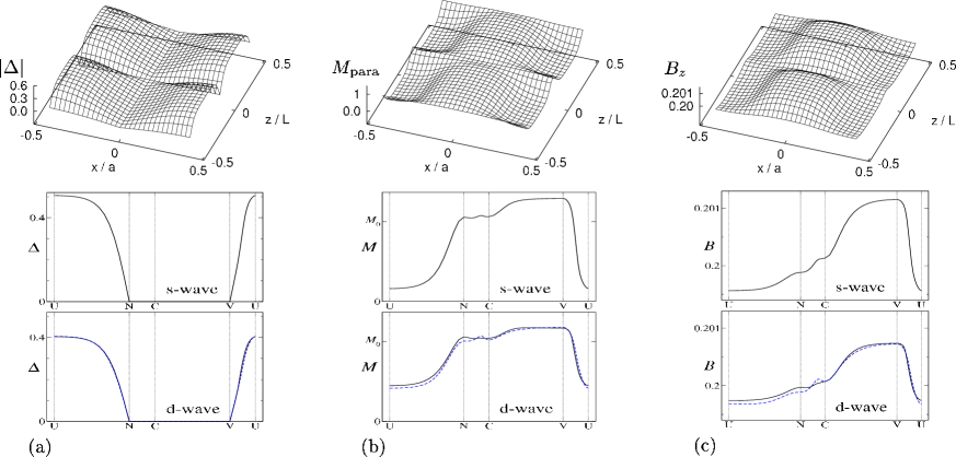
Figure 2: (color online) Spatial structure of the FFLO vortex state in the $xz$ plane at $\bar{B}=0.2B_{0}$, $T=0.1T_{\rm c}$ and $L=50R_{0}$. (a) Amplitude of the pair potential $|\Delta({\bf r})|$. (b) Paramagnetic moment $M_{\rm para}({\bf r})$. (c) Internal magnetic field $B_{z}({\bf r})$. The upper panels show the spatial variation within a unit cell [hatched region in Fig. 1(a)] for the $s$-wave pairing. The middle panels present the profiles along the path UNCVU shown in Fig. 1(a) for the $s$-wave pairing. The lower panels are the same as the middle panels, but for the $d$-wave pairing. The solid (dashed) lines are for the case when the applied field is applied to the anti-nodal (nodal) direction.

We consider the case of large GL parameter $\tilde{\kappa}=20$ and large paramagnetic contribution $\tilde{\mu}=1.7$. In these parameters, the upper critical field is suppressed to $H_{c2}(T=0.1T_{c})\sim 0.22B_{0}$, as a first order transition. We discuss the FFLO vortex state when we set $L=50R_{0}$ or $70R_{0}$ at $T=0.1T_{c}$ and $\bar{B}=0.2B_{0}$, giving $M_{0}=0.00139B_{0}$ and the vortex lattice constant $a=8.5R_{0}$.

In the upper panels of Fig. 2, we show the spatial structure of the FFLO vortex state within a unit cell in the slice of the $xz$ plane, i.e., the hatched region shown in Fig. 1(a). In the middle and lower panels of Fig. 2, the profiles of the spatial structure are presented along the path UNCVU shown in Fig. 1(a). The point C ($x=y=z=0$) is the intersection point of a vortex and a nodal plane. The point V ($x=y=0$ and $z=L/4$) is at the vortex center and far from the FFLO nodal plane. The point N ($x=a/2$, $y=z=0$) is at the FFLO nodal plane and outside of the vortex. The point U ($x=a/2$, $y=0$, $z=L/4$) is far from both the vortex and the FFLO nodal plane. In Fig. 2, in addition to the $s$-wave pairing case in the middle panels, we also present the $d$-wave pairing cases in the lower panels in order to show that the qualitative features of the FFLO vortex structure are independent of the pairing symmetry and the field orientation within the $ab$ plane.

Figure 2(a) shows the amplitude of the order parameter. In the upper panel, we see that $|\Delta({\bf r})|$ is suppressed near the vortex center at $x=y=0$ and the FFLO nodal plane at $z=0$, $\pm 0.5L$. Far from the FFLO nodal plane such as $z=0.25L$, $|\Delta({\bf r})|$ shows a typical profile of the conventional vortex. When we cross the vortex line or the FFLO nodal plane, the sign of $\Delta({\bf r})$ changes due to the $\pi$-phase shift of the pair potential as schematically shown in Fig. 1(a). In the profile of $|\Delta({\bf r})|$ presented in the middle and the lower panels of Fig. 2(a), $|\Delta({\bf r})|=0$ along the FFLO nodal plane NC and along the vortex line CV. While amplitude $|\Delta({\bf r})|$ in the $s$-wave pairing [middle panel] is larger than that in the $d$-wave pairing [lower panel], this is due to the difference of the ratio $\Delta(H=0)/T_{c}$ depending on the pairing symmetry.

Correspondingly, paramagnetic moment $M_{\rm para}({\bf r})/M_{0}$ is presented in Fig. 2(b). As is well-known as the Knight shift, the paramagnetic moment is suppressed in the spin-singlet pairing superconducting state. In the figures, we see that $M_{\rm para}({\bf r})$ is suppressed outside of the vortex and far from the FFLO nodal plane, as expected. However, $M_{\rm para}({\bf r})$ is enhanced at the vortex core or at the FFLO nodal plane, both in the $s$-wave and the $d$-wave pairings. The reason for these structures of $M_{\rm para}({\bf r})$ is discussed later in connection with the LDOS. At the FFLO nodal plane $M_{\rm para}({\bf r})\sim M_{0}$ [path NC in Fig. 2(b)]. Along the vortex line, $M_{\rm para}({\bf r})$ is enhanced more than $M_{0}$ far from the FFLO nodal planes [position V in Fig. 2(b)].

Figure 2(c) presents the $z$-component of the internal field, $B_{z}({\bf r})$. Due to the contribution of the enhanced $M_{\rm para}({\bf r})$, $B_{z}({\bf r})$ is enhanced at the FFLO nodal plane even outside of the vortex. A part of the contributions by $M_{\rm para}({\bf r})$ is compensated by the diamagnetic contribution, because the average flux density per unit cell of the vortex lattice in the $xy$ plane should conserve along the magnetic field direction. Therefore, due to the conservation, the enhancement of $B_{z}({\bf r})$ at the FFLO nodal plane [path NC in Fig. 2(c)] is smaller, compared with the enhancement of $M_{\rm para}({\bf r})$ at the FFLO nodal plane [path NC in Fig. 2(b)]. While $B_{z}({\bf r})$ is largely enhanced than $\bar{B}$ at the vortex core far from the FFLO nodal plane [position V in Fig. 2(c)], $B_{z}({\bf r})$ is not largely enhanced at the vortex core in the FFLO nodal plane [position C]. Therefore $B_{z}({\bf r})\sim\bar{B}=0.2$ at the FFLO nodal plane [path NC].

We compare the behaviors of the middle panels for the $s$-wave pairing and the lower panels for the $d$-wave pairing. The profile along the path VU is almost the same as that of the conventional vortex without FFLO modulation. Quantitatively, the variable ranges of $M_{\rm para}({\bf r})$ and $B_{z}({\bf r})$ are smaller in the $d$-wave pairing, compared with the $s$-wave pairing. In the lower panels, we also show the dependence on the relative angle of the magnetic field and the gap nodes. In any cases of pairings and the magnetic field directions, we see qualitatively the same behavior of the FFLO structure, i.e., $M_{\rm para}({\bf r})\sim M_{0}$ and $B_{z}({\bf r})\sim\bar{B}$. Therefore, if we study the dependence on the pairing symmetry and the magnetic field direction within the $ab$ plane, we need to carefully examine the quantitative difference of the FFLO structure in the calculation of the pair potential, the paramagnetic moment and the internal magnetic field. On the other hand, the dependences on the pairing symmetry appear more clearly in the structure of the electronic states in the vortex states.ichiokaD Therefore, we discuss the electronic structure in the FFLO vortex states in the next section.

IV Electronic structure in the FFLO vortex state

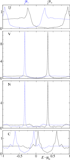
Figure 3: (color online) Spectrum of the LDOS for up-spin electrons $N_{\uparrow}(E,{\bf r})/N_{0}$ (solid lines) and for down-spin electrons $N_{\downarrow}(E,{\bf r})/N_{0}$ (dashed lines) in the $s$-wave pairing. $\bar{B}=0.2B_{0}$, $T=0.1T_{\rm c}$ and $L=50R_{0}$. From top panel to bottom, we present the LDOS at positions U, V, N, and C. Their locations are shown in Fig. 1(a).

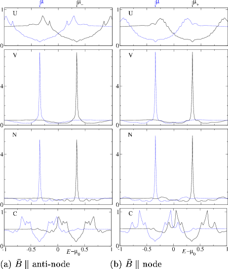
Figure 4: (color online) The same as Fig. 3, but in the $d$-wave pairing. (a) $\bar{{\bf B}}$ is applied to the anti-nodal direction. (b) $\bar{{\bf B}}$ is applied to the nodal direction.

The LDOS spectrum for up- and down-spin electrons are presented at some positions in Fig. 3 for the $s$-wave pairing and in Fig. 4 for the $d$-wave pairing. In the quasiclassical theory, $N_{\sigma}(E,{\bf r})$ are symmetric by $E\leftrightarrow-E$ in the absence of the paramagnetic effect ($\tilde{\mu}=0$). In the presence of the paramagnetic effect, the LDOS spectrum for up- (down-) spin electrons is shifted to positive (negative) energy by $\tilde{\mu}\bar{B}$ due to the Zeeman shift. In this case, we have a relation $N_{\uparrow}(E,{\bf r})=N_{\downarrow}(-E,{\bf r})$ within the quasiclassical theory.

Far from the FFLO nodal plane and outside of vortex, as shown in the spectrum of the top panel for the position U in Fig. 3, we see the superconducting full-gap structure of the $s$-wave pairing. There, small LDOS also appears at low energies inside the gap due to the low energy excitations extending from the vortex cores and the FFLO nodal planes at finite magnetic fields. Since the LDOS at $E<0$ ($E>0$) are occupied (empty) states, there is a relation between the LDOS spectrum and local paramagnetic moment as

$$M_{\rm para}({\bf r})=-\mu_{\rm B}\int_{-\infty}^{0}(N_{\uparrow}(E,{\bf r})-N_{\downarrow}(E,{\bf r})){\rm d}E.$$ (10)

In the full-gap case of the $s$-wave pairing, the difference of the occupation number between up- and down-spin electrons is small, since the LDOS below the gap are occupied similarly in $N_{\uparrow}(E,{\bf r})$ and $N_{\downarrow}(E,{\bf r})$. This is the reason why $M_{\rm para}({\bf r})$ is suppressed at the position U. Small but finite $M_{\rm para}({\bf r})$ comes from the small LDOS weight of low energy states inside the gap in the top panel of Fig. 3.

The LDOS spectra at the position V on the vortex center and at the position N on the FFLO nodal plane are, respectively, presented in the second and the third panels of Fig. 3. In these figures, $N_{\uparrow}(E,{\bf r})$ and $N_{\downarrow}(E,{\bf r})$, respectively, have a sharp peak at $E=\mu_{+}$ and $E=\mu_{-}$, with $\mu_{\pm}\equiv\mu_{0}\pm\tilde{\mu}\bar{B}$. These peaks are related to the topological structure of the pair potential, as schematically shown in Fig. 1. Since a vortex has phase winding $2\pi$, along the trajectory through the vortex center, $\Delta({\bf r})$ changes the sign by the $\pi$-phase shift across the vortex center. Also at the trajectory through the FFLO nodal plane, $\Delta({\bf r})$ changes the sign across the nodal plane. The bound states appear when the pair potential has the $\pi$-phase shift, and form the “zero-energy peak”. This peak is shifted to $E=\mu_{+}$ or $E=\mu_{-}$ due to the Zeeman effect.mizushima2 ; Takahashi Since the peak of the LDOS spectrum for up-spin electrons is an empty state ($E>0$) and the peak of the LDOS for down-spin electrons is an occupied state ($E<0$), $M_{\rm para}({\bf r})$ becomes large at these positions, from the relation in Eq. (10).

On the other hand, along the trajectory through the intersection point of a vortex and a nodal plane, $\Delta({\bf r})$ does not change the sign, because the phase shift is $2\pi$ by summing $\pi$ due to vortex and $\pi$ due to the nodal plane, as schematically shown in Fig. 1. Thus, the sharp peaks do not appear at $E=\mu_{\pm}$ as seen from the bottom panel of Fig. 3. Instead, $N_{\uparrow}(E,{\bf r})$ has two broad peaks at finite energies shifted upper or lower from $\mu_{+}$. In this situation, $M_{\rm para}({\bf r})$ is still large at position C, as in positions V and N, since the LDOS in both peaks are empty ($E>0)$ in $N_{\uparrow}(E,{\bf r})$, and occupied ($E<0$) in $N_{\downarrow}(E,{\bf r})$.

The differences of the $s$-wave and the $d$-wave pairings appear in the LDOS spectrum of the superconducting gap. At a zero field, the LDOS has the full-gap structure in the $s$-wave pairing, while it has a V-shape gap in the $d$-wave pairing with line nodes. Under the magnetic field, these features of the gap structure are smeared by low energy excitations under the magnetic field, but can be seen far from the vortex and the FFLO nodal plane, as is shown in top panels [position U] in Figs. 3 and 4. In the $d$-wave pairing, the LDOS spectrum has larger weight of low energy states within the gap [top panels in Fig. 4], and $M_{\rm para}({\bf r})$ is larger [position U in Fig. 2(b)], compared with the $s$-wave pairing. From Fig. 4, we see that in the $d$-wave pairing the LDOS structures at the vortex line and at the FFLO nodal plane are qualitatively the same as in the $s$-wave pairing. The sharp peak structure at $E=\mu_{\pm}$ appears in the LDOS at the vortex line [second panels] and at the FFLO nodal plane [third panels]. And the peak is split to two broad peaks, and shifted to upper or lower from $\mu_{\pm}$ at the intersection point of the vortex line and the FFLO nodal plane [bottom panels for the position C]. Figure 4 presents two cases of the magnetic field orientation, which show that the characteristic peak structures of the LDOS in the FFLO vortex structure do not significantly depend on the pairing symmetry and the relative angle of the magnetic field orientation and the gap-node direction.

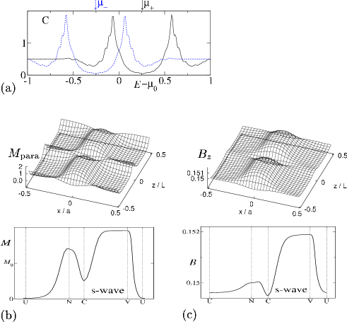
Figure 5: (color online) FFLO vortex structure at $\bar{B}=0.15B_{0}$, $T=0.1T_{\rm c}$ and $L=50R_{0}$ in the $s$-wave pairing. (a) Spectrum of the LDOS for up-spin electrons $N_{\uparrow}(E,{\bf r})/N_{0}$ (solid lines) and for down-spin electrons $N_{\downarrow}(E,{\bf r})/N_{0}$ (dashed lines) at the position C. (b) Paramagnetic moment $M_{\rm para}({\bf r})$. (c) Internal field $B_{z}({\bf r})$. The upper panels of (b) and (c) show the spatial variation within a unit cell. The lower panels present the profile along the path UNCVU.

In order to understand the relation between the LDOS and the paramagnetic moment, it is instructive to see the lower magnetic field case at $\bar{B}=0.15B_{0}$ shown in Fig. 5. Here, $a=9.8R_{0}$ and $M_{0}=0.00105B_{0}$. Figure 5(a) shows the LDOS at the position C. Compared with the LDOS in Fig. 3, the Zeeman shift $\tilde{\mu}\bar{B}$ of the spectrum is smaller. In this case, one of two broad peaks is occupied ($E<0$) and the other is empty ($E>0$) both for $N_{\uparrow}(E,{\bf r})$ and $N_{\downarrow}(E,{\bf r})$. Therefore, $M_{\rm para}({\bf r})$ is suppressed at the position C, i.e., the intersection point of the vortex line and the FFLO nodal plane, as shown in Fig. 5(b), while $M_{\rm para}({\bf r})$ is larger at the vortex line (position V) and at the FFLO nodal plane (position N). This structure corresponds to that obtained in the calculation by the BdG theory. mizushima2 Also in the spatial structure of the internal field, $B_{z}({\bf r})$ is suppressed at the position C as shown in Fig. 5(c) by the contribution from the spatial structure of $M_{\rm para}({\bf r})$.

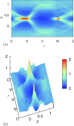
Figure 6: (color) Spectral evolution of the LDOS for up-spin electrons along the path CVUNC shown in Fig. 1(a). Density plot (a) and stereographic view (b) of $N_{\uparrow}(E,{\bf r})/N_{0}$ are presented in the $d$-wave pairing, when magnetic field $\bar{B}=0.2B_{0}$ is applied to the anti-nodal direction. $T=0.1T_{\rm c}$ and $L=50R_{0}$.

In Fig. 6, we show the spectral evolution of $N_{\uparrow}(E,{\bf r})/N_{0}$ around vortex and the FFLO nodal plane, when the pairing is $d$-wave and magnetic field is applied to the anti-nodal direction within $ab$ plain. We obtain similar spectral evolution also in the $s$-wave pairing. This spectral evolution is compared with that obtained by BdG theory in the $s$-wave pairing [see Fig. 3 in Ref. mizushima2, ]. The spectral structure is qualitatively good accordance with that. In the path VU, we see a typical spectral evolution of Caroli-de Gennes-Matricon states around the conventional vortex core. Takahashi ; Caroli ; CdGM ; Gygi ; Hayashi With aparting from the vortex center, vortex core states have higher angular momentum, and the energy levels are shifted to higher energy. Along the vortex line CV, moving from the nodal plane, two peak states at C are merged to the conventional vortex core states with $E=\mu_{+}$ at V. Also along the FFLO nodal plane NC, two peak states at the vortex center C are merged to the bound states with $E=\mu_{+}$ at the midpoint N of two vortices. The calculation for the midpoint was not done in the previous BdG calculation assuming cylindrical symmetry. mizushima2

V NMR spectrum

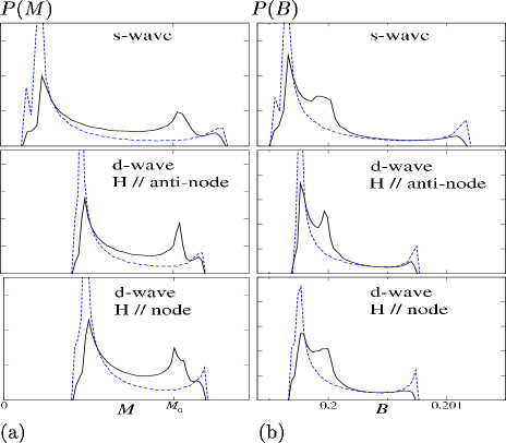
Figure 7: (color online) (a) Distribution function of the paramagnetic moment. We show $P(M)$ as a function of $M_{\rm para}$. (b) Distribution function of the internal magnetic field. We show $P(B)$ as a function of $B_{z}$. The solid (dashed) lines are for the vortex state with (without) the FFLO modulation. $\bar{B}=0.2B_{0}$, $T=0.1T_{c}$ and $L=50R_{0}$. The top panels are for the $s$-wave pairing. The middle (bottom) panels are for the $d$-wave pairing when the magnetic field is applied to the anti-nodal (nodal) directions. The heights of $P(M)$ and $P(B)$ are scaled so that $\int P(M){\rm d}M=\int P(B){\rm d}B=1$.

In the NMR experiment, resonance frequency spectrum of the nuclear spin resonance is determined by the internal magnetic field and the hyperfine coupling to the spin of the conduction electrons. Therefore, in a simple consideration, the effective field for the nuclear spin is given by $B_{\rm eff}({\bf r})=B({\bf r})+A_{\rm hf}M_{\rm para}({\bf r})$, where $A_{\rm hf}$ is a hyperfine coupling constant depending on species of the nuclear spins. The resonance line shape of NMR is given by

$$P(\omega)=\int\delta(\omega-B_{\rm eff}({\bf r})){\rm d}{\bf r},$$ (11)

i.e., the intensity at each resonance frequency $\omega$ comes from the volume satisfying $\omega=B_{\rm eff}({\bf r})$ in a unit cell. When the contribution of the hyperfine coupling is dominant, the NMR signal selectively detects $M_{\rm para}({\bf r})$. This is the experiment observing the Knight shift in superconductors. kohori ; tou As the NMR spectrum of the Knight shift, we calculate the distribution function $P(M)=\int\delta(M-M_{\rm para}({\bf r})){\rm d}{\bf r}$ from the spatial structure of the paramagnetic moment $M_{\rm para}({\bf r})$ shown in Fig. 2(b). We show $P(M)$ in Fig. 7(a). On the other hand, in the case of negligible hyperfine coupling, the NMR signal is determined by the internal magnetic field distribution. This resonance line shape is called “Redfield pattern” of the vortex lattice. In Fig. 7(b), we show the distribution function $P(B)=\int\delta(B-B_{z}({\bf r})){\rm d}{\bf r}$ calculated from the internal field $B_{z}({\bf r})$. In Fig. 7, the $s$-wave pairing case and two cases of the field orientations in the $d$-wave pairing are displayed.

First we discuss the line shape of the distribution function $P(M)$. The spectrum of $P(M)$ in the conventional vortex state without the FFLO modulation is shown by dashed lines in Fig. 7(a). There, the peak of $P(M)$ comes from the signal from the outside of the vortex core. The temperature dependence of this peak position $M$ gives Knight shift observed in the NMR experiments. kohori ; tou In our calculation, we confirm that $M$ is decreased from $M_{0}$ on lowering temperature below $T_{c}$. The spectrum of $P(M)$ has a tail toward larger $M$ by the vortex core contribution with large $M_{\rm para}({\bf r})$. The vortex core contribution is a 1D structure, their volume contribution is small in the spectrum, compared with the peak intensity due to the large volume contribution by the outside of the vortex. While $P(M)$ is slightly enhanced at the upper edge of $M$, this is the feature of the large paramagnetic effect. At the higher field near $H_{c2}$, the vortex core radius is expanded by the contribution of $M_{\rm para}({\bf r})$ enhanced at the vortex core, and the profile of $M_{\rm para}({\bf r})$ becomes flatter around the expanded vortex core region. These contributions slightly enhance $P(M)$ at the upper edge. This enhancement is not seen when the paramagnetic effect is not large, such as at lower fields.

In the vortex state with the FFLO modulation, the line shape $P(M)$ becomes double peak structure, as presented by solid lines in Fig. 7(a). The height of the main peak decreases, and there appears a new peak coming from the FFLO nodal plane near $M_{\rm para}\sim M_{0}$. This is because a part of contribution from the outside region of the vortex is shifted to the contribution of the FFLO nodal plane. The contribution from the two dimensional structure of the FFLO nodal plane appears in $P(M)$ more clearly than that of the 1D structure of the vortex line.

Second, we discuss the distribution function $P(B)$ of the internal magnetic field presented in Fig. 7(b). There, in the absence of the FFLO modulation (dashed lines), the Redfield pattern $P(B)$ has sharp peak corresponding the saddle point of the internal field distribution. The tail to higher $B$ comes from the increasing magnetic field around the vortex core. The small enhancement of $P(B)$ at the upper edge of $B$ is also due to the contribution from the flat profile of $M_{\rm para}({\bf r})$ around the expanded vortex core, mentioned above. In the presence of the FFLO modulation (solid lines), the height of the original peak is decreased, and a new peak appears at $B\sim\bar{B}=0.2B_{0}$ as the contribution of the FFLO nodal plane. As a feature of $P(B)$, the new peak appears near the main peak, compared with the line shape of $P(M)$.

In the $d$-wave pairing seen in lower two panels in Fig. 7, while the ranges for the variation of $M$ and $B$ are narrower, the double peak structures of the FFLO vortex state are seen as in the $s$-wave pairing. We also see that the shapes of $P(M)$ and $P(B)$ are not significantly affected by the orientation of the applied magnetic field within the $ab$ plane in the line node case of the $d$-wave pairing.

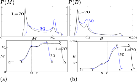
Figure 8: (color online) Structure of paramagnetic moment (a) and internal magnetic field (b) when $L/R_{0}=70$ (solid lines) and 30 (dashed lines) in the $d$-wave pairing when the magnetic field is applied to the anti-nodal direction. $\bar{B}=0.2B_{0}$ and $T/T_{c}=0.1$. The upper panels show the distribution function $P(M)$ or $P(B)$. The lower panels show the profile of $M_{\rm para}({\bf r})$ or $B_{z}({\bf r})$ along the path UNCVU.

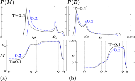
Figure 9: (color online) Structure of paramagnetic moment (a) and internal magnetic field (b) at $T/T_{c}=$0.1 (solid lines) and 0.2 (dashed lines) in the $d$-wave pairing when the magnetic field is applied to the anti-nodal direction. $\bar{B}=0.2B_{0}$ and $L=70R_{0}$. The upper panels show the distribution function $P(M)$ or $P(B)$. The lower panels show the profile of $M_{\rm para}({\bf r})$ or $B_{z}({\bf r})$ along the path UNCVU.

Next, we discuss how the spectra of $P(M)$ and $P(B)$ depend on the period $L$ of the FFLO modulation, and on the temperature $T$. The $L$-dependences of $P(M)$ and $P(B)$ are shown in the upper panels of Fig. 8, with the profiles of $M_{\rm para}({\bf r})$ and $B_{z}({\bf r})$ in the lower panels. With decreasing $L$, the new peak of the FFLO nodal plane is enhanced both in $P(M)$ and $P(B)$, since the relative weight of volume contribution by the FFLO nodal plane increases in the distribution functions. As is seen from the profile along the path UN in the lower panel of Fig. 8, the effective width of FFLO nodal plane where $M_{\rm para}({\bf r})$ is enhanced near the FFLO nodal plane [position N] does not significantly change. Instead, the width of the region [around position U] with low $M_{\rm para}({\bf r})$ and $B_{z}({\bf r})$, outside of the effective FFLO nodal plane width, becomes shorter, when $L$ decreases.

The temperature dependences of $P(M)$ and $P(B)$ are shown in the upper panels of Fig. 9, with the profiles of $M_{\rm para}({\bf r})$ and $B_{z}({\bf r})$ in the lower panels. In the spectra of $P(M)$ and $P(B)$, the height of the new peak due to the FFLO nodal plane becomes higher with increasing $T$. This is because the effective width of FFLO nodal plane becomes larger at higher $T$, since slope of $M_{\rm para}({\bf r})$ and $B_{z}({\bf r})$ from the FFLO nodal plane decreases as shown in the lower panel of Fig. 9 [see slope around the position N in the path UN]. This enhancement of the new peak of the FFLO nodal plane at higher $T$ comes from the increase of the effective coherence length. On the other hand, the slight enhancement of $P(M)$ and $P(B)$ at the upper edge, which appears even in the absence of the FFLO modulation, is smeared at higher $T$. This difference of the $T$-dependence can be used to distinguish the origin of the new peak observed in experiments. If the new peak becomes eminent at higher $T$, the origin of the new peak is the FFLO nodal plane. If the new peak becomes smeared at higher $T$, it may be an enhancement of the upper edge due to the paramagnetic vortex core effect. We also see that the main peak shifts to higher $M$ in $P(M)$ with increasing $T$, since $M_{\rm para}({\bf r})$ outside of vortex [around position U] is shifted to higher.

The experimental observation of the NMR resonance line shape was used to identify the FFLO phase in ${\rm CeCoIn_{5}}$. kakuyanagi There, the NMR spectrum shows the double peak structure in the FFLO phase, appearing new peak in addition to the main peak in the vortex state. This new peak is considered as a contribution of the FFLO nodal plane. This double peak structure is qualitatively reproduced by our calculation. In this status, our results may be qualitatively compared to the experimental data, since we did not perform fine tunings of parameters such as $L$, for the reason that we need further heavy calculations. The mechanism of rf-field penetration in the FFLO state kakuyanagi may further modify the NMR spectrum from the original $P(M)$. In the experimental data, the height of the new peak increases at higher $T$ in the NMR spectrum. kakuyanagi This feature is qualitatively consistent with the $T$-dependence in our results shown in Fig. 9, while it is an open question how $L$ increases as a function of $T$. It indicates that, among the $T$- and $L$-dependences discussed in Figs. 8 and 9, the contribution of the $T$-dependence seems to be dominant than the $L$-dependence in the increasing $T$ process.

VI Neutron scattering

Figure 10: Factor $|F_{h,k,l}|^{2}$ for the intensity of the neutron scattering, calculated from the internal magnetic field $B_{z}({\bf r})$ (a) or from the paramagnetic moment $M_{\rm para}({\bf r})$ (b) in the $d$-wave pairing when the magnetic field is applied to the anti-nodal direction. $|F_{h,k,l}|^{2}$ is plotted as a function of $l$ for $(h,k)=(1,0)$, $(1,1)$ and $(2,0)$. In (b), we also show $|F_{h,k,l}|^{2}$ for $(h,k)=(0,0)$. $\bar{B}=0.2B_{0}$, $T=0.1T_{c}$ and $L=70R_{0}$. Since the period of the FFLO modulation is $L/2$ for $B_{z}({\bf r})$ and $M_{\rm para}({\bf r})$ along the $z$ direction, the diffraction peaks appear at spots with even $l$.

The modulation of the internal magnetic field $B_{z}({\bf r})$ may be observed by the neutron scattering. If the periodic modulation along the $z$-direction is observed, it can be direct evidence of the FFLO modulation. Therefore, we discuss the neutron scattering in the FFLO vortex state. The intensity of the $(h,k,l)$-diffraction peak is given by $I_{h,k,l}=|F_{h,k,l}|^{2}/|q_{h,k,l}|$ with the wave vector ${\bf q}_{h,k,l}$ given in Eq. (9). Here we write $(m_{1},m_{2},m_{3})=(h,k,l)$ following notations of the neutron scattering. The Fourier component $F_{h,k,l}$ is given by $B_{z}({\bf r})=\sum_{h,k,l}F_{h,k,l}\exp({\rm i}{\bf q}_{h,k,l}\cdot{\bf r})$. In Fig. 10(a), we present $l$-dependence of $|F_{h,k,l}|^{2}$ for $(h,k)=(1,0)$, $(1,1)$ and $(2,0)$. The spot at $(h,k,l)=(1,0,0)$ and $(0,1,0)$ is used to determine the configuration and the orientation of the vortex lattice in the experiment of the small angle neutron scattering (SANS), and the higher component $F_{h,k,0}$ is used to estimate the structure of the internal magnetic field $B_{z}({\bf r})$. kealey It is noted that $F_{0,0,0}=\bar{B}$ and $F_{0,0,l}=0$ for $l\neq 0$, because average flux density $\bar{B}$ within the unit cell of the vortex lattice is constant along the $z$-direction. Therefore, to detect the FFLO modulation, we have to use the spot $(1,0,2)$, which has largest intensity among the spots related to the FFLO modulation. The spot $(1,0,2)$ is next to the spot $(1,0,0)$, which is used in the conventional SANS experiment to observe the stable vortex lattice configuration.

If the spins of the paramagnetic moment $M_{\rm para}({\bf r})$ strongly couple to the lattice modulation, it is possible to observe the structure of the paramagnetic moment through the lattice modulation by the neutron scattering. In this case, the Fourier component of the neutron scattering is given by $M_{\rm para}({\bf r})=\sum_{h,k,l}F_{h,k,l}\exp({\rm i}{\bf q}_{h,k,l}\cdot{\bf r})$. In Fig. 10(b), we present $|F_{h,k,l}|^{2}$ calculated from $M_{\rm para}({\bf r})$. Since $F_{0,0,l}$ ($l\neq 0$) is not zero in this case, the intensity at $(0,0,l)$ is larger than that at $(1,0,l)$ for the same $l$.

VII Summary and discussion

We investigated roles of the vortex and the FFLO nodal plane in the FFLO state, based on the quasiclassical Eilenberger theory. We selfconsistently calculated fully 3D spatial structure of the pair potential, the internal magnetic field, the paramagnetic moment, and local electronic states in the vortex lattice state under given period of the FFLO modulation $L$. We have seen that the topological structure of the pair potential determines the qualitative structure in the FFLO vortex state. At the FFLO nodal plane or at the vortex core, the $\pi$-phase shift of the pair potential gives rise to the sharp peaks in the local density of states, and enhances the local paramagnetic moment. Based on these results, we also discuss the experiments of NMR spectrum and neutron scattering, to identify characteristic behaviors in the FFLO states.

In this work, we calculate the FFLO vortex structure both in the isotropic $s$-wave paring and in the anisotropic $d$-wave pairing with line nodes, when the FFLO nodal planes are perpendicular to the vortex direction. If we compare the FFLO vortex states under the same FFLO modulation period, we see that even in the $d$-wave pairing the qualitative structures of the FFLO vortex state are the same as in the $s$-wave pairing, and do not significantly depend on the relative angle between the applied magnetic field direction and the node direction within the $ab$ plane. This is because qualitative features reported in this paper come from the topological structure of $\Delta({\bf r})$. Quantitatively, the dependences of the FFLO vortex state on the pairing symmetry or the magnetic field direction relative to the node of the superconducting gap are important features to characterize the FFLO vortex state.ikeda ; miranovic ; adachiM For the purpose, we need estimates of the optimized FFLO period $L$ and the phase diagram of the FFLO state in the mixed state. These calculations belong to future works within our framework of the selfconsistent calculations for the 3D structure of the FFLO vortex states. However, qualitative features do not significantly depend on this process. We did some calculations for different $L$, and confirmed that our results reported in this paper are qualitatively unchanged as for the FFLO vortex structure, because they come from the topological structure of the FFLO states, as discussed above.

Compared to results in the previous work by BdG theory, mizushima2 we obtain qualitatively the same features of the paramagnetic moment and local electronic states around vortices and FFLO nodal planes in the quasiclassical calculation. We note that these qualitative features by the $\pi$-phase shift of the pair potential were confirmed in this study also for the cases of $d$-wave pairing and the Q2D Fermi surface with parallel applied fields along $ab$ plane, which is not considered in the previous work by BdG theory assuming cylindrical symmetry structure and open boundary conditions. In this quasiclassical calculation with periodic boundary condition for the vortex lattice and FFLO modulation, we can take account of contributions by overlapping of electronic states from neighbor vortices or FFLO nodal planes. For example, we can discuss local structure at the mid-point between neighbor vortices. Compared with the previous quasiclassical work,tachiki since we calculate fully 3D structure of the FFLO vortex states without mapping to 1D problem, we can explicitly analyze the contribution of the vortex lines in the FFLO vortex states. Thus, we can quantitatively estimate the spatial structure around vortices along the radial direction, including the vortex structure within the FFLO nodal plane. There, we see exotic structure at the intersection point of vortex and FFLO nodal plane. By this 3D calculation of the FFLO vortex states, we can evaluate the NMR spectrum and form factors of neutron scattering, including vortex contributions in the FFLO states.

From the spatial structure of the paramagnetic moment in the FFLO vortex state, we can estimate the NMR spectrum in the Knight shift experiment. In the FFLO state, we obtain double peak structure of the NMR spectrum, as observed in the FFLO state of ${\rm CeCoIn_{5}}$, kakuyanagi and discuss the dependences on the temperature and on the FFLO period. From the spatial structure of the internal magnetic field, we also discuss the neutron scattering in the vortex states as methods to detect the FFLO structure. Since this is a direct observation of the FFLO modulation, we hope that this feature will be observed in experiments to confirm the FFLO states.

- (1) P. Fulde and R.A. Ferrell, Phys. Rev. 135, A550 (1964).
- (2) A.I. Larkin and Y.N. Ovchinnikov, Sov. Phys. JETP 20, 762 (1965).
- (3) K. Machida and H. Nakanishi, Phys. Rev. B 30, 122 (1984).
- (4) M. Tachiki, S. Takahashi, P. Gegenwart, M. Weiden, M. Lang, C. Geibel, F. Steglich, R. Modler, C. Paulsen, and Y. Onuki, Z. Physik B 100, 369 (1996).
- (5) H. Shimahara, Phys. Rev. B 50, 12760 (1994).
- (6) U. Klein, D. Rainer, and H. Shimahara, J. Low Temp. Phys. 118, 91 (2000).
- (7) M. Houzet and A. Buzdin, Phys. Rev. B 63, 184521 (2001).
- (8) H. Adachi and R. Ikeda, Phys. Rev. B 68, 184510 (2003).
- (9) R. Ikeda and H. Adachi, Phys. Rev. B 69, 212506 (2004).
- (10) T. Mizushima, K. Machida, and M. Ichioka, Phys. Rev. Lett. 94, 060404 (2005).
- (11) M.W. Zwierlein, A. Schirotzek, C.H. Schunck, and W. Ketterle, Science 311, 492 (2006).
- (12) G.B. Partridge, W. Li, R.I. Kamar, Y. Liao, R.G. Hulet, Science 311, 503 (2006).
- (13) K. Machida, T. Mizushima, and M. Ichioka, Phys. Rev. Lett. 97, 120407 (2006), and references cited therein.
- (14) R. Casalbuoni and G. Nardulli, Rev. Mod. Phys. 76, 263 (2004).
- (15) A. Bianchi, R. Movshovich, C. Capan, P.G. Pagliuso, and J.L. Sarrao, Phys. Rev. Lett. 91, 187004 (2003).
- (16) H. A. Radovan, N.A. Fortune, T.P. Murphy, S.T. Hannahs, E.C. Palm, S.W. Tozer, and D. Hall, Nature (London) 425, 51 (2003).
- (17) T. Watanabe, Y. Kasahara, K. Izawa, T. Sakakibara, Y. Matsuda, C. J. van der Beek, T. Hanaguri, H. Shishido, R. Settai, and Y. Onuki, Phys. Rev. B 70, 020506(R) (2004).
- (18) C. Capan, A. Bianchi, R. Movshovich, A.D. Christianson, A. Malinowski, M.F. Hundley, A. Lacerda, P.G. Pagliuso, and J.L. Sarrao, Phys. Rev. B 70, 134513 (2004).
- (19) C. Martin, C.C. Agosta, S.W. Tozer, H.A. Radovan, E.C. Palm, T.P. Murphy, and J.L. Sarrao, Phys. Rev. B 71, 020503(R) (2005).
- (20) K. Kakuyanagi, M. Saitoh, K. Kumagai, S. Takashima, M. Nohara, H. Takagi, and Y. Matsuda, Phys. Rev. Lett. 94, 047602 (2005).
- (21) K. Kumagai, M. Saitoh, T. Oyaizu, Y. Furukawa, S. Takashima, M. Nohara, H. Takagi, and Y. Matsuda, Phys. Rev. Lett. 97, 227002 (2006).
- (22) U. Klein, J. Low Temp. Phys. 69, 1 (1987).
- (23) M. Ichioka, N. Hayashi, and K. Machida, Phys. Rev. B 55, 6565 (1997).
- (24) M. Ichioka, A. Hasegawa, and K. Machida, Phys. Rev. B 59, 184 (1999); 59, 8902 (1999).
- (25) M. Ichioka, K. Machida, N. Nakai, and P. Miranović, Phys. Rev. B 70, 144508 (2004).
- (26) T. Mizushima, K. Machida, and M. Ichioka, Phys. Rev. Lett. 95, 117003 (2005).
- (27) A.B. Vorontsov, J.A. Sauls, and M.J. Graf, Phys. Rev. B 72, 184501 (2005).
- (28) M. Takahashi, T. Mizushima, M. Ichioka, and K. Machida, Phys. Rev. Lett. 97, 180407 (2006).
- (29) C. Caroli, J. Matricon: Phys. Kondens. Mater. 3, 380 (1965).
- (30) C. Caroli, P.-G. de Gennes, J. Matricon: Phys. Lett. 9, 307 (1964).
- (31) F. Gygi, M. Schlüter: Phys. Rev. Lett. 65, 1820 (1990); Phys. Rev. B 41, 822 (1990).
- (32) N. Hayashi, T. Isoshima, M. Ichioka, K. Machida: Phys. Rev. Lett. 80, 2921 (1998).
- (33) Y. Kohori, Y. Yamato, Y. Iwamoto, T. Kohara, E.D. Bauer, M.B. Maple, and J.L. Sarrao, Phys. Rev. B 64, 134526 (2001).
- (34) H. Tou, K. Ishida, and Y. Kitaoka, J. Phys. Soc. Jpn. 74, 1245 (2005).
- (35) P.G. Kealey, T.M. Riseman, E.M. Forgan, L.M. Galvin, A.P. Mackenzie, S.L. Lee, D.McK. Paul, R. Cubitt, D.F. Agterberg, R. Heeb, Z.Q. Mao, and Y. Maeno, Phys. Rev. Lett. 84, 6094 (2000).
- (36) P. Miranović, N. Nakai, M. Ichioka, and K. Machida, Phys. Rev. B 68, 052501 (2003).
- (37) H. Adachi, P. Miranović, M. Ichioka, and K. Machida, Phys. Rev. Lett. 94, 067007 (2005).