Testing turbulence model at metric scales with mid-infrared VISIR images at the VLT

Abstract

We probe turbulence structure from centimetric to metric scales by simultaneous imagery at mid-infrared and visible wavelengths at the VLT telescope and show that it departs significantly from the commonly used Kolmogorov model. The data can be fitted by the von Kármán model with an outer scale of the order of 30 m and we see clear signs of the phase structure function saturation across the 8-m VLT aperture. The image quality improves in the infrared faster than the standard $\lambda^{-1/5}$ scaling and may be diffraction-limited at 30-m apertures even without adaptive optics at wavelengths longer than 8 micron.

1 Introduction

As the ground-based telescopes become bigger, more emphasis is made on studying and modeling atmospheric optical distortions at large spatial scales. This knowledge is required, e.g. for specifying the stroke of deformable mirrors in adaptive optics or the range of fringe-trackers in interferometers. Moreover, the size of the atmospheric coherence length exceeds 1 m at infrared (IR) wavelengths. Thus, even classical long-exposure imagery in the IR is affected by the departures of turbulence statistics from the standard Kolmogorov model (variance proportional to the 5/3 power of the baseline) which was so successfully used in the visible range.

Optical path-length fluctuations were measured with long-baseline interferometers, but the published results are controversial. Saturation of the fringe motions at baselines from 8 m to 16 m was first observed by Mariotti & Di Benedetto (1984). Later, Davis et al. (1995) found a strong departure from the Kolmogorov law and a saturation of the path-length fluctuations at the 80-m baseline at a level of about 10 $\mu$m rms. On the other hand, Colavita et al. (1987) have not found any departure from the Kolmogorov law at baselines up to 12 m by doing a temporal analysis of the fringe motion, and Nightingale & Buscher (1991) reached the same conclusion from interferometric measurements of the fringe motion in a 4-m telescope aperture. The controversy could be caused by the use of the frozen-flow hypothesis in the interpretation of fringe motion on a single baseline. Another reason is the difficulty in separating fringe motion caused by the atmosphere from the mechanical noise due to instrument instabilities, tracking, etc.

Turbulence outer scale $L_{0}$ can be evaluated from the covariances of the image motion in small telescopes, as implemented in the GSM instrument (Ziad et al., 2000), or from the analysis of adaptive-optics data, e.g. by Fusco et al. (2004). These methods use the von Kármán (VK) turbulence spectrum (cf. Appendix A) and adjust its parameters $(r_{0},L_{0})$ to fit the data. Measurements with the GSM at different sites show that typical $L_{0}$ values are of the order of 20 m. Maire et al. (2006) compared directly fringe motion in a long-baseline interferometer with the $L_{0}$ measured by GSM and found a good agreement.

This short and non-exhaustive review demonstrates that further work on characterizing large-scale turbulence structure is needed. A direct comparison of mid-IR and optical images at a large telescope offers a new, independent way to probe turbulence models at spatial scales from centimeters to meters. To our knowledge, no such work has been done previously, so we made an experiment at the Very Large Telescope (VLT) located at the ESO observatory Cerro Paranal in Chile. The main purpose of this experiment is to evaluate the atmospheric phase structure function (SF) and to check if the VK model is adequate. So far, the mathematically convenient VK model has been used without being actually tested.

The experiment is described in Sect. 2. The results are presented in Sect. 3 and the conclusions are given in Sect. 4. Appendices contain some technical material. For reader’s convenience we reproduce the formulation of atmospheric models in Appendix A.

2 Experiment description

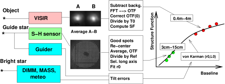
Figure 1: Overview of the experiment and data interpretation.

2.1 From PSF to structure function

It is well known that the modulus of the long-exposure optical transfer function (OTF) $T({\bf f})$ in a perfect telescope is related to the atmospheric SF $D_{\varphi}({\bf r})$ as (Tatarskii, 1961; Roddier, 1981)

$$T({\bf f})=T_{0}({\bf f})\exp[-0.5D_{\varphi}(\lambda{\bf f})],$$ (1)

where $T_{0}({\bf f})$ is the diffraction-limited OTF, ${\bf f}$ is the vector of spatial frequency on the sky in rad^-1, $f=|{\bf f}|$, $\lambda$ is the imaging wavelength and ${\bf r}$ is the baseline vector. This relation can be inverted to reconstruct $D_{\varphi}({\bf r})$ from the known image point spread function (PSF). However, it is only feasible at the baselines ${\bf r}=\lambda{\bf f}$ where $D_{\varphi}({\bf r})$ is not very large or small, otherwise $T({\bf f})$ is close to either 1 or 0 and the sensitivity to the atmospheric turbulence is lost. In the visible range, the method probes centimetric and decametric scales, in the mid-IR it is sensitive to the metric scales because $\lambda$ is much larger.

The 8-m VLT telescope offers a unique platform for our experiment with access to metric baselines. The aberrations are removed by active optics and the turbulence inside the dome is low, ensuring that the image blur is dominated by the atmospheric seeing. Optical images as small as $0.18^{\prime\prime}$ FWHM have been recorded under exceptional conditions, proving that the VLT intrinsic quality is nearly ideal even in the visible range. For our purpose, the mid-IR imager VISIR installed at the Cassegrain focus of the UT3 telescope is the best choice.

A deeper analysis of the mid-IR images shows that some departures from the ideal-telescope model (1) are inevitable. Residual image motion (tilt) is the largest source of uncertainty, as it can cause additional blur (e.g. wind shake), while, on the other hand, part of the atmospheric tilt is removed by guiding. Residual aberrations in the VLT optics and instrument can add something to the atmospheric PSF, too. Therefore, opto-mechanical wave-front distortions of instrumental nature cannot be separated cleanly from the large-scale atmospheric distortions. In this respect our new experiment is not fundamentally different from long-baseline interferometers, but it was worth trying nevertheless because instrumental effects in both cases are different.

2.2 Overview

Table 1: Instrument parameters

Instrument	VISIR	VISIR	SH
Filter	PAH1	Q2	None
Aperture diam., m	8.115	8.115	0.34 square
$\lambda$/$\Delta\lambda$, $\mu$m	8.6/0.42	18.7/0.88	0.6/$\sim$0.3
Pixel scale, arcsec	0.075	0.075	0.280
Detector format	256$\times$256	256$\times$256	592$\times$573
Exposure time, s	30$\times$2	90$\times$1	$\sim$45
Chopping period, s	4	2	None

The overall scheme of the experiment is presented in Fig. 1. Two different stars are observed through the VLT: the object with VISIR, the guide star with the Shack-Hartmann (SH) sensor of the VLT active optics (AO) system. The same guide star is used for the guiding, called field stabilization. The angular distance between the object and the guide star was from $3^{\prime}$ to $5^{\prime}$. Details of the optical and IR imagery and data reduction are given below and in Table 1.

Data on the seeing and turbulence profile at the Paranal observatory are collected by the dedicated site monitor equipped with the Differential Image Motion Monitor (DIMM) (Sarazin & Roddier, 1990) and Multi-Aperture Scintillation Sensor (MASS) (Kornilov et al., 2003). The monitor points to a bright star near zenith and measures the total seeing $\epsilon$ and the seeing in the free atmosphere $\epsilon_{FA}$ produced by turbulence above 500 m. Naturally, $\epsilon_{FA}<\epsilon$ unless most turbulence is above 500 m. The VLT dome is higher than the DIMM tower, hence the seeing at VLT can be better than that measured by DIMM, but still worse or equal to $\epsilon_{FA}$. The MASS also measures the adaptive-optics time constant $\tau_{0}$ and a crude turbulence profile. The effective wind speed in the free atmosphere $\overline{V}$ was evaluated from the relation $\overline{V}=0.31r_{0,FA}/\tau_{0}$. The speed of the ground wind $V_{gr}$ was taken from the Paranal ambient conditions database.

2.3 Conditions of the experiment

Table 2: Night log

Date	Time	Air	$\epsilon$,	$\epsilon_{FA}$,	$\overline{V}$	$V_{gr}$
Jun 2006	UT	mass	′′	′′	m/s	m/s
19/20	23:38–23:44	1.7	1.38	0.63	30	5.6
21/22	1:40–1:49	1.5	1.21	0.68	13	2.5
22/23	23:07–23:16	1.1	0.54	0.27	16	6.4

Figure 2: Temporal evolution of the seeing $\epsilon$ and the seeing in the free atmosphere $\epsilon_{FA}$ as measured by DIMM and MASS respectively during the data acquisition periods on 3 nights. The seeing derived from the SH spots and reduced to zenith is over-plotted as large squares.

The data for this study have been obtained by A.S. on June 19, 21, and 22, 2006. Table 2 lists relevant average parameters for each data set. On all nights the sky was clear, with stable air temperature and very low humidity. Individual (non-averaged) data from DIMM and MASS are plotted in Fig. 2 to characterize the variability of the turbulence. The conditions were rather stable on all 3 nights, with the DIMM seeing always dominated by the ground layer. However, the seeing derived from the SH spots indicates that the ground seeing contribution at VLT was less than at DIMM on June 19/20 and 21/22.

2.4 VISIR data

Mid-IR images of bright stars were obtained with VISIR in two filters called PAH1 (8.6 $\mu$m) and Q2 (18.7 $\mu$m), cf. Table 1. A standard chopping-nodding technique was used. At each telescope position (nod), the image was shifted on the detector back and forth by modulation (chop) of the VLT secondary mirror M2 with a period of 2-4 s. The chop throw was $10^{\prime\prime}$ in the North-South direction, with a little pause to stabilize the image after each chop. For the PAH1 filter, for example, a total of 30 images with 2 s exposure in each chop position are taken to produce the data cube with cumulative exposure of 60 s. Then the telescope is moved by $10^{\prime\prime}$ to the East and a second data cube is taken. Here we do not take advantage of the nodding and analyze only the average difference between images in two chopping positions A and B. This A$-$B difference suppresses the background and its slow drifts. It is averaged over all image pairs in the cube and contains positive (A) and negative (B) images of the same star, considered here separately as two independent realizations of the PSF.

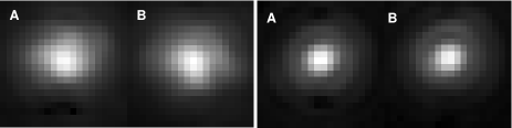
Figure 3: The pairs of positive and negative PSFs in the PAH1 filter registered with VISIR on June 21/22 (left, file 5) and June 22/23 (right, file 1). Only the central 20x20 pixels ($1.5^{\prime\prime}$) of each image are displayed with a square-root intensity stretch.

Figure 4: The cuts of the OTFs along $f_{x}$ axis for the VISIR images displayed in Fig. 3 (top – June 21/22, bottom – June 22/23). Asterisks – positive images, plusses – negative images. The line shows the diffraction-limited OTF $T_{0}(\lambda f)$.

The positive and negative PSFs are extracted as two 64x64 pixel ($4.8^{\prime\prime}$) subsections and processed in parallel. The background is computed in the corners of these images (outside the radius of 32 pixels) as a median and subtracted. For reference only, these PSFs are approximated with 2-dimensional Gaussians to determine the Full Width at Half Maximum (FWHM) $\epsilon_{l}$ and $\epsilon_{s}$ in the long and short axes. The ellipticity is computed as $e=(\epsilon_{l}-\epsilon_{s})/(\epsilon_{l}+\epsilon_{s})$ and the position angle $\theta$ of the long axis (counted from the $x$-axis counter-clockwise) is recorded as well.

Figure 5: The atmospheric OTF in the VISIR PAH1 filter obtained after correcting the observed OTFs for diffraction on June 22/23, file 1. All points are plotted without radial averaging (asterisks – image A, triangles – image B) to show the asymmetry. Compare with Fig. 4.

Figure 3 shows typical examples of the individual PSFs in the PAH1 filter on two nights. On June 21/22, the PSF is blurred by the turbulence. It is slightly elongated ($e=0.1...0.2$) and has some structure, different between positive and negative images. On June 22/23, under a better seeing, the PSF is closer to a diffraction-limited one, but still elongated ($e=0.08...0.12$). The elongation can be caused by a combination of several factors including some residual low-order aberrations, vibrations, etc. However, the dominant contribution to the image elongation is likely related to the tilt anisoplanatism between the guide star and the object, estimated in Appendix C. The direction of the elongation points approximately to the guide star.

Each PSF is Fourier-transformed and the normalized modulus of the FT is identified with the observed $T(f)$ (Fig.  4). The spatial frequencies $f$ are translated to the baselines $r=\lambda f$. A small correction is needed for the normalization (cf. Appendix B). The experimental OTF $T(f)$ is divided by the calculated $T_{0}(f)$ to obtain the atmospheric OTF and then the SF. In calculating $T_{0}(f)$, we use the pupil diameter $D=8.115$ m because it is not vignetted by the cold stop inside the VISIR instrument. Figure 5 shows the results of this division for the sharpest PAH1 image (compare with Fig. 4, bottom). The saturation of the OTF (hence SF) is obvious. The vertical spread is caused by the asymmetry and the differences between the images A and B.

Note that at small baselines the derived atmospheric OTFs and SFs are sensitive to the normalization errors, while at large baselines the experimental $T(f)$ becomes noisy and its modulus is biased by any image defects such as noise and bad pixels. For these reasons, we use for further analysis the baseline range from 0.4 m to 4 m, where $T(f)$ is most reliable. In the following, the asymmetry is neglected and the atmospheric SFs are calculated from the radially-averaged OTFs.

The data in the Q2 filter are rather noisy compared to the PAH1 filter. The PSFs are nearly diffraction-limited. At some nodding positions, the image is affected by bad detector pixels and/or horizontal stripes in the background. The OTFs registered on June 22/23 do not differ from the diffraction-limited ones within the errors. Therefore, no reliable estimates of the atmospheric SF are derived from the Q2 images on this night and we can only affirm that the phase fluctuations were much less than 1 rad at 18.7 $\mu$m.

2.5 Shack-Hartmann data

Long-exposure images from the Shack-Hartmann (SH) sensor were recorded quasi-simultaneously with the data. A typical exposure time is 45 s, but the SH “sees” the star only during 1/2 of the chopping cycle. On the other hand, the guiding was done continuously because the guiding “box” moved to compensate for the chopping.

Figure 6: The atmospheric OTF derived from the average SH spot de-convolved by the average reference spot (June 22/23, 23:07). The fitted Kolmogorov model is plotted in dashed line.

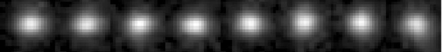
Figure 7: Mosaic of 8 individual good SH spots (June 22/23, 23:15), each in a $3^{\prime\prime}\times 3^{\prime\prime}$ field. The data are taken at air mass 1.1, with negligible atmospheric dispersion. The ellipticity of the average spot is $e=0.08$.

The SH images are “raw”, i.e. not corrected for bias, hot pixels, flat field, etc. The geometry of the lenslet array is square, with 24 spots across pupil diameter, hence sub-aperture size $d=0.34$ m. The pixel scale $0.30^{\prime\prime}$ was calculated from the opto-mechanical data of the SH sensor and telescope. However, the real pixel scale depends, among other things, on the actual distance between the lenslet array and the detector. So we obtained images of the known double star HIP 73246 with a separation of $3.512^{\prime\prime}$ measured by Hipparcos and derived the pixel scale $0.280^{\prime\prime}\pm 0.004^{\prime\prime}$ for the SH sensor at the Cassegrain focus of UT3.

The images of individual spots show various distortions and are all elongated in one direction due to the un-corrected atmospheric dispersion (except for the data taken near zenith). Initially, we selected for the analysis only the sharpest spots in each frame. The spots were extracted, over-sampled, re-centered and averaged. The influence of local CCD defects is reduced by the averaging. The modulus of the Fourier Transform $T({\bf f})$ of the average spot was calculated and normalized so that $T(0)=1$. Then it was divided by the diffraction-limited OTF for the square aperture $T_{0}({\bf f})=(1-|\lambda f_{x}/d|)\;(1-|\lambda f_{y}/d|)$, assuming $\lambda=0.6$ $\mu$m.

We presume that the elongation of the spots is caused primarily by the atmospheric dispersion. The long axis of $T({\bf f})$ is found by fitting a 2-dimensional Gaussian. The cut along this axis is fitted to the Kolmogorov atmospheric OTF (eq. 3), giving an estimate of the Fried’s parameter $r_{0,Kolm}$ and seeing $\epsilon_{SH}=0.98\lambda/r_{0,Kolm}$ (Fig. 6). The atmospheric SF at short baselines is derived from the same cut.

We found that even the sharpest spots were distorted by residual aberrations in the lenslets. A mosaic of selected sharp spots recorded under good seeing near zenith (Fig. 7) shows various degrees of distortion and elongation. This became apparent on June 22/23, under excellent conditions, when the SH measured a seeing of about $0.75^{\prime\prime}$, worse than the DIMM seeing. To overcome this problem, we used the image of the reference point source. A total of 306 sharpest reference spots were selected, re-centered and averaged in the same way as the star images. Then we re-processed the data by selecting the same spots and de-convolving them by the average reference spot instead of $T_{0}({\bf f})$. A good agreement between DIMM and SH was reached (Fig. 2).

3 Results

Table 3: Data log

Time	File	Filt	$\epsilon_{SH}$,	Image A			Image B			$r_{0}$,	$L_{0}$,
UT			′′	$\epsilon_{s}$	$e$	$\theta$	$\epsilon_{s}$	$e$	$\theta$	m	m
June 19/20
23:38	5	Q2	1.348	0.573	0.09	22	0.582	0.08	23	0.082	40
23:40	6	Q2	-	0.674	0.07	38	0.663	0.08	43	0.086	200
23:42	7	Q2	-	0.643	0.03	30	0.624	0.03	9	0.086	200
23:44	8	Q2	-	0.585	0.05	22	0.578	0.08	17	0.082	50
June 21/22
1:40	1	Q2	0.980	0.506	0.10	-25	0.513	0.09	-30	0.112	50
1:42	2	Q2	0.867	0.512	0.08	-19	0.530	0.08	-30	0.115	100
1:44	3	Q2	0.895	0.515	0.08	-19	0.529	0.06	-28	0.117	200
1:46	4	Q2	0.861	0.493	0.03	-20	0.505	0.02	-24	0.113	60
1:48	5	PAH1	0.719	0.379	0.10	-1	0.388	0.08	-9	0.110	30
1:49	6	PAH1	0.989	0.373	0.17	-7	0.400	0.19	3	0.111	40
June 22/23
23:07	1	PAH1	0.583	0.239	0.08	23	0.247	0.09	21	0.181	35
23:08	2	PAH1	0.575	0.245	0.12	32	0.251	0.09	22	0.182	40:
23:11	3	Q2	0.580	0.457	0.02	14	0.456	0.01	27	0.186	60:
23:12	4	Q2	0.614	0.455	0.02	20	0.454	0.02	8	0.186	60:
23:14	5	Q2	0.584	0.448	0.04	20	0.459	0.02	17	0.194	200:
23:16	6	Q2	0.584	0.451	0.02	4	0.448	0.02	14	0.194	200:

The results of image processing are gathered in the Table 3. The time (to 1 min) refers to the end of each acquisition. The seeing at 0.6 $\mu$m estimated from the SH spots $\epsilon_{SH}$ is listed as well (it is not reduced to zenith as in Fig. 2). The next columns give the parameters of the elliptical Gaussians approximating the positive (A) and negative (B) mid-IR images: the FWHM $\epsilon_{s}$ of the short axis (in arcseconds), the ellipticity $e$, and the position angle $\theta$ of the long axis in degrees.

Figure 8: Structure functions on June 21/22, Q2 filter (files 1, top, and 3, bottom). The SFs derived from the VISIR images A and B are plotted as plusses and crosses, the SFs from the SH spots – as asterisks. Full lines – VK models, dashed lines – subtraction and addition of $D^{tilt}$, dotted lines – Kolmogorov SFs.

Figure 9: Structure functions as in Fig. 8 for the PAH1 filter (June 21/22, files 5, top, and 6, bottom).

The SFs derived from the visible and mid-IR PSFs are converted to linear units ($\mu$m²) by multiplying them with $(\lambda/2\pi)^{2}$ and combined on the same plots (Figs. 8,9,10). They are compared to the VK models (Appendix A). The model parameters $r_{0}$ are derived from the SH spots, and the outer scale $L_{0}$ is selected to match the data qualitatively. These parameters are also listed in Table 3.

The exact degree of tip-tilt compensation by the field stabilization servo cannot be evaluated. A large part of the atmospheric tilt produced by the ground layer is compensated, but tilts from high layers are actually amplified (Appendix C). However, the total effect of the tilt compensation is not large and cannot explain the deviation of the SFs from the Kolmogorov model. In the figures, the dashed lines show the VK models with complete tilt compensation and tilt doubling, thus bracketing possible effects of the field stabilization system.

Figure 8 shows the data from two consecutive acquisitions made with an interval of only 4 min. We see that $L_{0}$ increased from 50 m to 200 m. Further data show that it decreased again in the next 6 min. (Fig. 9). Such “bursts” of $L_{0}$ are typical (Ziad et al., 2000).

Figure 10: Structure function as in Fig. 8 for June 22/23, PAH1 filter, file 1.

On June 22/23, the images in the Q2 filter are so close to the diffraction limit that the SFs derived from them are uncertain ($L_{0}$ values marked by colons in Table 3). The SFs derived from the PAH1 image shows saturation (Fig. 10).

4 Conclusions

We were able to measure directly the structure function of atmospheric wave-front distortions at the VLT up to metric scales. The results show a broad agreement with the VK turbulence model. Hence, we can use this model with an increased degree of confidence for predicting the long-exposure PSF in the infrared or evaluating the deformable-mirror stroke.

Interpretation of the measured SFs in terms of atmospheric turbulence model cannot be done without reservations, however. Several instrumental effects bias these SFs. Instead of uncertain modeling of these effects, we simply present the results “as they are” and hope that new, deeper studies will be prompted by this work. It is preferable to use a good-quality optical imager rather than SH for continuing this study.

The standard theory predicts an improvement of the image size in a very large telescope (neglecting diffraction) as $\lambda^{-1/5}$, e.g. by 1.70 times between 0.6 $\mu$m and 8.6 $\mu$m. In fact, on a good night the VLT image quality at 8.6 $\mu$m is limited by diffraction, and we observe a clear saturation of the SF. It means that the $\lambda^{-1/5}$ scaling does not work. In a larger, 30-m telescope, the FWHM resolution at 8.6 $\mu$m will be $0.067^{\prime\prime}$ (diffraction-limited) for the VK model with decametric outer scales because the SF saturates at large baselines. This example illustrates a dramatic effect of turbulence model for predicting the long-exposure image quality in the IR, demonstrated here experimentally.

Appendix A Models of turbulence

The von Kármán (VK) turbulence model describes the spatial power spectrum of atmospheric wave-front phase by the formula (Tatarskii, 1961; Sasiela, 1994; Ziad et al., 2000)

$$W_{\varphi}(\kappa)=0.0229r_{0}^{-5/3}(\kappa^{2}+L_{0}^{-2})^{-11/6},$$ (2)

where $\kappa$ is the modulus of the spatial frequency (one over period). The model has two parameters, the coherence radius $r_{0}$ (also called Fried radius) and the outer scale $L_{0}$. The Kolmogorov turbulence model is a specific case of (2) with $L_{0}=\infty$.

The phase structure function (SF) $D_{\varphi}(r)$ is obtained from $W_{\varphi}(\kappa)$. An analytic expression for the SF in the VK model can be found in (Tatarskii, 1961) and in (Tokovinin, 2002). In the limit $L_{0}=\infty$ (Kolmogorov model) the SF is

$$D_{\varphi}(r)=6.8839(r/r_{0})^{5/3}.$$ (3)

If we try to approximate a VK SF (or PSF) with a simpler Kolmogorov model, the derived $r_{0,Kolm}$ will be larger than the true $r_{0}$. An approximate relation between these parameters can be established numerically. Here we use a formula adapted from (Tokovinin, 2002),

$$r_{0}\approx r_{0,Kolm}\;\sqrt{1-1.5(r_{0,Kolm}/L_{0})^{0.356}}.$$ (4)

Thus we translate the $r_{0,Kolm}$ obtained by fitting the SH spots to the $r_{0}$ parameter appropriate for the VK model by means of (4). This ensures a good match between the Kolmogorov and VK SFs at short baselines (e.g. Fig. 8).

Appendix B Correction for the missing flux

The wings of the PSF (essentially caused by diffraction) outside the selected field are cut off, hence $T(0)$ (integral of the PSF) is under-estimated. The fraction of energy in the Airy PSF contained in the circle of angular radius $a$ is (Born & Wolf, 1965):

$$E(a)=1-J_{0}^{2}(\pi ad/\lambda)-J_{1}^{2}(\pi ad/\lambda).$$ (5)

We take $a=pN_{grid}=2.4^{\prime\prime}$, where $p=0.075^{\prime\prime}$ is the pixel size and $N_{grid}=32$ is the half-size of the PSF frame.

A second correction is needed because we calculate the background as the average intensity at the distance $\approx a$ from the center. Together with the background, we subtract some fraction of the PSF. This fraction $\Delta E$, integrated over the field, can be estimated by differentiating (5) as

$$\Delta E\approx\frac{a}{2\Delta a}[E(a+\Delta a)-E(a)].$$ (6)

We take $\Delta a=\lambda/D$ to average out the “wiggles” of $E(a)$. For PAH1 images, $E(a)\approx 0.98$ and $\Delta E\approx 0.01$. We divide $T(0)$ by $E(a)-\Delta E$ before the normalization, thus accounting for the missing flux. The correction in the Q2 filter is larger, reaching 5%. Without such correction, we over-estimate $T(f)$ at small baselines and hence under-estimate the SF. We see in Fig. 9 that the first points of mid-IR SFs are still below the model curves, indicating that a larger correction for missing flux was probably needed for the PAH1 images.

Appendix C Effect of the tip-tilt servo on the SF

The variance of the image centroid motion in one coordinate $\sigma^{2}_{\alpha}$ (in square radians) can be computed by the known formula

$$\sigma^{2}_{\alpha}=K_{tilt}(\lambda/D)^{2}(D/r_{0})^{5/3},$$ (7)

where $K_{tilt}=0.170$ for the Kolmogorov turbulence, e.g. (Sasiela, 1994). The image motion is achromatic because the right hand of Eq. 7 does not depend on $\lambda$. For the VK model, our numerical calculation leads to the approximation

$$\log_{10}K_{tilt}\approx-2.672+2.308x-0.898x^{2},$$ (8)

where $x=\log_{10}(L_{0}/D)$. The approximation is valid for $L_{0}/D<300$ with an accuracy of better than 1%. For a typical situation at VLT, $L_{0}=20$ m, $K_{tilt}=0.013$, i.e. an order of magnitude smaller than for the Kolmogorov model.

The field stabilization servo measures the tilt of the guide star $\alpha_{2}$, filters it with the closed-loop response $h(t)$ and applies to compensate for the object tilt $\alpha_{1}$. The residual tilt error is then

$$\Delta\alpha=\alpha_{1}-\alpha_{2}\odot h.$$ (9)

It follows that the power spectrum of the residual tilt variance is

$$W_{\Delta\alpha}(\nu)=W_{\alpha}(\nu)[1+|\tilde{h}(\nu)|^{2}]-2{\rm Re}[W_{12}(\nu)\tilde{h}^{*}(\nu)],$$ (10)

where $W_{\alpha}(\nu)$ is the power spectrum of the tilt, $W_{12}(\nu)$ is the cross-power spectrum between guide star and object, and Re stands for the real part. The residual tilt variance $\sigma^{2}_{\Delta\alpha}$ can be conveniently expressed as a fraction $r$ of the un-corrected variance,

$$\sigma^{2}_{\Delta\alpha}=\int_{0}^{\infty}W_{\Delta\alpha}(\nu){\rm d}\nu=r\sigma^{2}_{\alpha}.$$ (11)

The servo response is modeled here by a simple integrator with a 3-db cutoff frequency $\nu_{0}$,

$$\tilde{h}(\nu)=\frac{1}{1+i(\nu/\nu_{0})}.$$ (12)

Figure 11: Temporal power spectra of the tilt (full line) and residual tilts in longitudinal and transverse directions after compensation with a 1-Hz servo. Parameters: $D=8.115$ m, $L_{0}=20$ m, $V=10$ m/s, $s=0.72D$, $\eta=0$, $\nu_{0}=1$ Hz.

The power spectrum and cross-spectrum of tilt for VK turbulence model is computed by Avila et al. (1997). For a single layer moving with the speed $V$ at direction $\eta$ ($\eta=0$ for the wind blowing from the object to the guide star), the cross-spectrum depends on the separation $s$ of the beam footprints. For example, a layer at $H=4$ km and a guide star at $\theta=5^{\prime}$ from the object lead to $s=\theta H=5.8$ m. In these conditions, the 1-Hz servo actually increases the tilt variance: $\sigma^{2}_{\Delta\alpha}=[2.36,1.03]\times\sigma^{2}_{\alpha}$ for $V=10$ m/s, where the coefficients $[r_{l},r_{t}]=[2.36,1.03]$ refer to the longitudinal and transverse directions. This situation is illustrated in Fig. 11. On the other hand, for the ground layer ($s=0$) and $V=5.5$ m/s, we obtain $r_{l}=r_{t}\approx 0.1$, i.e. a good tilt correction.

Residual tilt errors of the VLT field stabilization system can be modeled. However, the input information for such a model must include the closed-loop servo response $\tilde{h}(\nu)$, altitude profiles of turbulence $C_{n}^{2}(h)$ and $L_{0}(h)$, profiles of the wind speed and direction, and the geometry of the object and guide star. We do not have all this information for the data at hand. Instead, we evaluate the effects of the servo by assuming either $r_{l}=r_{t}=0$ (perfect compensation) or $r_{l}=r_{t}=2$ (un-correlated tilts). The first case is closer to reality when a large part of turbulence is near the ground.

The wave-front structure function $D(x,y)$ can be represented by the combination of the quadratic part caused by tilts $D^{tilt}(x,y)$ and the tilt-removed part $D^{0}$,

$$D(x,y)=D^{0}(x,y)+D^{tilt}(x,y)=D^{0}(x,y)+\sigma^{2}_{\alpha}(x^{2}+y^{2}).$$ (13)

When the field-stabilization servo is at work, the resulting SF $D^{g}$ is

$$\begin{array}[]{ll}D^{g}(x,y)&=D^{0}(x,y)+\sigma^{2}_{\alpha}(r_{l}x^{2}+r_{t}y^{2})\\ &=D(x,y)+\sigma^{2}_{\alpha}(r_{l}-1)x^{2}+\sigma^{2}_{\alpha}(r_{t}-1)y^{2},\\ \end{array}$$ (14)

where it is assumed that the $x$-axis is directed to the guide star. With such orientation of the coordinates, we can neglect the cross-term proportional to $xy$, which otherwise would be required in the Eq. 14. Our two options (complete compensation, $r=0$, or tilt doubling, $r=2$) correspond to the subtraction or addition of $D^{tilt}(x,y)$ from the VK model. The tilt variance $\sigma_{\alpha}^{2}$ is calculated with eqs. 7,8.

As an example, consider the case of file 5 (PAH1) on June 21/22. A good match between MASS and SH seeing (Fig. 2) and MASS profiles indicate that most of turbulence was located in a strong layer at 4 km. Our model leads to $[r_{l},r_{t}]=[2.4,1.0]$ (assumed parameters: $s=5.8$ m, $V=10$ m/s, $\eta=0$, $L_{0}=30$ m, seeing $1.0^{\prime\prime}$, $\nu_{0}=1$ Hz). We compute the SF according to Eq. 14 and translate it to the PSF using Eq. 1. The resulting PSF at 8.6 $\mu$m has a minimum FWHM of $0.37^{\prime\prime}$ and an ellipticity of 0.08, elongated towards the guide star at position angle $-39^{\circ}$. The actual FWHM was $0.38^{\prime\prime}$ with $e=0.1$ elongated at $-5^{\circ}$. Thus, tilt anisoplamatism can qualitatively explain the image elongation.

References

- [Avila et al. (1997) Avila, R., Ziad, A., Borgnino, J. et al., 1997, JOSA(A), 14, 3070
- Born & Wolf (1965) Born, M. & Wolf, E., 1965, Principles of Optics. Pergamon Press: Oxford. Ch. 8, Eq. 17.
- Colavita et al. (1987) Colavita, M.M., Shao, M., & Staehlin, D.H., 1987, Appl. Opt., 26, 4106
- Davis et al. (1995) Davis, J., Lawson, P.R., Booth, A.J. et al. 1995, MNRAS, 273, L53
- Fusco et al. (2004) Fusco, T. , Rousset, G., Rabaud, D. et al. 2004 J. of Opt. A, 6, 585
- Kornilov et al. (2003) Kornilov, V., Tokovinin, A., Voziakova, O. et al., 2003, Proc. SPIE, 4839, 837
- Maire et al. (2006) Maire, J., Ziad, A., Borgnino, J., Mourard, D. et al. 2006, A&A, 448, 1225
- Mariotti & Di Benedetto (1984) Mariotti, J.M. & Di Benedetto, G.P., 1984, in: Very Large Telescopes, Their Instrumentation and programs. Proc. IAU Coll. 79, Garching, 257.
- Nightingale & Buscher (1991) Nightingale, N.S. & Buscher, D.F., 1991, MNRAS, 251, 155
- Roddier (1981) Roddier, F. in Progress in Optics, E. Wolf, ed., 19, p. 281, North-Holland, Amsterdam, 1981.
- Sasiela (1994) Sasiela, R.J. Electromagnetic Wave Propagation in Turbulence. Springer-Verlag, Berlin, 1994
- Sarazin & Roddier (1990) Sarazin, M. & Roddier, F., 1990, A&A, 227, 294
- Tatarskii (1961) Tatarskii, V.I. Wave propagation in a turbulent medium. Dover Publ., Inc., New York: 1961.
- Tokovinin (2002) Tokovinin, A. 2002, PASP, 114, 1156
- Ziad et al. (2000) Ziad, A., Conan, R., Tokovinin, A. et al. 2000, Appl. Opt., 39, 5415